The Effect of Temporal Resolution on the Accuracy of Forecasting Models for Total System Demand

(1)

Procedia Engineering 89 ( 2014 ) 916 – 925

Peer-review under responsibility of the Organizing Committee of WDSA 2014 doi: 10.1016/j.proeng.2014.11.525

ScienceDirect

16th Conference on Water Distribution System Analysis, WDSA 2014

The E

ﬀ

ect of Temporal Resolution on the Accuracy of

Forecasting Models for Total System Demand

E. Arandia

a,∗

_{, B. Eck}

a

_{, S. McKenna}

a

a_{IBM Research, Dublin, Ireland}

Abstract

This paper examines the practical implications of using telemetry data at temporal resolutions ranging from finest to coarsest to accurately forecast daily water consumption.The algorithm implemented performs a new fit for every model following a sliding-window approach where new parameters are estimated and forecasts are generated every 24 h. Models with weekly periodic structures are found to more efficiently remove the autocorrelations with respect to models of the daily periodic type. In addition, it is observed that smaller estimation windows positively affect the ability of the models to adapt to sudden changes in the water demand time series. The daily stochastic model structure in combination with the selected estimation characteristics are shown to significantly improve the production estimates for the water utility used as a case study.

c

2014 The Authors. Published by Elsevier Ltd.

Peer-review under responsibility of the Organizing Committee of WDSA 2014.

Keywords: Water demand; forecasting; water production; time series models; real-time estimation; temporal resolution

1. Introduction

A considerable number of water utilities across the world have access to data acquisition systems which continu-ously monitor the status of the water distribution infrastructure. The wealth of information contained in the massive amounts of high-resolution data thus acquired is exploited but to a fraction of its real potential due to the lack of on-line data analysis systems.

This problem has increasingly gained attention in the research community and has prompted the development of real-time frameworks to integrate data acquisition and computational modelling. One of the most critical components of such frameworks is a set of techniques to accurately model and forecast water usage. Accurate models of water demand may provide the water utility operations and management staﬀwith a powerful tool to eﬃciently quantify the requirements for water production and allocation.

The last four decades have seen the increasing development of short-term demand forecasting methodologies. Multiple regression and time series analysis techniques[1–4] were originally proposed in an attempt to model the long term growth and periodic behaviour of monthly water use; the methods also examined the interrelationships among water consumption and climatic variables. Time series models of daily consumption were later developed [5] and

∗_{Corresponding author. Tel.:}₊_{353-1-826-9354} E-mail address:ernestoa@ie.ibm.com

(2)

were reported to reproduce the demand behaviour with high accuracy when extensively tested [6]. More recently, hourly time series disaggregation methods [7] were applied to forecast short-term demands.

Albeit multiple regression and time series approaches remain the most common [8], other methods such as artificial neural networks (NNs) have also been examined [9–13] and reported to outperform the conventional approaches. The NNs ability to simulate different water resource time series and to identify non-linear relationships among different variables has been discussed, but also their performance limitations in dealing with “noisy” and non-stationary data have been pointed out [14].

An emerging trend is the growing interest in hybrid approaches which exploit the strengths of individual methods and aim to reduce model uncertainty [14–16]. For instance, [14] presented an application of a hybrid neural network forecasting model as an ensemble of several NNs built using bootstrap sampling and wavelet analysis. The perfor-mance of these models was evaluated for daily, weekly and monthly lead times. In addition, the perforperfor-mance of the method was compared with the autoregressive integrated moving average (ARIMA) and autoregressive integrated moving average model with exogenous input variables (ARIMAX) and conventional NNs. The authors found that their hybrid method produced more accurate forecasts than the conventional time series and NN models.

The progression above illustrates the interest in forecasting methods that are most accurate within a spectrum of temporal resolutions, namely, sub-hourly, hourly, daily, etc. In this paper, conventional time series approaches are preferred due to their explicit parameterisation, compatibility with optimal ﬁltering methods [17], and empirical performance which is equivalent or better than the NNs published. Rather than moving towards “black-box” modelling such as NN, it is considered that classic techniques can be optimised by examining adequate model structures and parameterisation schemes as well as by extensive computational and statistical testing.

This paper analyses the relationship between the temporal resolution and the performance of time series models to forecast total system water consumption. The objectives are to identify, estimate and assess different model structures under variable parameterisation schemes and data resolutions. Although the cross comparison is performed at daily granularity, finer resolutions are also examined and assigned the best model type. The final assessment consists of comparing the model outputs with the real production of the water utility used as a case study. The model selected is recommended for estimating the daily production of water and produces an improvement by reducing the forecasting error in approximately 43%.

Nomenclature

xt water demand time series

ˆ

xt water demand forecast t white noise

B backshift operator

φ autoregressive polynomial of orderp

θ moving average polynomial of orderq ΦP seasonal autoregressive polynomial of orderP

ΘQ seasonal moving average polynomial of orderQ

∇d

t diﬀerencing operator of orderd

∇D

t seasonal diﬀerencing operator of orderD δ drift of the demand time series

w length of the estimation window

h forecast horizon

2. Methodology

This section presents a description of the time series models, the model estimation process, the forecasting ap-proach, and the model performance assessment method.

(3)

2.1. Time Series Models

Seasonal ARIMA (SARIMA) models were used to forecast total-system demand. A SARIMA model is denoted as ARIMA(p,d,q)×(P,D,Q)s[18] and is compactly formulated as

ΦP(Bs)φ(B)∇Ds∇dxt=δ+ ΘQ(Bs)θ(B)t (1)

The variablesxtandtrepresent, respectively, the measured water demand time series and a random error process

with varianceσ, wheretis the time index. The termBis the backshift operatorBdeﬁned byBk_x

t=xt−k. The equation

also includes the seasonal autoregressive polynomial

ΦP(Bs)=1−Φ1Bs−Φ2B2s−. . .−ΦPBPs,

the seasonal moving average polynomial

ΘQ(Bs)=1+ Θ1Bs+ Θ2B2s+. . .+ ΘQBQs,

the ordinary autoregressive polynomial

φ(B)=1−φ1B−φ2B2−. . .−φpBp,

and the ordinary moving average polynomial

θ(B)=1+θ1B+θ2B2+. . .+θqBq,

whereP,Q,pandqare the respective orders, andsis the seasonal period. In addition, Eq. (1) contains the seasonal diﬀerencing operator∇D

s =(1−Bs)Dand the ordinary diﬀerencing operator∇d=(1−B)d, whereDanddare their

orders. Finally, the equation includes the interceptδ=μ(1−φ1−. . .−φp)(1−Φ1−. . .−ΦP), whereμis the mean

of the demand time series.

2.2. Model Estimation

Essentially, the method to estimate a SARIMA model [19] consists of identifying one or more suitable model structures, performing the estimation of parameters, and selecting the model with best ﬁt statistics.

The first task aims to selecting values for the parameterss,d,D,P,Q,p,andqthrough an iterative process where an input time series is provided, the autocorrelation and partial autocorrelation functions (ACF and PACF) are generated, a set of parameters is identified, and an operator with the selected parameters is applied to the input. The process is executed three times; the first run uses the total demand time seriesxtas input and identifiesd; the second iteration

uses the demand measurements filtered by∇dand identifies the seasonal parameterssandD; the last execution uses the double differenced data∇D_s∇dxtas input and identifies the polynomial ordersP,Q,p, andq. The result consists

of multiple models with diﬀerent and suitable structures.

The estimation task produces maximum-likelihood estimates for the polynomial coeﬃcients of each of the model structures identiﬁed using an algorithm that combines the methods presented by [20] and [21].

After estimation, the alternative models are assessed using ﬁt statistics [18] to select, among them, the most accu-rate, parsimonious and with best residuals. The process aims to reducing the initial set of candidates, yet having more than one suitable model to use in forecasting.

2.3. Forecasting Approach

The forecasting approach proposed here is illustrated in Fig. 1, where each process indicates its required inputs. The latter are the time series of measurementsxt, the frequency or number of measurements per hourf, the start time

of the forecaststi, the training windowwin hours, the identiﬁcation parameters (p,d,q,P,D,Q,s), the forecasting

horizonhin hours, and the number of days to forecastN.

The dataxtcomprises the historical measurements available at full resolution. The resampling process selects data

points at the desired measurement frequency. For each day, a window of historical data in the interval [ti−w f−1,ti−1]

is selected, a SARIMA model is estimated using priorly identiﬁed model parameters, forecasts are computed for a time horizonh, the results are stored, and the starting time is updated by addingh f+1. The sequence is repeated for the total number of days speciﬁed.

(4)

Fig. 1: Forecasting algorithm.

2.4. Model Performance Assessment

The forecasting algorithm is applied to all the alternative models and the results are analysed to assess their per-formance. The analysis includes the computation of forecast error statistics and the comparison of results across the candidate models. In addition, the performance is compared with the real performance of the local water utility.

One of the statistics computed is the root mean squared error (RMSE),

RMSE=

n

t=1( ˆxt−xt)2

n , (2)

where ˆxtrepresents the forecasted value andn=24f Nis the total number of measurements in the number of forecast

days. Another statistic is the normalised RMSE (NRMSE),

NRMSE= RMSE

xmax−xmin

(3)

wherexmaxandxminare the maximum and minimum value of the demand measurements. Finally, a statistic used as

meaningful to perform comparison across models’ forecasts and utility operations is the mean absolute percentage error (MAPE), MAPE=1 n n t=1 (xt−xˆt) xt (4)

3. Results and Discussion

In this section, the model estimation, forecasting, and assessment results are presented. The selection of model structures is achieved ﬁrst by means of an extensive testing of alternatives; only the best candidates are presented and assessed.

3.1. Water Demand Data

Data from two sources was used in this study, namely, A and B. Source A is a set of ﬂow rate measurements generated by more than 550 telemetry instruments distributed across 190 DMAs in the city of Dublin, Ireland. The

(5)

temporal resolution of this data series is 15 min and its total length is 19 months, spanning from January 2010 throughout July 2011. Source B comprises daily ﬂow rate measurements of total system demand and total water production in Dublin in the years 2010 and 2013; these measurements are made publicly available by the local water utility.

The data of source A was preprocessed and aggregated preserving the 15-min resolution; its average in 2010 is 144.11 ML/d, while the average of the daily demand from source B is 545 ML/d in the same year. This simple water balance indicates that the telemetry data corresponds to a fraction of roughly 30% of Dublin’s total consumption. Consequently, prior to the analysis, the high resolution data was aggregated at daily level and compared qualitatively to the daily demand time series. Given the similarities observed, from a modelling perspective, the data of source A is considered equivalent to total system demand.

3.2. Estimation Results

Following the identiﬁcation process on a training segment of the data, the orders of the polynomials in Eq. (1) were assigned valuesp=0,d=1,q=4,P=0,D=1,Q= 1. Consequently, the left-hand-side polynomials are

ΦP(Bs)=1,φ(B)=1,∇Ds =(1−B)sand∇d =(1−B); and the right-hand-side polynomials areΘQ(Bs)=1+ Θ1Bs

andθ(B)=1+θ1B+. . .+θ4B4_{. Therefore, the general structure found to be suitable is}

(1−Bs)(1−B)xt=δ+(1+ Θ1Bs) ⎛ ⎜⎜⎜⎜⎜ ⎜⎝1+ 4 i=1 θiBi ⎞ ⎟⎟⎟⎟⎟ ⎟⎠t (5)

wheresdepends on the resolution and the seasonal correlation period; the vector of parameters to estimate isΘ= (Θ1, θ1, θ2, θ3, θ4, σ, δ)T_{. The suit of alternative models identiﬁed under the general structure is summarised in Table}

1, where the models are distinguished by their seasonal period and their associated data resolution. For instance, a SARIMA-96 hass=96 which is the product of the measurement frequency (inverse of the resolution) f =4 h−1and the seasonal period, equal to 24 h.

Table 1: Model structures identiﬁed

Model ID Resolution f Seasonal Structure Period (h)

SARIMA-96 15 min 4 24 ARIMA(0,1,4)×(0,1,1)96

SARIMA-672 15 min 4 168 ARIMA(0,1,4)×(0,1,1)672

SARIMA-24 1 h 1 24 ARIMA(0,1,4)×(0,1,1)24

SARIMA-168 1 h 1 168 ARIMA(0,1,4)×(0,1,1)168

SARIMA-1 1 d 1/24 24 ARIMA(0,1,4)×(0,1,1)1

SARIMA-7 1 d 1/24 168 ARIMA(0,1,4)×(0,1,1)7

3.3. Forecasting Results

After preprocessing the total system demand data series, the algorithm of Fig. 1 was applied using the model inputs of Table 1. In addition to the model parameters and the demand measurements, the algorithm requires values for the length of the training windowwand the total number of days to forecastN. The latter is analogous to the model validation data set and was assigned a value of 450 d, which represents approximately 80% of the total length of the available demand time series.

The lengthwwas selected through experimentation with values ranging from 7 to 28 d. A 7-d window represents the minimum length of data required to ﬁt a model with weekly seasonal period. Even though the models with daily period require smaller windows, the same lower limit was select for all models. Consequently, the forecasting algorithm was executed on the 450-d validation data segment for a total of 24 times, once for each time window and each model structure. Table 2 presents the RMSE of the forecasts in response to the increment ofw. For hourly and sub-hourly models, the RMSE increases in response to an increase of the training window. On the contrary, for the

(6)

daily models, the RMSE decreases aswincreases. Therefore, a valuew=7 d was used in ﬁtting models SARIMA-96 through SARIMA-168 and a valuew=28 d was used in estimating models SARIMA-1 and SARIMA-7.

Table 2: Eﬀect of the training window length on forecasting error

Model ID RMSE (ML/d) by lengthw

7 d 14 d 21 d 28 d SARIMA-96 9.57 10.35 12.19 12.13 SARIMA-672 9.31 9.94 11.88 12.09 SARIMA-24 8.65 8.92 11.11 11.98 SARIMA-168 9.30 9.45 13.40 13.27 SARIMA-1 4.32 3.10 2.64 2.48 SARIMA-7 3.27 4.01 2.82 2.36

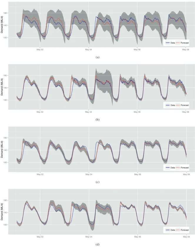
A sample of the forecasts for the hourly and sub-hourly models is presented in Fig. 2. Each plot shows the same data segment of 7 days along with the one-day-ahead forecasts and the uncertainty bands (95% confidence level) in grey at the corresponding resolution. The data segment starts Saturday and Monday is a bank holiday, hence the similarity of the demand during the three-day weekend. The consumption pattern changes from Tuesday through Friday, where sharper peaks appear in earlier hours of the day. The figure illustrates how the different models respond to the data characteristics.

The width of the uncertainty bands, illustrates the overall forecast error behaviour. Models with weekly seasonal periods (Figs. 2(b) and 2(d)) have narrower bands, i.e., higher overall forecast accuracies, than models with daily correlations (Figs. 2(d) and 2(c)). A complete picture of the performance of the models is presented in the error assessment section.

3.4. Model Performance Assessment

Each model type of Table 1 was able to produce a long time series of forecasts at its corresponding resolution. The RMSE (Eq. 2) was computed from the deviations of the forecasts with respect to the validation data series. In order to assess the performance, the NRMSE (Eq. 3) and the MAPE (Eq. 4) were also calculated. Table 3 summarises the results.

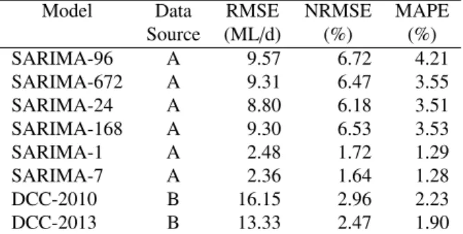
All three statistics follow similar trends for the six model types since the same validation data set was used. However, the MAPE is considered most meaningful in cross comparison because it normalises the errors at every measurement. The last two rows of Table 3 present the performance statistics of empirical production of the water utility in 2010 and 2013. The data corresponds to Source B and reﬂects the real performance in water production.

Table 3: Statistics for assessment of model performance and empirical production in DCC

Model Data RMSE NRMSE MAPE Source (ML/d) (%) (%) SARIMA-96 A 9.57 6.72 4.21 SARIMA-672 A 9.31 6.47 3.55 SARIMA-24 A 8.80 6.18 3.51 SARIMA-168 A 9.30 6.53 3.53 SARIMA-1 A 2.48 1.72 1.29 SARIMA-7 A 2.36 1.64 1.28 DCC-2010 B 16.15 2.96 2.23 DCC-2013 B 13.33 2.47 1.90

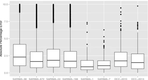
As a complement, Fig. 3 illustrates the distribution of the MAPE for each element of Table 3. The results show that the median percentage value for all models is below 2.5%. Models with higher resolution perform similarly, but the distribution of errors of models with weekly seasonal periods indicates a better performance. Such models are

(7)

100 140 180

May 02 May 04 May 06 May 08

Demand (ML/d) Data Forecast (a) 100 140 180

Demand (ML/d) Data Forecast (b) 100 140 180

Demand (ML/d) Data Forecast (c) 100 140 180

Demand (ML/d)

Data Forecast

(d)

Fig. 2: Sample of the demand forecasts by the models with sub-hourly and hourly resolutions. The grey bounds indicate the uncertainty (95% conﬁdence level). (a) SARIMA-96; (b) SARIMA-672; (c) SARIMA-24; (d) SARIMA-168.

(8)

recommended when the interest is in hourly demand forecasts. Clearly, the daily models have the smallest errors and both provide equivalent results, but SARIMA-7 is preferred due to a more compact distribution of errors.

0.0 2.5 5.0 7.5 10.0

SARIMA−96 SARIMA−672 SARIMA−24 SARIMA−168 SARIMA−1 SARIMA−7 DCC−2010 DCC−2013

Absolute P

ercentage Error

Fig. 3: Comparison of model and real performance

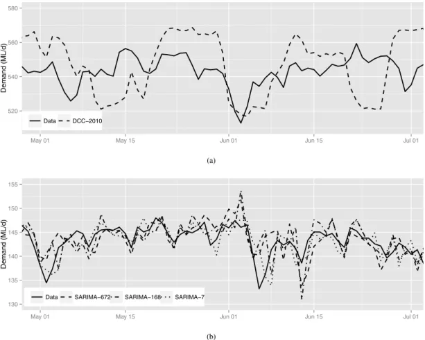
A graphical representation of the water production and the daily forecasts produced by the best performing models across the range of resolutions is presented ﬁn Fig. 4. It is clear that signiﬁcant deviations exist between the real consumption and production measurements. The MAPE of DCC production in 2010 is 2.23% which may be consid-ered an acceptable performance. The statistics above, however, show that time series models are able to improve the forecasts by reducing the MAPE to 1.28%. The error is thus reduced by 42.6% in magnitude and is also reduced in dispersion, meaning that large errors are less frequent.

4. Summary and Conclusions

The analysis presented provides insights on the time series models parameterisation and performance as well as on the effects of the temporal resolution when estimating daily water production. It was shown that the choice of model estimation window may have a considerable effect on the forecast accuracy. The minimal window lengths (7 d) required to fit a model are recommended for the 15-min and hourly models; larger windows (28 d) are preferred for the daily models; further enhancements may be obtained through an adaptive sizing of the training window. Among the hourly and sub-hourly models, the best performing is SARIMA-672, therefore it is recommended to forecast demands at the highest resolution. The SARIMA-168 is, however, preferred for hourly resolution because it is sufficiently accurate and requires only a fraction of the computational resources. For the purpose of daily production forecasting, the selected model is SARIMA-7 due to its remarkable accuracy. Future work to improve the models’ forecasting ability encompasses the introduction of weather covariates such as air temperature and rainfall, and a filtering method to reduce the estimation frequency in particular for the higher resolution models.

Acknowledgements

The authors would like to acknowledge the Dublin City Council for providing the water demand data used in this research.

(9)

520 540 560 580

May 01 May 15 Jun 01 Jun 15 Jul 01

Demand (ML/d) Data DCC−2010 (a) 130 135 140 145 150 155

May 01 May 15 Jun 01 Jun 15 Jul 01

Demand (ML/d)

Data SARIMA−672 SARIMA−168 SARIMA−7

(b)

Fig. 4: Plots of total system demand, water production, and forecasts at daily level. (a) Total system demand and production; (b) Demand data and daily forecasts.

References

[1] S. Wong, A model on municipal water demand: A case study of Northeastern Illinois, J. Water Resour. Plann. Manage. 48 (1972) 34–44. [2] J. Salas, V. Yevjevich, Stochastic structure of water use time series, Technical Report, Colorado State University, Fort Collins, CO, 1972. [3] H. Yamauchi, W. Huang, Alternative models for estimating the time series components of water consumption data, Water Resources Bulletin

13 (1977) 599–610.

[4] A. E. Cassuto, S. Ryan, Eﬀect of price on the residential demand for water within an agency, Jour. of the American Water Resour. Assoc. 15 (1979) 345–353.

[5] D. R. Maidment, S. P. Miaou, M. M. Crawford, Transfer function models of daily urban water use, Water Resources Research 21 (1985) 425–432.

[6] D. R. Maidment, S. P. Miaou, Daily water use in nine cities, Water Resources Research 22 (1986) 845–851.

[7] S. Zhou, T. McMahon, A. Walton, J. Lewis, Forecasting daily urban water demand: a case study of Melbourne, Journal of Hydrology 236 (2000) 153–164.

[8] J. Adamowski, H. F. Chan, A wavelet neural network conjunction model for groundwater level forecasting, Journal of Hydrology 407 (2011) 28–40.

[9] G. P. Zhang, An investigation of neural networks for linear time-series forecasting, Computers & Operations Research 28 (2001) 1183 – 1202. [10] A. Jain, L. E. Ormsbee, Short-term water demand forecast modeling techniques: Conventional methods versus AI, Jour. American Water

Works Assoc. 94 (2002) 64–72.

[11] J. Bougadis, K. Adamowski, R. Diduch, Short-term municipal water demand forecasting, Hydrological Processes 19 (2005) 137–148. [12] M. Ghiassi, D. Zimbra, H. Saidane, Urban water demand forecasting with a dynamic artiﬁcial neural network model, Jour. of Water Resour.

(10)

Plann. and Manage. 134 (2008) 138–146.

[13] J. Adamowski, H. F. Chan, S. O. Prasher, B. Ozga-Zielinski, A. Sliusarieva, Comparison of multiple linear and nonlinear regression, autore-gressive integrated moving average, artiﬁcial neural network, and wavelet artiﬁcial neural network methods for urban water demand forecasting in montreal, canada, Water Resources Research 48 (2012).

[14] M. K. Tiwari, J. Adamowski, Water demand forecasting and uncertainty assessment using ensemble wavelet-bootstrap-neural network models, Water Res. Research 49 (2013) 6486–6507.

[15] S. Srinivasulu, A. Jain, River ﬂow prediction using an integrated approach, J. Hydrol. Eng. 14 (2009) 75–83.

[16] A. Kant, P. K. Suman, B. K. Giri, M. K. Tiwari, C. Chatterjee, P. C. Nayak, S. Kumar, Comparison of multi-objective evolutionary neural network, adaptive neuro-fuzzy inference system and bootstrap-based neural network for ﬂood forecasting, Neural Computing and Applications 23 (2013) 231–246.

[17] D. R. Maidment, S.-P. Miaou, Daily water use in nine cities, Water Resources Research 22 (1986) 845–851. [18] R. Shumway, D. Stoﬀer, Time Series Analysis and Its Applications, Springer-Verlag GmbH, 2000.

[19] G. Box, G. Jenkins, G. Reinsel, Time Series Analysis: Forecasting and Control, Wiley Series in Probability and Statistics, Wiley, 2008. [20] G. Gardner, A. Harvey, G. Phillips, Algorithm AS154: An algorithm for exact maximum likelihood estimation of autoregressive-moving

average models by means of Kalman ﬁltering, Applied Statistics 29 (1980) 311–322.