Sparse estimation of high-dimensional time series models.

(1)

FACULTEIT ECONOMIE EN BEDRIJFSWETENSCHAPPEN

KU LEUVEN

Sparse estimation of high-dimensional time series models

Proefschrift Voorgedragen tot het Behalen van de Graad van Doctor in de Toegepaste Economische Wetenschappen door

Ines WILMS

(2)

(3)

Committee

Advisor:

Prof. Dr. Christophe Croux KU Leuven

Chair:

Prof. Dr. Robert Boute KU Leuven

Members:

Prof. Dr. Geert Dhaene KU Leuven

Prof. Dr. Sarah Gelper Technische Universiteit Eindhoven

Prof. Dr. Jeroen Rombouts ESSEC Business School

Prof. Dr. Martina Vandebroek KU Leuven

Daar de proefschriften in de reeks van de Faculteit Economie en Bedrijfswetenschappen het persoonlijk werk zijn van hun auteurs, zijn alleen

deze laatsten daarvoor verantwoordelijk.

(4)

(5)

Acknowledgments

This thesis concludes almost four years of intensive research. Several people have contributed to this work by giving professional and personal support.

First and foremost, I would like to express profound gratitude to my super-visor Prof. Christophe Croux. Thank you for sharing your expertise, for always believing in me, for providing a stimulating and motivating research environment, and for passing on your passion for conducting research. Conducting research and communicating it in an understandable way is not an easy task. Also here, thank you for being an excellent ‘teacher’. All chapters of this thesis have greatly im-proved by your suggestions and valuable feedback. It has been a privilege and pleasure to work with you and I hope we will continue our collaborations.

I would also like to thank all members of the doctoral committee: Prof. Geert Dhaene, Prof. Sarah Gelper, Prof. Jeroen Rombouts, and Prof. Martina Vande-broek. Thank you for the thorough reading of my thesis, and for all constructive comments during the doctoral seminars and preliminary defense. Your comments have led to a considerable improved quality of this text. Sarah, our collaborations on Chapter 1 and 3 have been very instructive, motivating and inspiring to me.

Furthermore, I am very grateful to the FWO (Fonds Wetenschappelijk On-derzoek Vlaanderen) for the financial support and to KU Leuven for providing me with the facilities to carry out this doctoral research. The statistical seminars organized by the LSTAT group have definitely broadened my knowledge.

I would also like to thank all my colleagues from ORSTAT, Heverlee and the ‘fourth floor’. Thank you for the pleasant working atmosphere. I really enjoyed our numerous joint activities. Special thanks to Viktoria for providing support from the beginning of my PhD until the end.

Tot slot wil ik nog graag mijn familie bedanken. Bedankt om er altijd voor mij te zijn, om me in alles aan te moedigen en te steunen.

Ines Wilms Leuven, April 2016.

(6)

(7)

Introduction

Nowadays, a large amount of data is available in nearly every area of science and business. Information is typically collected in data sets where the different variables are contained in the columns of the data set and the measurements on each variable are contained in the rows. Our interest mainly lies in settings where these measurements are collected over time. Such data sets are said to contain

time series in their columns. A time series should be treated differently from a regular variable to account for the time-dependency of its measurements. As an example, data sets in marketing containing weekly sales, price and promotional information on product categories (e.g. soft drinks) are typically available.

Moreover, given today’s data abundance, our interest lies inhigh-dimensional

data sets, as opposed tolow-dimensional data sets. High-dimensional time series data sets contain many short time series: a large number of time series (columns) is available relative to the number of time points (rows), hence, these data sets are ‘fat’. Low-dimensional time series data sets, in contrast, contain few long time series: a large number of time points (rows) is available relative to the number of time series (columns), hence, these data sets are ‘thin’. High-dimensional time series data sets are commonplace in today’s business practice since many firms collect information on a large number of variables, but discard data that are older than a few years. For instance, consider the goal in marketing to predict future sales volumes for a large number of product categories based on their past sales, price and promotional information. To obtain such predictions, an estimation method is needed.

The problem, however, is that traditional estimators are well suited for low-dimensional data sets, but not for high-low-dimensional data sets. On the one hand, these estimators suffer from very low estimation precision if the number of mea-surements (rows) is close to the number of variables (columns) in the data set. This leads towards inaccurate predictions. On the other hand, traditional

(8)

vi Introduction

tors are not even computable if the number of measurements (rows) in the data set is larger than the number of variables (columns). Then, no predictions can be made. Hence, there is a need for new estimation methods especially designed for these high-dimensional data sets.

In this thesis, we develop sparse estimation methods for high-dimensional data. Despite the data abundance, we do not expect each variable of these data sets to be equally informative. Sparse estimation methods rely on a simplicity assumption: we assume that only a relative small number of variables in our data set plays an important role. As such, sparse estimators retain the informative variables and remove the non-informative ones. In our marketing example, we do not expect that each variable will influence each category’s sales volume. Instead, we expect some variables to be unimportant in predicting these sales volumes, but we do not know which. Sparse estimators detect for each category the variables that are important for predicting its future sales volume, and it estimates the effect these variables have on its future sales volume. For the variables that are detected to be unimportant, their estimated effect is put to zero. This highly facilitates interpretation.

We develop sparse estimators for high-dimensional time series models in Chap-ters 1 to 4, and for Canonical Correlation Analysis (CCA) in ChapChap-ters 5 and 6. CCA is a multivariate statistical method that describes the associations be-tween two data sets. Our interest lies in settings where both data sets are high-dimensional. Throughout the thesis, the usefulness and relevance of the sparse estimators are discussed for a wide variety of application domains, ranging from marketing (Chapter 1), and economics (Chapter 3, 4), to biometrics (Chapter 2, 5, 6).

Chapter 1 is dedicated to the development of a sparse estimator for the high-dimensional Vector AutoRegressive (VAR) model. The VAR model is the pre-ferred model in econometrics to analyze the relationship between several time series. We focus on high-dimensional VAR models, models containing a large number of short time series. We show that more accurate estimation and pre-diction results are obtained with our sparse estimator compared to traditional estimators. We apply the sparse estimator of the VAR to a high-dimensional marketing data set where we predict sales volumes for a large number of product categories. The sparse estimator yields insightful results regarding which cat-egories are more influential (meaning that they are important drivers of other category’s sales), and which categories are more responsive (meaning that they react to changes in other categories).

(9)

Introduction vii

In Chapter 2, we develop a computational algorithm for sparse estimation of the general class of Multivariate Regression Models, of which the VAR model is a special case. In high-dimensional Multivariate Regression Models, a large number of response variables (not necessarily time series) is predicted using a large number of predictor variables. We illustrate the algorithm on a biometric data set. Biometrics is another field of science where high-dimensional data sets are commonplace. We consider a genomic data set that contains information on a large number of genes, but only a small number of measurements is available (often because of cost constraints).

Chapter 3 considers the popular time series concept of ‘Granger Causality’ in high-dimensions. A (set of) time series is said to Granger Cause another time series if the former has incremental, or additional, predictive power for the latter. We develop a new test procedure, called the ‘Granger Lasso test’, to test for Granger Causality in high-dimensional settings. We show that this test is more powerful than traditional tests in such settings. We use the proposed test to study the predictive power of economic sentiment indicators for future macro-economic developments. We find that forecast accuracy is improved by using only the most predictive sentiment indicators, obtained with the Granger Lasso test, rather than all indicators.

Chapter 4 considers another popular time series concept in high-dimensions, namely ‘Cointegration’. Cointegration analysis is used to estimate long-run equi-librium relations between several time series. The coefficients of these relations are called the ‘cointegrating vectors’. We provide a sparse estimator of the cointegrat-ing vectors. The proposed estimator is used for interest rate growth forecastcointegrat-ing and consumption growth forecasting. We show that it leads to important gains in forecast accuracy compared to traditional estimators.

In Chapter 5, we develop a sparse CCA method. The typical research field of interest is biometrics where one wants to study associations between one data set containing gene expression data and another containing comparative genomic hybridization data. Identifying associations between both is extremely important to increase our understanding of the development of diseases such as cancer. A sparse approach is often wanted to identify the most important variables for the association study. We illustrate the good performance of our proposed sparse CCA method compared to other sparse CCA alternatives by means of a simulation study and a biometric data example.

Finally, in Chapter 6, we address the frequent occurrence of outliers in high-dimensional data sets used for CCA. Outliers are observations with an atypical

(10)

viii Introduction

behavior, making it unlikely that they are generated by the model. In genomics, some patients can react very differently to treatments because of their individual-specific genetic structure. The possible presence of outlying observations should be taken into account and estimates should remain reliable, or ‘robust’, in their presence. In Chapter 6, we therefore robustify the sparse CCA method from Chapter 5. An additional advantage of the proposed robust sparse CCA method is that outliers can be identified. Knowledge of such atypical patients is extremely useful for geneticists.

The various chapters in this thesis can be found in

(i) S. Gelper, I. Wilms and C. Croux. Identifying demand effects in a large network of product categories. Journal of Retailing, 92(1), 25-39, 2016. (ii) I. Wilms and C. Croux. An algorithm for the multivariate group lasso with

covariance estimation. FEB Research Report KBI 1528, 2015.

(iii) I. Wilms, S. Gelper and C. Croux. The predictive power of the business and bank sentiment of firms: A high-dimensional Granger Causality approach.

European Journal of Operational Research,Accepted, 2016.

(iv) I. Wilms and C. Croux. Forecasting using sparse cointegration. Interna-tional Journal of Forecasting, Accepted, 2016.

(v) I. Wilms and C. Croux. Sparse canonical correlation analysis from a predic-tive point of view. Biometrical Journal, 57(5), 834-851, 2015.

(vi) I. Wilms and C. Croux. Robust sparse canonical correlation analysis. FEB Research Report KBI 1428, 2014.

(11)

Planning marketing mix strategies requires retailers to understand within-as well within-as cross-category demand effects. Most retailers carry products in a large variety of categories, leading to a high number of such demand effects to be estimated. At the same time, we do not expect cross-category ef-fects between all categories. This paper outlines a methodology to estimate a parsimonious product category network without prior constraints on its structure. To do so, sparse estimation of the Vector AutoRegressive Market Response Model is presented. We find that cross-category effects go beyond substitutes and complements, and that categories have asymmetric roles in the product category network. Destination categories are most influential for other product categories, while convenience and occasional categories are most responsive. Routine categories are moderately influential and moder-ately responsive.

1.1 Introduction

While within-category demand effects of the marketing mix have been studied extensively, cross-category effects are less well understood [Leeflang and Selva,

(16)

2 Sparse estimation of the VAR

2012]. Nevertheless, cross-category effects might be substantial. Some categories are complements, e.g. bacon and eggs studied by Niraj et al. [2008] or cake mix and cake frosting studied by Manchanda et al. [1999], while others are substitutes, e.g. frozen, refrigerated and shelf-stable juices [Wedel and Zhang, 2004]. But cross-effects also exist among categories that are not complements or substitutes for several reasons. First, as a result of brand extensions, brands are no longer limited to one category [Erdem, 1998, Kamkura and Kang, 2007, Ma et al., 2012]. So advertising and promotion of a brand within one category might spill over to own brand sales in other categories. Second, advertising and promotions generate more store traffic and therefore more sales in other categories [Bell et al., 1998]. And third, lower expenditures in one category alleviate the budget constraint such that consumers are able to spend more on other, seemingly unrelated, categories [Song and Chintagunta, 2007, Lee et al., 2013].

While cross-category effects might be substantial for these reasons, we do not expect that each category’s marketing mix variables influence each and every other category. Instead, we expect some cross-category effects to be zero – or very close to zero – but we can not a priori exclude them. Therefore, we use an exploratory modeling approach for parsimonious estimation of a product category network. The network allows us to easily identify categories that are influential for or responsive to changes in other categories. Building on a widely used category typology of destination, routine, occasional and convenience categories [Blattberg et al., 1995, Briesch et al., 2013], we find that destination categories are most influential, convenience and occasional categories most responsive, and routine categories moderately influential and moderately responsive.

In order to estimate the cross-category network, this paper presents sparse estimation of the Vector AutoRegressive (VAR) model. The estimation issparse

in the sense that some of the within-and cross-category effects in the model can be estimated as exactly zero. Initiated by the work of Baghestani [1991] and Dekimpe and Hanssens [1995], the VAR Market Response Model has become a standard, flexible tool to measure own- and cross-effects of marketing actions in a competitive environment. The main drawback of the VAR model is the risk of overparametrization because the number of parameters increases quadratically with the number of included categories. Earlier studies using the VAR model, like e.g. Nijs et al. (2001; 2007); Pauwels et al. [2002]; Srinivasan et al. (2000; 2004); Steenkamp et al. [2005], were often limited by this overparametrization problem. To overcome this problem, previous research on cross-category effects has limited its attention to a small number of categories by studying substitutes or

(17)

comple-1.2. Cross-Category Management 3

ments [Kamkura and Kang, 2007, Song and Chintagunta, 2007, Leeflang et al., 2008, Bandyopadhyay, 2009, Ma et al., 2012]. We present an estimation tech-nique for cross-category effects in much larger product category networks. The technique allows many parameters to be estimated even with short observation periods. Short observation periods are commonplace in marketing practice since many firms discard data that are older than one year [Lodish and Mela, 2007].

This paper contributes to the extant retail literature in a number of important ways. (1) Previous cross-category literature largely limits attention to categories that are directly related through substitution, complementarity or brand exten-sions. We provide evidence that cross-category effects go beyond such directly related categories. (2) We introduce the concepts of influence and responsiveness of a product category and position different category types (destination, routine, occasional and convenience) according to these dimensions. (3) To identify the cross-category effects, we estimate a large VAR model using an extension of the lasso approach of Tibshirani [1996].

The remainder of this article is organized as follows. Section 1.2 positions this paper in the cross-category management literature and describes the conceptual framework that positions category types according to their influence and respon-siveness. Section 1.3 discusses the methodology. We describe the sparse estimator of the VAR model, discuss how to construct impulse response functions and com-pare the sparse estimation technique with two Bayesian estimators. In Section 1.4, a simulation study shows the excellent performance of the proposed methodology in terms of estimation reliability and prediction accuracy. Section 1.5 presents our data and model, Section 1.6 our findings on cross-category demand effects. We first identify which categories are most influential and which are most responsive to changes in other categories. Then, we identify the main cross-category effects based on estimated cross-price, promotion and sales elasticities.

1.2 Cross-Category Management

The importance of category management for retailers is widely acknowledged, both as a marketing tool for category performance [Fader and Lodish, 1990, Ba-suroy et al., 2001, Dhar et al., 2001] and as an operational tool for planning and logistics [Rajagopalan and Xia, 2012]. Successful category management re-quires retailers to understand cross-category effects of prices, promotions and sales. Among these, the cross-category effects of prices on sales – which define substitutes and complements – are the most extensively studied [Song and

(18)

Chin-4 Sparse estimation of the VAR

tagunta, 2006, Bandyopadhyay, 2009, Leeflang and Selva, 2012, Sinistyn, 2012]. Cross-category effects of promotions, e.g. feature and display promotions, on sales result from many brands being active in multiple categories [Erdem and Sun, 2002]. Brand associations carry over to products of the same brand in other cat-egories, e.g. through umbrella branding [Erdem, 1998] or horizontal product line extensions [Aaker and Keller, 1990]. Less well understood than the effects of prices and promotions, are the effects of sales in one category on sales in other categories. Such effects might exist because categories are related based on affinity in con-sumption [Shankar and Kannan, 2014], because products from various categories are placed close to each other in the shelves [Bezawada et al., 2009, Shankar and Kannan, 2014], or because of the budget constraint [Du and Kamakura, 2008]. If consumers spend more in a certain category they might, all else equal, spend less in other categories simply because they hit their budget constraint. As a result, cross-category effects might exist between seemingly unrelated categories.

When studying these cross-category effects of price, promotion and sales on sales, several asymmetries might arise. A first asymmetry concerns within- versus cross-category effects. We expect within-category effects to be more prevalent and larger in size than cross-category effects (e.g. Song and Chintagunta, 2006; Bezawada et al., 2009). A second asymmetry concerns category influence ver-sus category responsiveness. Influential categories are important drivers of other category’s sales, while sales of responsive categories react to changes in other cat-egories. To identify which categories are more influential or more responsive, we build on a widely used typology of categories described in Blattberg et al. [1995]. Blattberg et al. [1995] define 4 category types from the consumer perspective: destination, routine, occasional and convenience. Destination categories contain goods that consumers plan to buy before they go on a shopping trip, such as soft drinks. Briesch et al. [2013] show that destination categories are generally categories in which consumers spend a lot of their budget. Retailers typically use a price aggressive promotion strategy and high promotion intensity for these destination categories with the goal of increasing store traffic. Because consumers shop to buy products in the destination categories, destination categories are likely to influence sales in other categories. However, since consumers already plan to buy in the destination categories before entering the store, destination category sales will not be highly responsive [Shankar and Kannan, 2014].

About 55% to 60% of categories are routine categories [Pradhan, 2009]. Rou-tine categories are regularly and rouRou-tinely purchased, such as juices and biscuits. Retailers typically use a consistent pricing strategy and average level of

(19)

promo-1.3. Sparse Vector Auto-Regressive Modeling 5

tion intensity. Because purchases in routine categories can more easily be delayed than purchases in destination categories, we expect routine categories to be more responsive. But, since purchases in routine categories altogether still account for a large portion of the budget, they are also likely to influence sales in other categories.

Occasional categories follow a seasonal pattern or are purchased infrequently. These categories comprise a small proportion of retail expenditures while they contain typically more expensive items, like oatmeal. We therefore expect occa-sional categories to be less influential and more responsive than destination or routine categories.

Finally, convenience categories are categories that consumers find convenient to pick up during their one-stop shopping trip, like ready-to-eat-meals. These purchase decisions are typically made in the store. Since convenience categories are geared towards consumer convenience and filling impulse needs, we expect them to be highly responsive.

1.3 Sparse Vector Auto-Regressive Modeling

1.3.1 Motivation

The aim of this paper is to identify cross-category demand effects in a large prod-uct category network. To this end, we use the Vector AutoRegressive (VAR) model. The VAR is ideal for measuring within- and cross-category effects of mar-keting actions since it accounts for both inertia in marmar-keting spending and perfor-mance feedback effects by treating marketing variables as endogenous [Dekimpe and Hanssens, 1995]. Other studies on cross-category effects, like e.g. Wedel and Zhang [2004] use a demand model with exogenous prices, or a simultaneous equa-tions model without lagged effects like Shankar and Kannan [2014]. However, managers may set marketing instruments strategically in response to market per-formance and market response expectations. Not accounting for time inertia or feedback effects limits our understanding of how the market functions and mis-leads managerial insights and prediction.

Identifying cross-category demand effects using VAR analysis remains chal-lenging because the sheer number of such effects makes them hard to estimate. The number of parameters to be estimated in the VAR rapidly explodes, making standard estimation inaccurate. This undermines the ability to identify important relationships in the data. To overcome an explosion of the number of parameters

(20)

in the VAR, marketing researchers have used pre-estimation dimension reduction techniques, i.e. they first impose restrictions on the model and then estimate the reduced model. Four such common techniques are (i) treating marketing variables as exogenous (e.g. Nijs et al., 2001; Pauwels et al., 2002 and Nijs et al., 2007), (ii) estimating submodels rather than a full model (e.g. Srinivasan et al., 2000; Srinivasan et al., 2004), (iii) aggregating or pooling over, for instance, stores or competitors (e.g. Horvath et al., 2005; Slotegraaf and Pauwels, 2008), and (iv) applying Least Squares to a restricted model (e.g. Dekimpe and Hanssens, 1995, Dekimpe et al., 1999; Nijs et al., 2007). Most researchers applying pre-estimation dimension reduction techniques recognize that they do so because of the practical limitations of standard estimation techniques rather than for theoretical reasons (e.g. Srinivasan et al., 2004 and Bandyopadhyay, 2009).

To address the overparametrization of the VAR, we use sparse estimation. Sparsity means that some of the within- and cross-category effects in the VAR are estimated as exactly zero. As argued in the previous section, from a substantive perspective, we cannot exclude cross-category effects before estimation because cross-category effects might occur between seemingly unrelated categories. From a methodological perspective, sparse estimation is a powerful solution to handle the overparametrization of the VAR. In our cross-category model, we endogenously model sales, promotion and prices of 17 product categories. Hence, already in a VAR model with one lag, as much as (3×17)×(3×17) = 2601 within- and cross-category effects need to be estimated. Since the sparse estimation procedure puts some of these effects to zero, a more parsimonious model is obtained. Results are easier to interpret and, therefore, the sparse estimation procedure provides actionable insights to managers.

1.3.2 Extending the Lasso to the VAR model

In situations where the number of parameters to estimate is large relative to the sample size, the Lasso proposed by Tibshirani [1996] provides a solution within the multiple regression model. The Lasso minimizes the least squares criterion penalized for the sum of the absolute values of the regression parameters. This penalization forces some of the estimated regression coefficients to be exactly zero, which results in selection of the pertinent variables in the model. The Lasso method is well established [B¨uhlmann and van de Geer, 2011, Chatterjee and Lahiri, 2011] and shows good performance in various applied fields [Wu et al., 2009, Fan et al., 2011].

(21)

1.3. Sparse Vector Auto-Regressive Modeling 7

The Lasso technique can not be directly applied to the VAR model because the VAR model differs from a multiple regression model in two important aspects. First, a VAR model contains several equations, corresponding to a multivariate regression model. Correlations between the error terms of the different equations need to be taken into account. Second, a VAR model is dynamic, containing lagged versions of the same time series as right-hand side variables of the regression equation. Both aspects of VAR models make it necessary to extend the lasso to the VAR context, what the sparse estimator in this paper does.

It builds further on a sparse estimator of the multivariate regression model [Rothman et al., 2010], and the groupwise lasso for categorical variables [Yuan and Lin, 2006, Meier et al., 2008]. The estimator is consistent for the unknown model parameters, see Meier et al. [2008] and Friedman et al. [2008].

1.3.3 Model Specification

Sales, price and promotion are measured for several categories over a certain time period. We collect all these time series in a multivariate time series yt with q

components. In our cross-category demand effects study,ytcontains sales, price

and promotion for 17 product categories, henceq= 3×17 = 51. The VAR Market Response Model is given by

yt=B1yt−1+B2yt−2+. . .+Bpyt−p+et, (1.1)

where pis the lag length. The autoregressive parameters B1 to Bp are (q×q)

matrices, which capture both within- and cross-category effects. The elements of these matrices measure the effect of sales, price and promotion in one category on the sales, price and promotion in other categories (including its own). The error termetis assumed to follow a Nq(0,Σ) distribution. We assume, without

loss of generality, that all time series are mean centered such that no intercept is included.

If the number of components q in the multivariate time series is large, the number of unknown elements in the sequence of matricesB1, . . . ,Bp explodes to

pq2_{, and accurate estimation by standard methods is no longer possible. Sparse} estimation, with many elements of the matrices B1, . . . ,Bp estimated as zero,

brings an outcome: it will not only provide estimates with smaller mean squared error, but also substantially improve model interpretability. The method we pro-pose does not require the researcher to prespecify which entries in theBjmatrices

(22)

si-8 Sparse estimation of the VAR

multaneously performed. This is particularly of interest in situations where there is no a priori information on which time series is driving which.

The instantaneous correlations in model (1.1) are captured in the error covari-ance matrixΣ. If the dimensionqis large relative to the number of observations, estimation ofΣbecomes problematic. The estimated covariance matrix risks get-ting singular, i.e. its inverse does not exist. Hence, we also induce sparsity in the estimation of the inverse error covariance matrix Ω=Σ−1_{. The elements of} _Ω have a natural interpretation as partial correlations between the error components of the q equations in model (1.1). If the ij-th element of the inverse covariance matrix is zero this means that, conditional on the other error terms, there is no correlation between the error terms of equationsiandj.

1.3.4 Penalized Likelihood Estimation

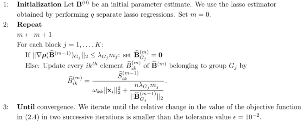
This section defines the sparse estimation procedure for the VAR model. The Sparse VAR estimator is defined by minimizing a measure of goodness-of-fit to the data combined with apenaltyfor the magnitude of the model parameters. It is convenient to first recast model (1.1) in stacked form as

y=Xβ+e, (1.2)

wherey is a vector of lengthnqcontaining the stacked values of the time series. If the multivariate time series has lengthT, thenn=T−pis the number of time points for which all current and lagged observations are available. The vectorβ

contains the stacked vectorized matricesB1, . . . ,Bp, andethe vector of stacked

error terms. The matrixX=Iq⊗X0, with X0= (Y1, . . . ,Yp), is of dimension

(nq×pq2_{). Here}_Y

j is an (n×q) matrix, containing the values of the q series

at lagj in its columns, for 1≤j ≤p, withpthe maximum lag. The symbol ⊗

stands for the Kronecker product.

The sparse estimator of the autoregressive parameters β and the inverse co-variance matrixΩ=Σ−1_{are obtained by minimizing the negative log likelihood} with a groupwise penalization on the β and a penalization on the off-diagonal elements ofΩ: (βb,Ω) = argminb (β,Ω) 1 n(y−Xβ) T e Ω(y−Xβ)−log|Ω|+λ1 G X g=1 ||βg||+λ2 X k6=k0 |Ωkk0|, (1.3) where||u||= (Pn i=1u 2

i)1/2 is the Euclidean norm and Ωe =Ω⊗In. By

(23)

1.3. Sparse Vector Auto-Regressive Modeling 9

terms into account. The vector βg in (1.3) is a subvector ofβ, containing the

regression coefficients for the lagged values of the same time series in one of the

qequations in model (1.1). The coefficients of the lagged values of the same time series form a group. The total number of groups is G=q2 because there are q

groups within each of theqequations. The penalty on the regression coefficients enforces that eitherall elements of the groupβbg are zero ornone. As a result, we

take the dynamic nature of the VAR model into account since the estimatedBj

matrices, forj= 1, . . . , p, have their zero elements in exactly the same cells. The penalization on the off-diagonal elements of Ω induces sparsity in the estimate

b

Ω. Finally, the scalarsλ1 andλ2 control the degree of sparsity of the regression estimator and the inverse covariance matrix estimator, respectively. The larger these values, the more sparsity is imposed. Details on the algorithm to perform penalized likelihood estimation and the selection of the sparsity parameters λ1 andλ2can be found in Appendix 1.8.

Our approach is similar to Hsu et al. [2008] who use the Lasso within a VAR context. However, they do not account for the group-structure in the VAR model, nor do they impose sparsity on the error covariance matrix. Davis et al. [2015] propose another sparse estimation procedure for the VAR. They infer the sparsity structure of the autoregressive parameters from an estimate of the partial spectral coherence using a two-step procedure. Since variable selection is performed prior to model estimation, the resulting estimator suffers from pre-testing bias. More-over, the number of parameters might still approach the sample size, leading to unstable estimation or even making estimation infeasible if the number of param-eters still exceeds the sample size. Sparse estimation in economics is a growing field, see Fan et al. [2011] and references therein for an overview.

1.3.5 Alternative: Bayesian Estimators

An alternative to the sparse estimation technique is to impose prior information in a Bayesian setting. Bayesian regularization techniques have been proposed for the VAR model in Litterman [1980] and are used in various applied fields such as macroeconomics [Gefang, 2014, Banbura et al., 2010], finance [Carriero et al., 2012] and marketing [Lenk and Orme, 2009, Horvath and Fok, 2013, Bandyopad-hyay, 2009]. They are also applicable to a situation like ours where there are many parameters to be estimated with a limited observation period, and are thus a good benchmark. However, these methods are not sparse, they do not perform variable selection simultaneously with model estimation. The following two paragraphs

(24)

elaborate on two Bayesian estimators which serve as non-sparse alternatives.

Minnesota Prior. The original Minnesota prior only specifies a prior distribu-tion for the regression parameters of the VAR model. The error covariance matrix Σ is assumed to be diagonal, and estimated by ˆΣii = ˆσi2 with ˆσ2i the standard

OLS estimate of the error variance in an AR(p) model for theith_{time series [Koop}

and Korobilis, 2009]. The prior distribution of the regression parameters is taken to be multivariate normal:

β∼N(β_M,V_M). (1.4)

For the prior mean, the common choice isβ

M =0Kq for stationary series. The

prior covariance matrixV_M is diagonal. The posterior distribution is again mul-tivariate normal. Full technical details can be found in Koop and Korobilis [2009]. The main advantage of the Minnesota prior is its ease of implementation, since posterior inference only involves the multivariate normal distribution. How-ever, imposing the Minnesota prior only ensures that the parameter estimates are

shrunkentowards zero, while the Sparse VAR ensures that some parameters will be estimated asexactly zero.

Normal Inverted Wishart Prior. The Minnesota prior takes the error covari-ance matrixΣ as fixed and diagonal and, hence, not as an unknown parameter. To overcome this problem, Banbura et al. [2010] impose an inverse Wishart prior on theΣ matrix. More precisely,

β|Σ∼N(β

N IW,Σ⊗Ω0) and Σ∼iW(S0, ν0), (1.5)

where β

N IW,Ω0,S0 and ν0 are hyperparameters. Under this normal inverted

Wishart prior (labeled in the remainder of this paper as ‘NIW’), the posterior for

β, conditional onΣis normal, and the posterior forΣis again inverted Wishart. Full technical details can be found in Banbura et al. [2010].

1.3.6 Impulse Response Functions

Impulse response functions (IRFs) are extensively used to assess the dynamic effect of external shocks to the system such as changes in the marketing mix. An IRF pictures how a change to a certain variable at moment t impacts the value of any other time series at timet+k, accounting for interrelations with all other variables. The magnitude of the effect is plotted as a function of k. An extensive discussion on the interpretation of the IRF in marketing modeling can

(25)

1.4. Estimation and prediction performance 11

be found in Dekimpe and Hanssens [1995]. We use IRFs to gain insight in the dynamics of within and cross-category sales, promotion and price effects on each of the 17 product category sales. The IRFs are easily computed as a function of the Sparse VAR estimator (see Hamilton, 1991). Since we want to account for correlated error terms, we use generalized IRFs [Pesaran and Shin, 1998, Dekimpe and Hanssens, 1999].

To obtain confidence bounds for the generalized IRFs estimated by Sparse VAR, we use a residual parametric bootstrap procedure [Chatterjee and Lahiri, 2011]. We generateNb= 1000 time series of lengthT from the VAR model (1.2).

The invertible estimate ofΣ delivered by the Sparse VAR estimation procedure is needed to draw random numbers for theNq(0,Σ) error distribution. For each

of these Nb multiple time series, the estimates of the regression parameters are

computed. We compute the covariance matrix of theNbbootstrap replicates. For

each of theNbgenerated series impulse response functions are computed; the 90%

confidence bounds are then obtained by taking the 5% and 95% percentiles.

1.4 Estimation and prediction performance

We conduct a simulation study to compare the proposed Sparse VAR with Bayesian methods using the Minnesota and NIW prior. As benchmarks, we include the classical Least Squares (LS) estimator and two restricted versions of LS which are often used in practice. In the 1-step Restricted LS [Dekimpe and Hanssens, 1995, Dekimpe et al., 1999], we estimate the model with classical LS, delete all variables with|t-statistic| ≤1, and re-estimate the model with the remaining vari-ables. We also consider an iterative Restricted LS method described in L¨utkepohl and Kratzig [2004] where we fit the full model using LS and sequentially eliminate the variables leading to the largest reduction of BIC until no further improvement is possible, of which a close variant was used by Nijs et al. [2007].

We simulate from a VAR model withq= 30 dimensions andp= 2 lags. Each time series has an own auto-regressive structure and we include system dynamics among the different series. The first series leads series 2 to 15, while the 16th series leads time series 17 to 30. Specifically, the data generating processes are given by yt= " B1 0 0 B1 # yt−1+ " B2 0 0 B2 # yt−2+et,

(26)

12 Sparse estimation of the VAR with B1= " 0.41×1 01×14 0.414×1 0.4·I14 # and B2= " 0.21×1 01×14 0.214×1 0.2·I14 # .

In total, there arepq2_{= 1800 regression parameters to be estimated with 116} true parameter values different from zero. The 30-dimensional error term et is

drawn from a multivariate normal with mean zero and covariance matrix Σ = 0.1I30. We generateNs= 1000 multivariate time series of length 80 according to

the above simulation scheme.

1.4.1 Performance measures

We evaluate the different estimators in terms of (i) estimation accuracy, (ii) spar-sity recognition performance, and (iii) forecast performance.

To evaluate estimation accuracy, we compute the mean absolute estimation error (MAEE), averaged over the simulation runs and over the 1800 parameters

MAEE = 1 Ns 1 pq2 Ns X s=1 p X j=1 q X k,l=1 |ˆbsklj−bklj|,

where ˆbs_klj is the estimate ofbklj, theklthelement of the matrixBjcorresponding

to lagj, for thesth_{simulation run.}

Concerning sparsity recognition, we compute the true positive rate and true negative rate TPR = 1 Ns Ns X s=1 #{(k, l, j) : ˆbs klj 6= 0and bklj 6= 0} #{(k, l, j) : bklj 6= 0} TNR = 1 Ns Ns X s=1 #{(k, l, j) : ˆbs klj= 0 and bklj = 0} #{(k, l, j) : bklj = 0} .

The true positive rate (TPR) gives an indication on the number of true relevant regression parameters detected by the estimation procedure. The true negative rate (TNR) measures the hit rate of detecting a true zero regression parameter. Both should be as large as possible.

Finally, we conduct an out-of-sample rolling window forecasting exercise. Us-ing the same simulation design as before, we generate multivariate time series of length T = 90, and use a rolling window of length S = 80. For all estimation methods, 1-step-ahead forecasts are computed for t = S, . . . , T −1. Next, we

(27)

1.4. Estimation and prediction performance 13

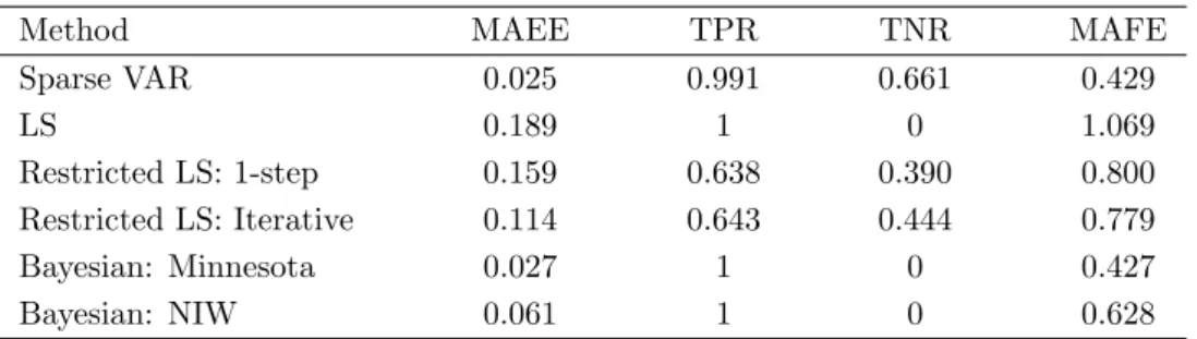
Table 1.1: Mean Absolute Estimation Error (MAEE), True Positive Rate (TPR), True Negative Rate (TNR) and Mean Absolute Forecast Error (MAFE), averaged over 1000 simulation runs, are reported for every method.

Method MAEE TPR TNR MAFE

Sparse VAR 0.025 0.991 0.661 0.429 LS 0.189 1 0 1.069 Restricted LS: 1-step 0.159 0.638 0.390 0.800 Restricted LS: Iterative 0.114 0.643 0.444 0.779 Bayesian: Minnesota 0.027 1 0 0.427 Bayesian: NIW 0.061 1 0 0.628

compute the mean absolute forecast error (MAFE), averaged over all time series and across time

MAFE = 1 T−S 1 q T−1 X t=S q X i=1 |yˆ(_t₊₁i) −y(_t₊₁i) |,

wherey_t(₊₁i) is the value of theith_{time series at time} _t_{+ 1.}

1.4.2 Results

Table 1.1 presents the performance measures of the Sparse VAR, the Bayesian and benchmark methods. The Sparse VAR estimator performs best in terms of estimation accuracy. It attains the lowest value of the MAEE (0.025). A paired

t-test confirms that the Sparse VAR significantly outperforms the other methods (allp-values<0.01).

Sparsity recognition performance is evaluated using the true positive rate and the true negative rate, reported in Table 1.1. For the LS and Bayesian estimators, all parameters are estimated as non-zero, resulting in a perfect true positive rate and zero true negative rate. Among the variable selection methods, the Sparse VAR performs best. Sparse VAR achieves a value of the true positive rate of 0.99; 0.66 for the true negative rate.

Finally, we evaluate the forecast performance of the different estimators by the Mean Absolute Forecast Error in Table 1.1. The Sparse VAR and the Bayesian estimator with Minnesota prior achieve the best forecast performance. A Diebold-Mariano test [Diebold and Diebold-Mariano, 1995] confirms that these two methods

(28)

per-14 Sparse estimation of the VAR

form significantly better than the others (p-values<0.01). There is no significant difference in forecast performance between Sparse VAR and the Bayesian estima-tor with Minnesota prior.

1.4.3 Robustness checks

Alternative penalty function. We investigate the robustness of Sparse VAR to the choice of the penalty function. We replace the grouplasso penalty on the regression coefficients with the elastic net penalty [Zou and Hastie, 2005]. Elastic net is a regularized regression method that linearly combines theL1 and L2 penalties of respectively lasso and ridge regression. Like the grouplasso, elastic net produces a sparse estimate of the regression coefficients. All other steps of the methodology remain unchanged. We find that the grouplasso penalty performs slightly better than the elastic net penalty in terms of estimation accuracy, sparsity recognition and prediction performance.

Sensitivity to the order of the VAR.We estimate the model with Sparse VAR for different values ofpand evaluate the performance. As expected, Sparse VAR attains the best estimation accuracy for the true valuep = 2. The results are, however, very robust to the choice of the order of the VAR. Selectingptoo low is slightly worse than selectingptoo high.

Sensitivity to the sparsity parameters. The sparsity parameters are selected according to the BIC and this selection is an integral part of the estimation procedure. The results are not sensitive to the value of λ2, which controls the sparsity ofΩ. The results are more sensitive to the choice ofb λ1, since it directly influences the sparsity of the autoregressive parameters. It turns out that Sparse VAR still outperforms the other estimators for a large range ofλ1 values.

1.5 Data and Model

We use the sparse estimation technique for large VARs described in Section 1.3 to identify cross-category demand effects across 17 categories in the Dominick’s Finer Foods database. This database is a well-established source of weekly scanner data from a large Midwestern supermarket chain, Dominick’s Finer Foods (e.g. Kamkura and Kang, 2007, Pauwels, 2007). We first describe the data and model in more detail, and then report on the insights the Sparse VAR generates in the next section.

(29)

1.5. Data and Model 15

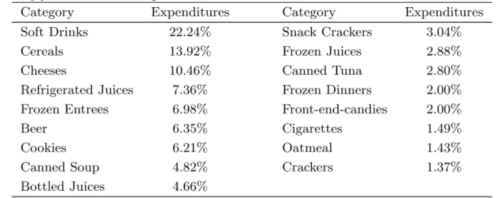
Table 1.2: Description of the 17 categories from Dominick’s Finer Foods database that are analyzed in this paper. For each category, we report the propor-tion of food and drink expenditures.

Category Expenditures Category Expenditures

Soft Drinks 22.24% Snack Crackers 3.04%

Cereals 13.92% Frozen Juices 2.88%

Cheeses 10.46% Canned Tuna 2.80%

Refrigerated Juices 7.36% Frozen Dinners 2.00%

Frozen Entrees 6.98% Front-end-candies 2.00%

Beer 6.35% Cigarettes 1.49%

Cookies 6.21% Oatmeal 1.43%

Canned Soup 4.82% Crackers 1.37%

Bottled Juices 4.66%

We use all 17 product categories in the Dominick’s Finer Foods database containing food and drink items, a much broader selection of categories than previous studies on cross-category demand effects have considered. A description of each product category can be found in Table 1.2. For 15 stores, we obtain weekly sales, pricing and promotional feature and display data for the 17 product categories.

Sales. Category sales volumes for the 17 categories, measured in dollars per week. Promotion. The promotional data include the percentage of SKUs of each cate-gory that are promoted (feature and display) in a given week, following Srinivasan et al. [2004].

Prices. To aggregate pricing data from the SKU level to the product category level, we follow Srinivasan et al. [2004] and Pauwels et al. [2002] in using SKU market shares as weights. Prices are not deflated because there is strong evidence that people are sensitive to nominal rather than real price changes [Shafir et al., 1997] over short time periods.

We use data from January 1993 to July 1994, 77 weeks in total. We neither use data before 1993 since they contain missing observations, nor observations after 1994 since Srinivasan et al. [2004] pointed out that manufacturers made extensive use of ‘pay-for-performance’ price promotions as of 1994, which are not fully reflected in the Dominick’s database. This data range is short relative to the dimension of the VAR, which calls for a regularization approach such as the Sparse VAR. For all stores, we collect data on sales, promotion and pricing for all

(30)

Table 1.3: Description of the 15 data sets. Each data set contains multivariate time series for sales (Yt), promotion (Mt) and prices (Pt).

Store Number of Dimension

Time Points Yt Mt Pt Total

Store 1-15 77 17 16 17 50

17 categories. Only for cigarettes, no promotion variable is included in the VAR since none of the SKUs in that category were promoted during the observation period.

We estimate a separate VAR model for each store, which allows to evaluate the robustness of the findings. The multivariate time series entering the VAR model are the log-differenced sales (Yt), differenced promotion (Mt), and log-differenced

prices (Pt).1 The dimensions of the time series are represented in Table 1.3. We

use the Vector Autoregressive model, with endogenous promotion and prices,

   Yt Mt Pt   =B0+B1    Yt−1 Mt−1 Pt−1   +. . .+Bp    Yt−p Mt−p Pt−p   +et. (1.6)

Averaged across stores, the selected value of pis two for the Sparse VAR. Also for the Bayesian estimators, the lag order of the VAR is selected using the BIC criterion, which is one for the majority of the stores.

1.6 Empirical Results

We focus on the effects of prices, promotions and sales in category A on the sales (or demand) in category B, where A and B belong to the product category net-work. We first study the direct effects. For instance, there is no direct effect of price of A on sales of B if the corresponding estimated regression coefficients are equal to zero at all lags. Then we turn to the complete chain of direct and indirect effects using Impulse Response Functions. For instance, price in category A indirectly influences sales in category B when the price of category A influences the price, promotion or sales in a certain other category C which, in turn, influ-ences the sales of category B. Since we work in a time series setting, both direct

1 _{Following standard practice, we first test for stationarity. A stationarity test of all individual}

time series using the Augmented Dickey-Fuller test indicates that most time series in levels are integrated of order 1.

(31)

1.6. Empirical Results 17

Table 1.4: Proportion of nonzero within and cross-category effects of price, pro-motion and sales on sales, averaged across 15 stores and 17 product categories.

Price Promotion Sales

Within-category 34% 30% 96%

Cross-category 19% 21% 21%

and indirect effects are dynamic in the sense that the effect occurs with a certain delay.

1.6.1 A network of product categories

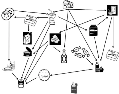
We analyze cross-category demand effects as a network of interlinked product categories of which prices, promotions and sales in one category have an effect on sales in other categories. Recently, network perspectives have been increasingly used by marketing researchers to model, for example, the network value of a product in a product network [Oestreicher-Singer et al., 2013] or to investigate the flow of influence in a social network [Zubcsek and Sarvary, 2011]. In our case, the 17 product categories are the nodes of the network. We estimate the Sparse VAR for 15 stores separately. If the Sparse VAR estimation results indicate, by giving a non-zero estimate, that prices in one category have a direct influence on sales in another category in the majority of the 15 stores, a directed edge is drawn between them. The resulting directed network is plotted in Figure 1.1. Similarly, Figures 1.2 and 1.3 present cross-category effects of respectively promotion and sales on sales. If promotion or sales in one category directly influence sales in another category, respectively, this is indicated by a directed edge.

A first important finding is that the cross-category networks are sparse – not each category influences each and every other category. While the sparse VAR estimation favors zero-effects, it does not enforce them. Here, as many as 78% of all estimated effects are zero-effects. Table 1.4 summarizes the prevalence of within-and cross-category effects. As expected, within-category effects are more common than cross-category effects. For all categories, past values of the own category’s sales are selected for almost all stores. Cross-category effects of price on sales (19%), promotion on sales (21%) and sales on sales (21%) are about equally prevalent.

Next, we focus on category influence and responsiveness in the cross-category network, measured by the number of edges originating from and pointing to a

(32)

Figure 1.1: Cross-category effect network of prices on sales: a directed edge is drawn from one category to another if its price influences sales in the other category for the majority of stores.

category respectively. As discussed in Section 1.2, destination categories are ex-pected to be more influential, while convenience categories are exex-pected to be more responsive. We discuss which types of categories we find to be most influen-tial and/or responsive in the cross-category networks of prices on sales, promotion on sales, and sales on sales.

The most influential categories in the cross-category network of prices on sales are destination categories such as Soft Drinks and Cheeses (cfr. each four outgoing edges in Figure 1.1). This is consistent with our expectations, as Soft Drinks is known to be a destination category [Briesch et al., 2013, Shankar and Kannan, 2014, Blattberg et al., 1995]. Soft Drinks is ranked first and Cheeses third in terms of food and drink expenditures (see Table 1.2) and are both heavily pro-moted by retailers. A price change in either of these categories thus strongly

(33)

Figure 1.2: Cross-category effect network of promotions on sales: a directed edge is drawn from one category to another if its promotion influences sales in the other category for the majority of stores.

influences the budget constraint, which in turn influences purchase decisions in other categories. In the cross-category network of promotions on sales, Cereals is the most influential category (cfr. five outgoing edges in Figure 1.2). Briesch et al. [2013] identified Cereals as highly ranked among the destination categories. This is not surprising as cereals are part of daily consumption patterns and are ranked second in terms of food and drink expenditures. In the cross-category effects network of sales on sales in Figure 1.3, we identify again Cheeses as the most influential category.

We find convenience categories to be highly responsive to changes in other categories. The most prominent price effects are observed for Canned Soup (cfr. five incoming edges in Figure 1.1); the most prominent promotion effects for Frozen Dinners, Crackers and Canned Soup (cfr. each three incoming edges in

(34)

Figure 1.3: Cross-category effect network of sales on sales: a directed edge is drawn from one category to another if its sales influences sales in the other cate-gory for the majority of stores.

Figure 1.2); and the most prominent sales effects for Oatmeal and Crackers (cfr. each four incoming edges in Figure 1.3). These categories are typically bought out of convenience, such as Frozen Dinners and Canned Soup; or bought on occasion, such as Oatmeal and Crackers, counting for a very small percentage of food and drink expenditures (see Table 1.2).

Routine categories such as Bottled Juices, Refrigerated Juices, Frozen Juices and Cookies score moderate-to-high on category influence but are also responsive. This is in line with our expectation of many grocery categories being routine categories that are moderately influential and moderately responsive. Finally, the cigarettes category is least responsive and least influential. This finding is not surprising as cigarettes are addictive, hence, smokers probably have a stable consumption unrelated to food and drinks.

(35)

Table 1.5: Kendall’s coefficient of concordance across stores of cross-category effects of price, promotion and sales on sales for both category influence and responsiveness. P-values are indicated between parentheses.

Influence 0.40 (<0.001) 0.56 (<0.001) 0.30 (<0.001) Responsiveness 0.30 (<0.001) 0.16 (0.001) 0.17 (<0.001)

To confirm the robustness of the results obtained by Sparse VAR, we check whether category responsiveness and influence are consistent across stores. We compute Kendall’s coefficient of concordance W for category influence and re-sponsiveness calculated from the graphs in Figures 2-4 at the store level. As

W increases from 0 to 1, there is stronger consistency across stores. Table 1.5 indicates that all values of Kendall’sW are significant.

1.6.2 Impulse Response Functions

For each store, we estimate the Sparse VAR and compute the corresponding Impulse Response Functions (IRFs). The effect size of an impulse is obtained by summing the absolute values of the responses across the first 10 lags of the IRF, where we take absolute values in order not to average out positive and negative response. We compute effect sizes of impulses in price, promotion or sales in one product category on the sales in the same (within) category or another (cross) category. In Table 1.6, we report the within and cross-category price, promotion and sales effect sizes, averaged across the 15 stores and the product categories.

Table 1.6 indicates that, for example, a one standard deviation price shock leads to an accumulated absolute change of .004 in own sales growth over a time period of 10 lags. As for the direct effects, we systematically find that within-category effects are larger in magnitude than cross-within-category effects, especially for sales and prices. For the marketing mix, promotions exert stronger within- as well as cross-category effects than price changes.

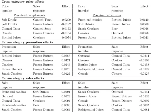
To get more insight in the sign of the cross-category effects, we summarize each IRF by the sum of the first 10 responses, and average this number over all stores. Table 1.7 reports the five largest positive and negative cross-category effects of price, promotion and sales on sales.

(36)

Table 1.6: Size of within and cross-category effects of price, promotion and sales on sales, summed across 10 lags of the IRF, averaged across stores and product categories, and in absolute value.

Within-category 0.004 0.006 0.057

Cross-category 0.002 0.005 0.002

Cross-category price effects. We investigate whether consumers perceive cat-egories as complements or as substitutes. Complementary and substitution ef-fects occur between categories because they are consumed together or separately. Following the standard economic definition [Pashigian, 1998], complements are defined as goods having a negative cross-price elasticity, whereas substitutes are defined as goods having a positive cross-price elasticity. We find evidence of two important drivers of cross-category price effects: consumption relatedness and the budget constraint.

As an example of consumption relatedness, consider Soft Drink prices and Frozen Juices. An increase in Soft Drink prices makes consumers spend more on other drinks as a compensation, in particular Frozen Juices (see Table 1.7). The joint dynamic effect of a one standard deviation price impulse of Soft Drinks on the sales response growth of Frozen Juices is depicted in Figure 1.4 for the first three stores in the data set. Note that the instantaneous effect is estimated as exactly zero since the Sparse VAR puts the corresponding effect in theΣb matrix to

zero. We see a sharp increase in Frozen Juices sales growth one week after the soft drink price increase, indicating substitution. However, the next two weeks, sales growth of Frozen Juices slows down, which could indicate stockpiling behavior [Gangwar et al., 2014].

Another example of consumption relatedness is Soft Drinks and Frozen En-trees. As can be seen from Table 1.7, we find a strong negative effect of Soft Drink prices on Frozen Entrees. This might be due to the fact that Soft Drinks and Frozen Entrees are consumed together. We do not find the opposite effect of price changes in Frozen Entrees on the sales of Soft Drinks. This asymmetry arises because Soft Drinks is a destination category (high influence), while Frozen Entrees is a convenience category (highly responsiveness).

Concerning the budget constraint, prominent cross-category price effects are observed for Soft Drinks and Cereals, both destination categories. Soft Drinks and Cereals account for a relatively large proportion of the expenditures of US

(37)

Table 1.7: Cross-category price, promotion and sales effects on sales summed across 10 lags of IRFs and averaged across stores. We present only the five largest positive and negative effects.

Cross-category price effects

Price Sales Effect Price Sales Effect

impulse response impulse response

Perceived complements Perceived substitutes

Soft Drinks Canned Tuna -0.0209 Front-end-candies Bottled Juices 0.0120

Soft Drinks Frozen Entrees -0.0182 Soft Drinks Frozen Juices 0.0060

Canned Tuna Canned Soup -0.0173 Snack Crackers Beer 0.0058

Cereals Frozen Dinners -0.0104 Cookies Oatmeal 0.0056

Bottled Juices Crackers -0.0074 Frozen Juices Bottled Juices 0.0023

Cross-category promotion effects

Promotion Sales Effect Promotion Sales Effect

Bottled Juices Frozen Entrees 0.0586 Oatmeal Canned Tuna -0.0214

Cheeses Frozen Entrees 0.0421 Cheeses Cookies -0.0160

Crackers Frozen Entrees 0.0246 Bottles Juices Canned Tuna -0.0158

Frozen Dinners Frozen Entrees 0.0170 Refrigerated Juices Canned Tuna -0.0128

Snack Crackers Frozen Entrees 0.0127 Cereals Cheeses -0.0127

Cross-category sales effects

Sales Sales Effect Sales Sales Effect

Front-end-candies Soft Drinks 0.0191 Snack Crackers Oatmeal -0.0154

Oatmeal Frozen Entrees 0.0123 Frozen Juices Frozen Entrees -0.0120

Canned Tuna Crackers 0.0094 Cereals Frozen Dinners -0.0099

Front-end-candies Beer 0.0086 Snack Crackers Cookies -0.0087

Snack Crackers Frozen Dinners 0.0064 Refrigerated Juices Canned Tuna -0.0084

families (respectively 22% and 14% of spending on food and drinks, see Table 1.2), which indicates that the budget constraint is an important source of cross-category effects.

Cross-category promotion effects. The results in Table 1.7 indicate that brand-ing and promotion intensity are important drivers of cross-category promotion effects. Concerning branding, cross-category promotion effects are observed for categories that share brands such as Frozen Dinners and Frozen Entrees (e.g. the frozen prepared foods brand ‘Stouffer’s’). Concerning promotion intensity, promi-nent cross-category promotion effects are observed for categories in which a high percentage of the SKUs is promoted, such as Cheeses and Bottled Juices (respec-tively 28% and 26% of SKUs, on average, are promoted in our data.) A promotion impulse in such categories might either trigger joint consumption (e.g. Bottled Juices and Frozen Entrees), or deter consumption (e.g. Cheeses and Cookies).

(38)

24 Sparse estimation of the VAR 0 2 4 6 8 10 −0.10 −0.05 0.00 0.05 0.10 Store 1 Lag 0 2 4 6 8 10 −0.10 −0.05 0.00 0.05 0.10 Store 2 Lag 0 2 4 6 8 10 −0.10 −0.05 0.00 0.05 0.10 Store 3 Lag

Figure 1.4: Impulse response function: response of frozen juices sales growth to a one standard deviation impulse in the price of soft drinks.

Cross-category sales effects. In Table 1.7, we find evidence of two important drivers of cross-category effects of sales on sales: affinity in consumption and the budget constraint. Prominent cross-category sales effects occur because of affinity in consumption. Some categories are jointly consumed towards a common goal, such as Front-end-candies and Soft Drinks/Beer (for a light meal); while others such as Snack Crackers and Cookies are purchased as replacements since consumers might perceive them to have a similar functionality. Concerning the budget constraint, we find some cross-category sales effects between seemingly unrelated categories such as Refrigerated Juices and Canned Tuna.

Importantly, the results from Table 1.7 are in line with our findings on cat-egory influence and responsiveness. Destination categories such as Soft Drinks, Cereals and Cheeses mainly influence sales in other categories through their price, promotion or sales impulses. Convenience categories such as Frozen Entrees and Frozen Dinners are more responsive to changes in other categories. Routine cat-egories, such as Cookies, are moderately influential and moderately responsive, while occasional categories, such as Oatmeal, are highly responsive.

(39)

1.6.3 Robustness checks

Alternative penalty function. We investigate the robustness of the results to the choice of the penalty function. We re-estimate the models using the Sparse VAR with elastic net instead of the grouplasso penalty (a short explanation of the elastic net is given in Section 1.4). The managerial insights obtained by Sparse VAR with either grouplasso or elastic net are very similar. Similarities are that (i) within-category effects are more common and larger in magnitude than cross-within-category effects, (ii) destination categories such as Cheeses and Cereals are very influential, (iii) convenience categories such as Frozen Entrees, and occasional categories such as Crackers are very responsive (iv) routine categories such as Bottled Juices, Refrigerated Juices and Cookies are both influential and responsive (v) the most prominent cross-category effects of price, promotion and sales on sales are highly overlapping.

Alternative data period. We also check the performance of the Sparse VAR on the post-1994 data. Retailers made extensive use of ‘pay-for-performance’ price promotions that are not fully reflected in the Dominick’s database. The data generating process might have changed in this period. Therefore, we should not assume constant parameter values. We re-estimate the model on the post-1994 data (data from October 1995 until May 1997) and verify its performance. In the post-1994 period, similar conclusions can be drawn with respect to within versus cross-category effects and category influence and responsiveness. Some differences are observed in the post-1994 period concerning the impulse response functions. These differences occur due to an altered strategy concerning average pricing and promotion intensity in the 17 product categories in the post-1994 period compared to the 1993-1994 period. Detailed results are available from the authors upon request.

Alternative price time series. We investigate the robustness of the results to the calculation of the price time series. Instead of aggregating prices from the SKU level to the product category level using SKU market shares as weights (cfr. Section 1.5), we now take the normal mean over all SKUs. We re-estimate the model using the newly calculated price time series. Similar insights are obtained with respect to cross-category effects and category influence and responsiveness. The most influential categories in the cross-category network of prices on sales are the destination categories Cereals and Cheeses; the most responsive ones the convenience categories Frozen Entrees, Frozen Dinners and Canned Tuna.

(40)

Table 1.8: Mean Absolute Forecast Error (MAFE) for category-specific sales, averaged over the 15 stores and the 17 product categories. P-values of a Diebold-Mariano test comparing the Sparse VAR to its alternatives are indicated between parentheses.

Sparse VAR LS Restricted LS Bayesian Methods 1-step Iterative Minnesota NIW MAFE 736.80 1298.54

(<0.01) 784(<0..01)96 734(0.38).82 875(<0..01)47 1078(<0.01).03

select the penalty parameters. We also ran the analysis using AIC as a selection criterion for the penalty function. While the model selected by AIC are slightly less sparse, the substantive insights do not change.

1.6.4 Forecast Performance

Although prediction is not the main goal of the proposed methodology, we deem it important to show that the Sparse VAR can compete with other methods in terms of prediction accuracy. We estimate model (1.6) for each store and perform a forecast exercise (cfr. Section 1.4), using a rolling window of length S = 67. One-step-ahead forecasts of sales for each product category are computed for

t =S, . . . , T −1, withT = 77. The same estimation methods as in Section 1.4 are used.

Results on the sales predictions are summarized in Table 1.8 by the Mean Absolute Forecast Error (MAFE), averaged across time and over the 17 product categories and 15 stores. The MAFE should be seen as a measure of forecast accuracy, not as a measure of managerial relevance of the obtained results. The variable selection methods Sparse VAR, 1-step and Iterative Restricted LS per-form, on average, better than the methods that do not perform variable selection. This indicates that sparsity improves prediction accuracy. Sparse VAR and Itera-tive Restricted LS achieve the best forecasting performance. A Diebold-Mariano test confirms that latter two methods significantly outperform the other methods. We conclude that the improvement in interpretability of the model obtained by Sparse VAR, as discussed in the previous section, does not come at the cost of lower forecast performance.