Title Page
Differential Item Functioning for Polytomous Response Items Using Hierarchical Generalized Linear Model
by
Meng Hua
B.S., Southwest University of China, 2008 M.S., State University of New York at Albany, 2010
Submitted to the Graduate Faculty of the School of Education in partial fulfillment
of the requirements for the degree of Doctor of Philosophy
University of Pittsburgh 2019
COMMITTEE PAGE
UNIVERSITY OF PITTSBURGH SCHOOL OF EDUCATION
This dissertation was presented by
Meng Hua
It was defended on October 31, 2019
and approved by
Clement A. Stone, PhD, Professor, Department of Psychology in Education Lan Yu, PhD, Associate Professor, Department of Medicine
Dissertation Advisor: Feifei Ye, PhD, Senior Scientist, RAND Corporation, Pittsburgh Suzanne Lane, PhD, Professor, Department of Psychology in Education
Copyright © by Meng Hua 2019
Abstract
Differential Item Functioning for Polytomous Response Items Using Hierarchical Generalized Linear Model
Meng Hua, PhD
University of Pittsburgh, 2019
Hierarchical generalized linear model (HGLM) as a differential item functioning (DIF) detection method is a relatively new approach and has several advantages; such as handling extreme response patterns like perfect or all-missed scores and adding covariates and levels to simultaneously identify the sources and consequences of DIF. Several studies examined the performance of using HGLM in DIF assessment for dichotomous items, but only a few exist for polytomous items. This study examined the DIF-free-then-DIF strategy to select DIF-free anchor items and the performance of HGLM in DIF assessment for polytomous items. This study extends the work of Williams and Beretevas (2006) by adopting the constant anchor item method as the model identification method for HGLM, and examining the performance of DIF evaluation with the presence of latent trait differences between the focal and reference group. In addition, the study extends the work of Chen, Chen, and Shih (2014) by exploring the performance of HGLM for polytomous response items with 3 response categories, and comparing the results to logistic regression and Generalized Mantel-Haensel (GMH) procedure.
In this study, the accuracy of using iterative HGLM with DIF-free-then-DIF strategy to select DIF-free items as anchor was examined first. Then, HGLM with 1-item anchor and 4-item anchor were fitted to the data, as well as the logistic regression and GMH. The Type I error and power rates were computed for all the 4 methods. The results showed that compared to dichotomous items, the accuracy rate of HGLM methods in selecting DIF-free item was generally
lower for polytomous items. The HGLM with 1-item and 4-item anchor methods showed decent control of Type I error rate, while the logistic regression and GMH showed considerably inflated Type I error. In terms of power, HGLM with 4-item anchor method outperformed the 1-item anchor method. The logistic regression behaved similarly to HGLM with 1-item anchor. The GMH was generally more powerful, especially under small sample size conditions. However, this may be a result of its inflated Type I error. Recommendations were made for applied researchers in selecting among HGLM, logistic regression, and GMH for DIF assessment of polytomous items.
Table of Contents
Preface ... xv
1.0 Introduction ... 1
1.1 Background ... 1
1.1.1 DIF assessment for polytomous items ... 2
1.1.2 DIF assess under hierarchical generalized linear model framework ... 4
1.2 Statement of the Problem ... 6
1.3 Purpose of the Study ... 8
1.4 Research Questions ... 8
1.5 Significance of the Study ... 9
1.6 Organization of the Study ... 9
2.0 Literature Review ... 10
2.1 DIF Assessment Methods for Polytomous Items ... 10
2.1.1 Nonparametric methods ... 11
2.1.1.1 The Mantel test ... 11
2.1.1.2 Standardized mean difference (SMD) statistic ... 13
2.1.1.3 Generalized Mantel-Haenszel (GMH) ... 14
2.1.2 Parametric methods ... 15
2.1.2.1 Polytomous logistic regression (PLR) ... 16
2.1.2.2 Polytomous logistic discriminant function analysis (LDFA) ... 18
2.1.2.3 IRT likelihood-ratio test (IRT-LR) ... 19
2.1.4 Factors considered in DIF detection studies ... 23
2.1.4.1 Examinee factors ... 23
2.1.4.2 Test factors ... 25
2.1.4.3 DIF factors ... 26
2.2 DIF Assessment Using HGLM ... 28
2.2.1 A HGLM framework for DIF ... 28
2.2.2 Model identification ... 32
2.2.3 Performance of HGLM in DIF detection ... 33
2.3 DIF Assessment with Rating Scale ... 37
3.0 Method ... 39
3.1 Fixed Factors ... 40
3.1.1 Scale length ... 40
3.1.2 Item discrimination parameter α ... 40
3.1.3 Model identification method ... 41
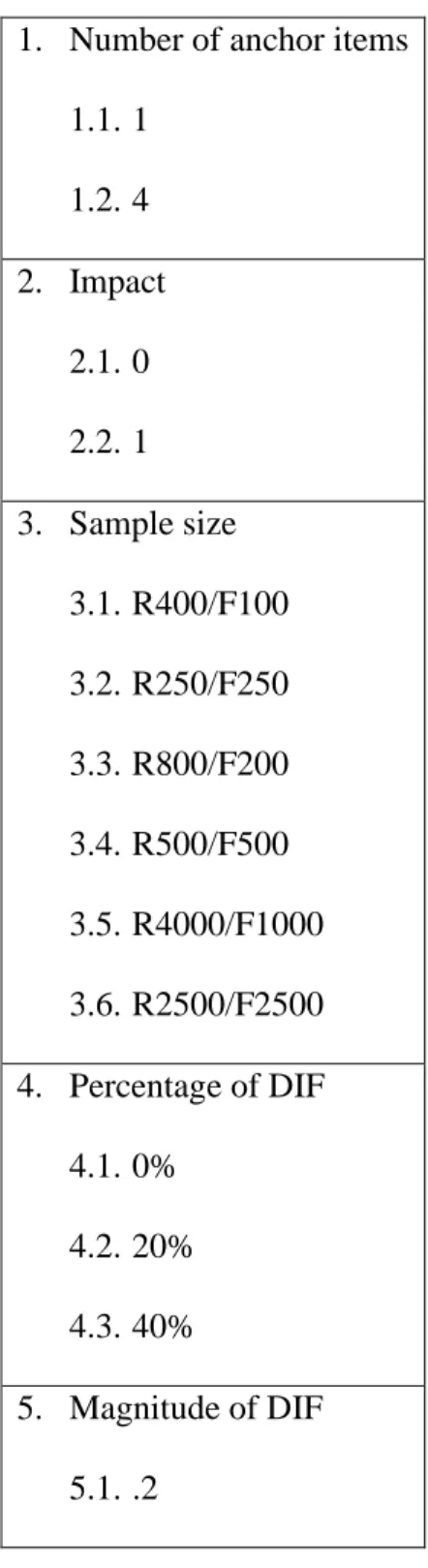
3.2 Manipulated Simulation Conditions ... 42
3.2.1 Anchor items ... 42
3.2.2 Latent trait parameter difference between groups and impact (0, 1) ... 44
3.2.3 Sample size and sample size ratio ... 45
3.2.4 Percentage of DIF items (0%, 20%, and 40%) ... 46
3.2.5 Magnitude of DIF (.2, .6) ... 46
3.2.6 DIF patterns (constant, balanced, unbalanced) ... 47
3.3 Evaluation Criteria ... 50
3.3.2 Type I error rate... 50
3.3.3 Statistical power ... 51
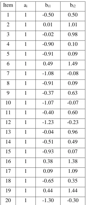
3.4 Data Generation and Validation ... 51
3.4.1 Data generation ... 51
3.4.2 Data validation ... 53
3.5 Data Analysis ... 55
3.5.1 Estimation methods ... 55
3.5.2 Generalized Mantel-Haenszel and polytomous logistic regression ... 56
4.0 Results ... 57
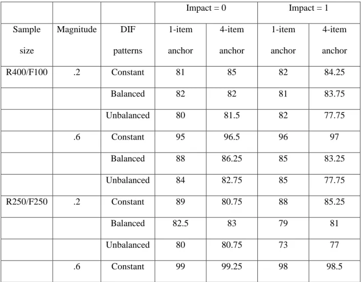
4.1 Results of Study 1 ... 57
4.1.1 Accuracy rates of using HGLM to select DIF free items ... 58
4.1.2 ANOVA results of study 1 ... 61
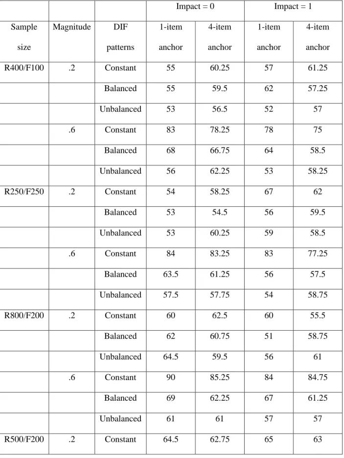
4.2 Results of Study 2: Type I Error ... 66
4.2.1 Results of Type I error rates ... 67
4.2.2 ANOVA results of Type I error ... 70
4.3 Results of Study 2: Power ... 82
4.3.1 Results of Power ... 82
4.3.2 ANOVA results of Power... 85
4.4 Summary of the Results for Study 2 ... 93
5.0 Discussion... 99
5.1 Major Findings and Implications ... 99
5.1.1 Answers to research questions ... 99
5.1.3 Conclusion ... 108
5.2 Limitations and Future Research ... 110
Appendix A Detailed Results for Study 1 ... 112
Appendix B Detailed Results for Study 2 ... 126
Appendix B.1 Results for Type I Error ... 126
Appendix B.2 Results for Power ... 138
Appendix C SAS Syntax Sample ... 149
Appendix C.1 Sample Syntax for Study 1 ... 149
Appendix C.2 Sample Syntax for Study 2 ... 150
List of Tables
Table 1 Data for the kth Level of a 2×T Contingency Table Tsed in DIF Tetection ... 10
Table 2 Specifications of Simulation Conditions... 49
Table 3 Item Parameters for Data Generation for the Reference Group ... 52
Table 4 Estimated θ for the no impact and impact groups ... 53
Table 5 Generated item parameters for the focal and reference groups when impact = 0 .. 54
Table 6 Accuracy (%) of Selecting DIF-Free Items as Anchor with 20% DIF Items ... 58
Table 7 Accuracy (%) of Selecting DIF-Free Items as Anchor with 40% DIF Items ... 60
Table 8 Mean and Standard Deviation of Accuracy for Pattern, Percentage and Magnitude of DIF ... 62
Table 9 Mean and Standard Deviation of Type I Error Rates for Method, Sample Size and DIF Patterns ... 75
Table 10 Mean and Standard Deviation of Type I Error Rates for Method, Sample Size and % of DIF ... 77
Table 11 Mean and Standard Deviation of Type I Error Rates for Method, Sample Size and Manitude of DIF ... 78
Table 12 Mean and Standard Deviation of Type I Error Rates for Method, DIF Pattern and Percentage of DIF ... 79
Table 13 Mean and Standard Deviation of Type I Error Rates for Method, Magnitude and Percentage of DIF ... 80
Table 14 Mean and Standard Deviation of Type I Error Rates for Method, DIF Pattern and Magnitude of DIF ... 81
Table 15 Mean and Standard Deviation of Power for Method, Sample Size and DIF Patterns ... 89 Table 16 Mean and Standard Deviation of Power for Method, Sample Size and Manitude of DIF ... 90 Table 17 Mean and Standard Deviation of Power for Method, DIF Pattern and Percentage of DIF ... 91 Table 18 Mean and Standard Deviation of Power for Method, DIF Pattern, and Magnitude
of DIF ... 92
Appendix Table 1 Means and Standard Deviations for the Accuracy of Selecting DIF Items ... 112 Appendix Table 2 ANOVA Results for the Accuracy of Selecting DIF Items ... 114 Appendix Table 3 Simple Comparison for the Accuracy of Selecting DIF Items, DIF Pattern by Sample Size ... 115 Appendix Table 4 Simple Comparison for the Accuracy of Selecting DIF Items, DIF Pattern by Percentage of DIF Items ... 116 Appendix Table 5 Simple Comparison for the Accuracy of Selecting DIF Items, DIF Pattern
by Magnitude of DIF Items ... 117 Appendix Table 6 Simple Comparison for the Accuracy of Selecting DIF Items, Percentage
of DIF by Magnitude of DIF Items ... 118 Appendix Table 7 Means And Standard Deviations for The Accuracy of Selecting DIF Items, DIF Pattern by Sample Size ... 119 Appendix Table 8 Means and Standard Deviations for the Accuracy of Selecting DIF Items, DIF Pattern by Percentage of DIF Items ... 120
Appendix Table 9 Means and Standard Deviations for the Accuracy of Selecting DIF Items,
DIF Pattern by Magnitude of DIF Items ... 121
Appendix Table 10 Means and Standard Deviations for the Accuracy of Selecting DIF Items, Percentage of DIF Items by Magnitude of DIF ... 121
Appendix Table 11 Mean Type I Error Rates (%), without Impact... 126
Appendix Table 12 Mean Type I Error Rates (%), with Impact = 1 ... 130
Appendix Table 13 Means and Standard Feviations for the Type I Error Rates... 134
Appendix Table 14 ANOVA Results for Type I Error Rates ... 136
Appendix Table 15 Mean Power Rates (%), without Impact ... 138
Appendix Table 16 Mean Power Rates (%), with Impact = 1 ... 142
Appendix Table 17 Means and Standard Deviations for Power ... 146
List of Figures
Figure 1 Three-way Interaction of Accracy among Pattern, Percentage, and Magnitude of DIF ... 62 Figure 2 Type I error Rates for All Conditions ... 69 Figure 3 Three-Way Interaction of Type I Error among Methods, Sample Size and DIF
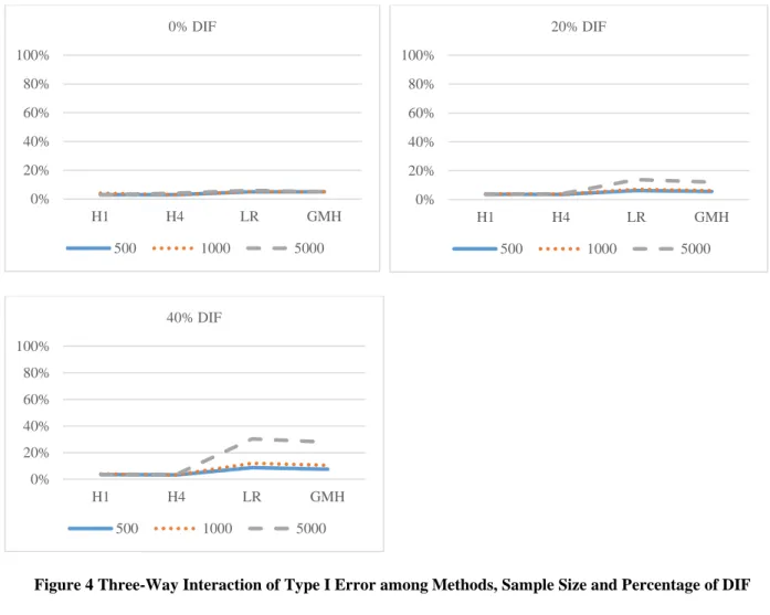
Pattern ... 74 Figure 4 Three-Way Interaction of Type I Error among Methods, Sample Size and
Percentage of DIF ... 76 Figure 5 Three-Way Interaction of Type I Error among Methods, Sample Size and
Magnitude of DIF ... 78 Figure 6 Three-Way Interaction of Type I Error among Methods, DIF pattern and
Percentage of DIF ... 79 Figure 7 Three-Way Interaction of Type I Error among Methods, Magnitude and Percentage of DIF ... 80 Figure 8 Three-Way Interaction of Type I Error among Methods, DIF Pattern and
Magnitude of DIF ... 81 Figure 9 Power for All Conditions ... 84 Figure 10 Three-way Interaction of Power oor the Method, Sample Size, and DIF Pattern
... 88 Figure 11 Three-way Interaction of Power for the Method, Sample Size, and Magnitude of DIF ... 90
Figure 12 Three-Way Interaction Of Power For The Method, DIF Pattern, and Percentage Of DIF ... 91 Figure 13 Three-way Interaction of Power for the Method, DIF Pattern, and Magnitude of DIF ... 92 Figure 14 Type I Error and Power Rates for Sample Size and DIF Pattern for HGLM with 4-item Anchor and GMH ... 95 Figure 15 Type I Error and Power Rates for Sample Size and Magnitude of DIF for HGLM
with 4-item Anchor and GMH ... 96 Figure 16 Type I Error and Power Rates for DIF Pattern and Percentage of DIF for HGLM
with 4-item Anchor and GMH ... 97 Figure 17 Type I Error and Power Rates for DIF Pattern and Magnitude of DIF for HGLM with 4-item Anchor and GMH ... 98 Appendix Figure 1 Two-way Interaction of Accuracy between DIF Pattern and Sample Size ... 122 Appendix Figure 2 Two-way Interaction of Accuracy between DIF Pattern and Percentage of DIF Items ... 123 Appendix Figure 3 Two-way Interaction of Accuracy between DIF Pattern and Magnitude
of DIF Items ... 124 Appendix Figure 4 Two-way Interaction of Accuracy between Percentage and Magnitude of
Preface
The road to a doctorial degree is long and hard, and I would never have made it without the help and support of my advisor and friend Dr. Feifei Ye. I cannot thank her enough. I would also like to thank Dr. Suzanne Lane, Dr. Clement Stone, and Dr. Lan Yu, for the guidance and insight they provided while on my dissertation committee. And Dr. Kevin Kim, whom I miss to this day.
I must also thank my dear parents, whose unconditional love and support make me who I am. And my cat Captain Blue. D. McMeowmers, although utterly unhelpful, but her company got me through all those long dark nights.
1.0Introduction
1.1Background
For the past few decades, measurement equivalence has been an increasing concern in psychological and health studies. If measurement bias is present, a measurement scale is no longer invariant across groups, which means the measures perform differently for different groups of participants, thereby threatening cultural fairness and the accurate estimation of treatment effects, and may lead to flawed public policies (McHorney & Fleishman, 2006). Measurement equivalence can be viewed from various perspectives (Borsboom, 2006); it is often examined under the item response theory (IRT) framework, which is essentially an examination of differential item functioning (Embretson & Reise, 2000).
Differential item functioning (DIF) refers to a situation in which an item functions differently in two groups of participants conditioned by the latent measured trait. The presence of DIF is an indication of measurement bias; over the years, it has rendered concerns from numerous researchers. DIF assessment has a long history in education testing and is well-developed for dichotomous response items, possibly due to the popularity of multiple choice items that are scored as correct or incorrect, but it is less so for polytomous response items, which are scored on multiple points.
DIF assessment, although originated in education testing, is now becoming popular in health studies (Teresi, 2006). McHorney and Fleishman (2006) argued that DIF assessment is fundamental to health-related studies; as modern society becomes more culturally diverse in its age, racial, and socioeconomic status composition, it is crucial that health-related outcome
instruments are culturally fair. In 2017, a search of PubMed using the term “differential item functioning” resulted in 1271 articles, while in 2010, Scott et al. (2010) conducted a similar search that resulted in 211 articles. Researchers have been using DIF to evaluate the performance of measurement scales across participants of different age, gender, race, language, country, socioeconomic status, education, employment status, health care settings, and other characteristics. DIF has been identified in many health-related areas, such as mental health status, physical functioning and functional ability, patient satisfaction, and quality of life (McHorney & Fleishman, 2006; Scott, et al, 2010). Polytomous items are common in psychological evaluations and health studies, as the instruments often employ a Likert-scale type of measure. Therefore, researchers have been increasingly interested in DIF assessment for polytomous items.
1.1.1 DIF assessment for polytomous items
DIF assessment for polytomous items, however, presents its unique challenges. Penfield and Lam (2000) discussed three issues pertaining to the extension of DIF assessment from dichotomous items to polytomous items. First, reliabilities are typically lower in polytomous items. This effect results from a combination of shorter scale length, inconsistency of the rater scores, and more dissimilar content domains, all of which are common in polytomous items. Lower reliability is often related to inaccuracies in the trait estimates, which leads to false identification of DIF items, known as the Type I error.
Second, DIF assessment requires a matching variable to match examinees from the focal and reference groups with equal levels of latent trait so they are comparable. Traditionally, this is done by using the total score or some function of the total score as the matching variable. There are two classes of DIF procedures: the observed score approach uses the observed score as the
matching variables, while the latent trait approach uses an estimate of latent trait, which is a function of the observed score (Potenza & Dorans, 1995). The matching variable should be a sufficient estimate of the trait; in other words, information in the latent trait variable should be captured by the matching variable. In addition, the matching variable should be a reliable estimate of the latent trait (Meredith & Millsap, 1992). A mismatch between the latent trait and observed scores can inflate Type I error with the presence of different group abilities or trait levels (DeMars, 2010). However, due to the typically shorter scale length, lower reliability, and potential multidimensionality, defining a matching variable is less straightforward for polytomous items (Zwick, Donoghue, & Grima 1993).
One possible solution is using an external criterion to match the groups of examinees (Zwick, et al., 1993), as the chosen external variable can have high reliability. However, the main problem with this approach is that the external matching variable is not necessarily highly correlated with the target test; in other words, the external matching variable and the target test may not be measuring the same construct. Another solution is to improve the performance of the matching variable. Zwick et al. (1993) suggested including the studied item in the matching variable. Purifying the matching variable has also been found to result in more accurate results in polytomous DIF assessment (Hildago-Montesinos & Gómez-Benito, 2003; Su & Wang, 2005). Another way is to use a matching variable based on the estimated latent trait instead of the observed score (DeMars, 2008).
Third, creating a measure of item performance is more complex for polytomous items. For dichotomous items, item performance can be assessed by estimating the probability of a correct response. However, for polytomous items with multiple response categories, there is no single
measure, but rather, several degrees of correct response; in addition, there is a potential group difference in each category of response.
There are several solutions to this problem. One approach is to place the polytomous responses on an interval scale and compare the group mean score at each level of a matching variable, as adopted by the Mantel test (Mantel, 1963), and standardized mean difference (SMD) statistic (Dorans & Schmitt, 1991). The major problem with this approach lies in the appropriateness of treating ordinal responses on an interval scale. Sometimes the score categories may be nominal in nature, meaning the adjacent categories do not necessarily represent ordered levels of performance, making this approach more problematic. Another approach is to test for the group-by-score dependence at each level of matching variable, thus preserving the categorical nature of the rating scales. This is the method adopted by the generalized Mantel-Haenszel (GMH) approach (Somes, 1986). A third approach is to dichotomize the polytomous scale using various strategies and to assess the group difference in odds of a certain response as in the dichotomous scale. This is the logic used by the polytomous logistic regression procedure (PLR) (Agresti, 2013; French & Miller, 1996). The Mantel test, SMD and GMH do not specify a parametric form to match the item score at each trait level; this is known as the nonparametric method. As the logistic type of procedures do specify a parametric form to match item score at each trait level using a mathematical function, they are known as the parametric method.
1.1.2 DIF assess under hierarchical generalized linear model framework
One of the relatively new methods for DIF assessment is to use the hierarchical generalized linear model, which has received increasing attention. The hierarchical generalized linear model (HGLM), also known as the generalized linear mixed model, is a general form for nested data that
models nonlinear relationships. The popular hierarchical linear model (HLM) is a special case of HGLM in which the sampling data is normal, the link function is canonical, and the structure model is linear (Raudenbush & Bryk, 2002).
The relationship between IRT and HGLM has long been demonstrated by various researchers (Adams, Wilson, & Wu, 1997; Kamata, 2001). Kamata (2001) showed that the Rasch model is mathematically equivalent to a 2-level HGLM with fixed item parameters and random person parameters. Items are treated as repeated measures nested within participants. Willams and Beretvas (2006) expanded Kamata’s work and demonstrated the equivalence of polytomous HGLM and a constrained form of Muraki’s rating scale model. Since then, researchers have examined the HGLM for accounting for item dependence (Beretvas & Walker, 2012; Fukuhara & Paek, 2015; Paek & Fukuhara, 2015; Xie, 2014), and to account for both person and item dependence (Jiao, Kamata, Wang, & Jin, 2012; Jiao & Zhang, 2015).
HGLM has several advantages over the traditional IRT approach for DIF evaluation. First, in the HGLM framework, DIF can be interpreted as the difference between item parameter estimates in the focal group and the reference group, specified as the cross-level interactions between group indicators and item parameters (Chen, Chen, Shih, 2014); thus, the model allows assessment of multiple sources of DIF by examining the variability of DIF across items(Beretvas, Cawthon, Lockhart & Kaye, 2012; Van den Noortgate & De Boeck, 2005). Furthermore, additional covariates can be incorporated into the model to provide alternate explanations for DIF, rather than the descriptive measurement approach that the traditional IRT model takes, which focuses on the performance of the scale at measuring the participant’ trait level (De Boeck & Wilson, 2004; Swanson, Clauser, Case, Nungester & Featherman, 2002). Thus, the model is more general, flexible, and conceptually useful. Second, the extreme response patterns of perfect scores
and all-missed scores can both be used for parameter estimation. Third, examination of the variability in person-level scale scores allows researchers to explore the consequences of DIF (Cheong & Kamata, 2013). Fourth, additional levels can be added to the model to account for higher-level clusters, such as doctor or hospital, while studies have shown that ignoring such nested structures can yield consequences such as inflated Type I error rate (French & Finch, 2010). Last, implementation of HGLM is more straightforward with widely available software. In addition, HGLM and its extensions can simultaneously handle item and person parameters, DIF, effect of covariates, as well as local item and person dependence. Thus, it has great potential for practical use (Ravand, 2015).
1.2Statement of the Problem
One of the common issues for DIF detection is scale indeterminacy. Scale indeterminacy refers to the estimation of a DIF parameter that is not absolute but related to the other DIF parameters in the same scale (de Ayala, 2009). In order to solve this problem, it is necessary to set constraints to identify the model. Most studies that address this issue are in education testing settings. There are three popular approaches: the mean of the person ability parameter or the mean of the item difficulty parameter can be constrained to an arbitrary value (e.g., zero), or a set of anchor items can be selected to serve as a matching criterion variable (Chen et, al, 2014; Wang, 2004). Some studies examined the effect of different constraining methods using HGLM on DIF detection for dichotomous items. Cheong and Kamata (2013) explored the performance of the equal mean difficulty method and the constant anchor item method and compared the results to the well-researched Mantel-Haenszel procedure. Chen et al. (2014) explored the performance of
the equal mean ability method with rank-based strategy (Woods, 2009) and the constant anchor item method with the DIF-free-then-DIF strategy (DFTD; Wang, Shih, & Sun, 2012) for two criteria: first the accuracy in selecting DIF-free items, and then for Type I error rate and power. They found that the equal mean ability method is sensitive to group difference in ability (usually referred to as “impact”) and is prone to Type I error under such conditions. As a result, it is not recommended if researchers suspect impact might be present (Chen et al., 2014). The equal mean difficulty method is more robust than the constant anchor item method when there is a violation of assumptions. Thus, it is recommended by Cheong and Kamata (2013). If the constant anchor item method is to be used, it is important that procedures be completed to make sure the reference items selected are free of DIF. However, these studies focused only on dichotomous items, not on polytomous items.
With polytomous items, literature examining the performance of HGLM in DIF assessment is relatively scarce. As previously mentioned, Willams and Beretvas (2006) extended Kamata’s (2011) dichotomous HGLM to polytomous items and demonstrated the mathematical equivalence between Muraki’s rating scale model (Muraki, 1990) and polytomous HGLM. The authors compared the performance of HGLM and IRT models for parameter recovery and found the two performed similarly. A comparison between HGLM and the generalized Mantel-Haenszel (GMH) approach for DIF detection under the condition of no group ability difference showed the two approaches produced similar results in terms of Type I error rate and statistical power. Ryan (2008) extended this study and found similar results. However, these studies used equal mean person ability method to constrain the model; in addition, the ability of groups of examinees was set to be equal, meaning no impact among groups. Yet impact is most likely present in reality, and plays an
important role in DIF assessment. It is necessary to extend these studies by exploring the performance of HGLM with different constraining methods, as well as with the presence of impact.
1.3Purpose of the Study
The purpose of this study is to evaluate the performance of HGLM in DIF assessment for polytomous items, and in comparison to the GMH and polytomous logistic regression procedures. Specifically, this study expanded the work of Chen et al. (2014) by applying HGLM with DFTD strategy to polytomous items, using the constant anchor item method. Additionally, this study expanded the work of Williams and Beretvas (2006) by exploring the performance of DIF with the presence of impact.
1.4Research Questions
This study attempted to answer the following three questions:
1. How accurately can HGLM select DIF-free items as anchor items for DIF analysis? 2. What is the Type I error rate for DIF detection using HGLM, and how does it compare to
using GMH and logistic regression?
3. What is the statistical power for DIF detection using HGLM, and how does it compare to using GMH and logistic regression?
1.5Significance of the Study
DIF assessment, as a tool to evaluate item fairness, is an integrated part of health studies. As the instruments in health studies commonly employ a Likert-type of scale, researchers have been paying more attention to DIF assessment for polytomous items, which is less developed and studied than DIF assessment for dichotomous items. DIF assessment with HGLM is a relatively new approach; in previous studies it has been proved useful for dichotomous items and showed great potential for polytomous items. However, the performance of HGLM in DIF assessment for polytomous items is not yet fully understood. This dissertation study aims to provide more information on this subject and produce useful guidelines for practitioners.
1.6Organization of the Study
The rest of this dissertation is organized as follows: the second chapter reviews DIF assessment for polytomous items and various detection methods followed by an introduction of using HGLM and its application for DIF detection. The third chapter describes the Monte Carlo study in detail; simulation factors, evaluation criteria, data generation, validation, and analysis are discussed. The fourth chapter reports the results, and the fifth chapter summarizes and discusses the findings.
2.0Literature Review
This chapter consists of several sections reviewing literature on DIF assessment on polytomous response items under the HGLM framework. First, DIF assessment for polytomous response items was reviewed; then, DIF detection using HGLM were discussed.
2.1DIF Assessment Methods for Polytomous Items
To formulate DIF for polytomous items, assume y1, y2, …, yt as the T scores of a certain
item, where T is the number of possible response category scores. Reference and focal groups are noted as F and R. K is the number of levels of stratification variable. Table 1 presented a 2×T contingency table for the kth stratum, with the row and column marginal totals fixed.
Table 1 Data for the kth Level of a 2×T Contingency Table Tsed in DIF Tetection
Group Item Score Total
y1 y2 … yt … yT
Reference nRIk nR2k nRtk nRTk nR+k
Focal nFIk nF2k nFtk nFTk nF+k
2.1.1 Nonparametric methods
Methods such as the Mantel, SMD and GMH approaches do not assume a particular statistical model to link item scores to the matching variable; instead, they just focus on the group difference in the observed item scores at each level of the matching variable; thus they are known as nonparametric methods (Penfield & Lam, 2000).
2.1.1.1The Mantel test
The Mantel test is a polytomous extension of the Mantel-Haenszel (MH) procedure, which is one of the most widely-used DIF detection methods. MH for dichotomous items utilizes a series of K 2×2 contingency tables for each scoring level after examinees in both groups are matched on the total scores; where K is the number of the levels of the matching variable (Mantel & Haenzel, 1959). The Mantel test extended the MH by using a series of K 2×T tables with 2 rows and T columns, where T is the number of possible response category scores (Mantel, 1963). The test statistic is created by calculating weighted sum scores for the focal group and then summed for each response, conditioning on the total test score. Each table is created for each stratum of ability level. The null hypothesis is that the odds of correct response are the same in both the focal and the reference groups.
The weighted sum of scores for the focal group in the kth table for the kth stratum is Fk = ∑𝑇𝑇𝑡𝑡=1𝑦𝑦𝑡𝑡𝑛𝑛𝐹𝐹𝑡𝑡𝐹𝐹 (1)
where yt is the item score for the T possible score on the item. nFtk is the number of focal group
members with score t in the kth stratum. Under the hypothesis of no association, the rows and columns are considered independent; thus the rows and columns of frequencies for each group are
distributed as multivariate hypergeometric variables; that is, nFk is a multivariate hypergeometric
variable with parameters nF+k while n+k with parameters n++k. Thereby the expected value of Fk is
E(Fk) = 𝑛𝑛𝑛𝑛𝐹𝐹+𝑘𝑘
++𝑘𝑘∑ 𝑦𝑦𝑡𝑡𝑛𝑛𝐹𝐹𝑡𝑡𝐹𝐹
𝑇𝑇
𝑡𝑡=1 (2)
where a plus sign (+) indicates marginal sums meaning summation over the index; for example, nF+k represents summation over all the numbers of focal group members in the kth score level.
The variance of Fk is V(Fk) = 𝑛𝑛𝑅𝑅+𝑘𝑘𝑛𝑛𝐹𝐹+𝑘𝑘 𝑛𝑛++𝑘𝑘2 (𝑛𝑛++𝑘𝑘−1)[(𝑛𝑛++𝐹𝐹∑ 𝑦𝑦𝑡𝑡 2𝑛𝑛 +𝑡𝑡𝐹𝐹 𝑇𝑇 𝑡𝑡=1 )−(∑𝑇𝑇𝑡𝑡=1𝑦𝑦𝑡𝑡𝑛𝑛+𝑡𝑡𝐹𝐹)2] (3)
Under the hypothesis of no association, the frequency counts can be viewed as following a multivariate hypergeometric distribution, and a chi-square test can be conducted to test the hypothesis, where the test statistic is distributed as a chi-square variable with 1 degree of freedom. To test the null hypothesis, a chi-square statistic is
χ2 = [∑𝐾𝐾𝑘𝑘=1𝐹𝐹𝑘𝑘− ∑𝐾𝐾𝑘𝑘=1𝐸𝐸(𝐹𝐹𝑘𝑘)]2
∑𝐾𝐾𝑘𝑘=1𝑉𝑉(𝐹𝐹𝑘𝑘) (4) with 1 degree of freedom for the χ2 statistic.
A rejection of the null hypothesis provides evidence that even after the focal and
reference group members are matched on the stratification variable of trait measures, there is still a group difference in the responses, indicating the presence of DIF. The Mantel test is easy to compute; however, it is designed to detect uniform DIF. Uniform DIF refers to a DIF when there is no interaction effect between group membership and item performances. In other words, the group difference in the measured property is constant among trait levels (Mellenbergh, 1982). The Mantel test is not defined for DIF with interactions between group membership and item performances (i.e., nonuniform DIF). A measure of overall DIF can be developed using odds ratios as described by Zwick et al. (1993) and Liu & Agresti (1996).
2.1.1.2Standardized mean difference (SMD) statistic
SMD was originally proposed to condense information into a single value for dichotomous items (Dorans & Kulick, 1983, 1986). The null hypothesis is at each level of the matching variable, there is no group difference in proportion of the correct response, which is equivalent to the null hypothesis used by MH statistics (Dorans & Holland, 1993; Potenza & Dorans, 1995). Weighted difference in expected item scores are summed over levels of the matching variables to form DIF statistics.
Zwick & Thayer (1996) extended SMD to polytomous items using the standardized expected item score; the mean item score for each stratum is weighted by the proportion of focal or reference group members at the stratum. The authors presented two different types of standard error; the hypergeometric version was recommended because of the superior performance over the independently distributed multinomial version in terms of standard error ratios. Thereby the DIF statistics can be tested on a standard normal variable. SMD is closely related to the Mantel; both focus on expected test scores at each level of the matching variable.
Using the notations of Table 1, the test statistic for SMD is expressed as SMD = [∑ 𝑛𝑛𝐹𝐹+𝑘𝑘 𝑛𝑛𝐹𝐹++ ∑𝑇𝑇𝑡𝑡=1𝑦𝑦𝑡𝑡𝑛𝑛𝐹𝐹𝑡𝑡𝑘𝑘 𝑛𝑛𝐹𝐹+𝑘𝑘 𝐾𝐾 𝐹𝐹=1 ]-[∑ 𝑛𝑛𝑛𝑛𝐹𝐹+𝑘𝑘𝐹𝐹++∑ 𝑦𝑦𝑡𝑡𝑛𝑛𝑅𝑅𝑡𝑡𝑘𝑘 𝑇𝑇 𝑡𝑡=1 𝑛𝑛𝐹𝐹+𝑘𝑘 𝐾𝐾 𝐹𝐹=1 ] (5)
under the hypergeometric framework of Mantel (1963), and under the null hypothesis Var (Fk) =
Var(Rk); thus the covariance between Fk and Rk is expressed as
Cov(Fk, Rk) = Cov (∑𝑇𝑇𝑡𝑡=1𝑦𝑦𝑡𝑡𝑛𝑛𝐹𝐹𝑡𝑡𝐹𝐹,∑𝑇𝑇𝑡𝑡=1𝑦𝑦𝑡𝑡(𝑛𝑛+𝑡𝑡𝐹𝐹− 𝑛𝑛𝐹𝐹𝑡𝑡𝐹𝐹) (6)
= - ∑𝑇𝑇𝑡𝑡=1𝑦𝑦𝑡𝑡2𝑉𝑉𝑉𝑉𝑉𝑉(𝑛𝑛𝐹𝐹𝑡𝑡𝐹𝐹) = - Var(Fk)
Var(SMD) = ∑ 𝑛𝑛𝐹𝐹+𝑘𝑘 𝑛𝑛𝐹𝐹++ 2 [�𝑛𝑛1 𝐹𝐹+𝑘𝑘� 2 𝑉𝑉𝑉𝑉𝑉𝑉(𝐹𝐹𝐹𝐹) + �𝑛𝑛𝑅𝑅+𝑘𝑘1 � 2 𝑉𝑉𝑉𝑉𝑉𝑉(𝑅𝑅𝐹𝐹)− 𝐾𝐾 𝐹𝐹=1 2�𝑛𝑛1 𝐹𝐹+𝑘𝑘� � 1 𝑛𝑛𝑅𝑅+𝑘𝑘� 𝐶𝐶𝐶𝐶𝐶𝐶(𝐹𝐹𝐹𝐹,𝑅𝑅𝐹𝐹)] = ∑ 𝑛𝑛𝐹𝐹+𝑘𝑘 𝑛𝑛𝐹𝐹++ 2 �𝑛𝑛1 𝐹𝐹+𝑘𝑘+ 1 𝑛𝑛𝑅𝑅+𝑘𝑘� 2 𝑉𝑉𝑉𝑉𝑉𝑉(𝐹𝐹𝐹𝐹) 𝐾𝐾 𝐹𝐹=1 (7)
Using the variance formula, it is possible to test the SMD statistic on a standard normal distribution. A positive SMD indicates that the item favors the focal groups, while a negative SMD indicates that the items favors the reference group, after conditioned on the matching variable. In addition, SMD can also be used as a descriptive statistic to measure the size of DIF (Zwick & Thayer, 1996).
2.1.1.3Generalized Mantel-Haenszel (GMH)
GMH is an alternate generalization to the MH procedure. GMH is computed by calculating the proportion of group members for each response category, at each level of the matching variable. Under the null hypothesis of no conditional association between item response and group membership, the test statistic is asymptotically distributed as a chi-square variable with T-1 degrees of freedom. Unlike the Mantel test which treats the response categories on an ordinal scale, GMH treats response categories on a nominal scale; thus the order of the response is irrelevant. The test statistic for GMH is multivariate normal, while for Mantel it is univariate for the weighted linear combination of item scores that formed the average score (Potenza & Dorans, 1995). In addition, GMH utilizes the entire item response scale to detect nonspecific different patterns across distribution when comparing the performance of focal and reference groups, while the Mantel test and SMD focus on mean item scores across the matching variable. Theoretically, this would
indicate that GMH is sensitive to both uniform and nonuniform DIF, even though it does not produce separate coefficients.
Using the notations of Table 1, there is
𝐴𝐴𝐹𝐹′ = (𝑛𝑛𝑅𝑅1𝐹𝐹,𝑛𝑛𝑅𝑅2𝐹𝐹, … ,𝑛𝑛𝑅𝑅(𝑇𝑇−1)𝐹𝐹) (8)
where 𝐴𝐴𝐹𝐹′ is a 1× (T-1) vector consisting of the T-1 pivotal cells for the kth strata. Let
𝑛𝑛𝐹𝐹′= (𝑛𝑛+1𝐹𝐹,𝑛𝑛+2𝐹𝐹, … ,𝑛𝑛+(𝑇𝑇−1)𝐹𝐹) (9)
the expected value of 𝐴𝐴𝐹𝐹′ is
E(𝐴𝐴𝐹𝐹′) = 𝑛𝑛𝑅𝑅+𝑘𝑘𝑛𝑛𝑘𝑘′
𝑛𝑛++𝑘𝑘 (10) The variance-covariance matrix of 𝐴𝐴𝐹𝐹′ is
V(𝐴𝐴𝐹𝐹′) = 𝑛𝑛𝑅𝑅+𝐹𝐹𝑛𝑛𝐹𝐹+𝐹𝐹 𝑛𝑛++𝑘𝑘𝑑𝑑𝑑𝑑𝑑𝑑𝑑𝑑(𝑛𝑛𝑘𝑘)−𝑛𝑛𝑘𝑘𝑛𝑛𝑘𝑘′
𝑛𝑛++𝑘𝑘2 (𝑛𝑛++𝑘𝑘−1) (11) where dig(nk) is a (T-1)×(T-1) diagonal matrix with elements Ak, The GMH statistic is expressed
as
𝜒𝜒𝐺𝐺𝐺𝐺𝐺𝐺2 = [∑ 𝐴𝐴𝐹𝐹− ∑ 𝐸𝐸(𝐴𝐴𝐹𝐹)]’[∑ 𝑉𝑉(𝐴𝐴𝐹𝐹)]-1[∑ 𝐴𝐴𝐹𝐹− ∑ 𝐸𝐸(𝐴𝐴𝐹𝐹)] (12)
under the null hypothesis of no association between item response category and group membership conditioned on the matching variable; this statistic follows a chi-square distribution with T-1 degrees of freedom.
2.1.2 Parametric methods
Methods such as Polytomous logistic regression (PLR) and close-related logistic discriminant function analysis (LDFA) approaches do use statistical functions to link item scores to the matching variable, thus known as the parametric methods.
2.1.2.1Polytomous logistic regression (PLR)
Swaminathan and Rogers (1990) proposed to use logistic regression for DIF detection for dichotomous items. Using this approach, the probability of an item response is estimated as a function of the group membership and the person ability using the observed score as a proxy. Both uniform and nonuniform DIF can be incorporated into the model: uniform DIF is specified as the group coefficient, while nonuniform DIF as interaction coefficient for group and item variables (Rogers & Swaminathan, 1993). The null hypothesis is a variation of the SMD definition as a mathematical function is specified to the empirical regression assumed by SMD (Potenza & Dorans, 1995). One approach to test for DIF is to test the significance of the group coefficient and item-by-group interaction coefficient using the Wald test. Another approach is to compare the models using the likelihood ratio test since the models are nested.
The dichotomous logistic model approach can be extended to polytomous items using various multinomial logistic regression (MLR) methods to form a logit construct, so the two response categories or the combination of response categories can be compared in a dichotomous manner (French & Miller, 1996; Miller & Spray, 1993). The most popular MLR methods are the cumulative model, the continuation ratio model, and the adjacent categories model (Agresti, 2013). For the cumulative model, cumulative probabilities of responses equal to or greater than a certain response category are compared to those smaller than the category. For the continuation ratio model, probability of a certain response category is compared to that of all the combined response categories beneath it. For the adjacent categories model, probability of a certain response category is compared to that of the category beneath it. For items with T response categories, there are T-1 models corresponding to one model in the dichotomous situation, where DIF can be evaluated in a similar manner.
The logistic model for dichotomous items can be reparametrized as
logit (u) = 𝛽𝛽0+𝛽𝛽1𝜃𝜃 (13) logit (u) = 𝛽𝛽0+𝛽𝛽1𝜃𝜃+ 𝛽𝛽2𝐺𝐺
logit (u) = 𝛽𝛽0 +𝛽𝛽1𝜃𝜃+ 𝛽𝛽2𝐺𝐺+𝛽𝛽3𝜃𝜃𝐺𝐺
where u is the response to the given item; θ is the observed ability of the participant represented by the total score, while G is the group membership; θG is the interaction between group and ability. β0, β1, β2, β3 are model coefficients for the intercept, ability, group effect and the ability by
group interaction effect. The models are nested and thereby uniform DIF can be tested by conducting the likelihood ratio test of Equation 13(1) and Equation 13(2); a significant test indicates the presence of uniform DIF for the item. Likewise, a significant likelihood ratio test of Equation 13(2) and Equation 13(3) indicates the presence of nonuniform DIF for the item.
For the cumulative model,
logit (ut) = ln�𝑝𝑝𝑝𝑝1+⋯ 𝑝𝑝𝑡𝑡
𝑡𝑡+1+⋯+𝑝𝑝𝑇𝑇� (14) where ut is the response to the tth response category in the given item; p1, … pT are the probabilities
of response for each item category.
For the continuation ratio model, there is
logit (ut) = ln� 𝑝𝑝𝑡𝑡
𝑝𝑝𝑡𝑡+1+⋯+𝑝𝑝𝑇𝑇� (15) for the adjacent categories model, there is
logit (ut) = ln�𝑝𝑝𝑝𝑝𝑡𝑡
𝑡𝑡+1� (16) For all three models, for an item with T categories, there are T-1 logistic functions expressed as:
One possible solution to reduce the number of regression functions is by constraining the slope coefficients across functions to be equal, while freely estimating the intercept coefficients. By assuming equal-slope regression lines across functions, Equation (17) is reduced to
logit (ut-1) = 𝛽𝛽0𝑇𝑇−1+ 𝛽𝛽1𝜃𝜃+ 𝛽𝛽2𝐺𝐺+ 𝛽𝛽3𝜃𝜃𝐺𝐺 (18)
The advantage of the polytomous logistic regression approach is that it has the ability to distinguish uniform and nonuniform DIF; additionally, the group difference in various combinations of response categories can be examined. However, there is no omnibus measure of DIF across all response categories. In addition, the sample size demand is usually large (Miller & Spray, 1993). Moreover, T-1 logistic functions produce a large amount of parameter estimates; therefore, the results can be difficult to interpret. Furthermore, some MLR methods contain underlying assumptions, such as equal-slope regression lines, which may not necessarily be met in practice (French & Miller, 1996).
2.1.2.2Polytomous logistic discriminant function analysis (LDFA)
LDFA predicts the probabilities of group membership as a function of the matching variable (usually total score), item scores, and the interaction between total score and item score (Miller & Spray, 1993). LDFA is essentially a dichotomous logistic model, therefore it requires only one simple logistic function. Instead of predicting the probability of item responses given the total score and group membership, the LDFA function is reversed. The item score can take on continuous values instead of dichotomous ones. The coefficients can then be tested in a similar manner as in the dichotomous logistic regression procedures: uniform DIF can be examined by comparing the model predicting group membership from total score to the model predicting group membership from the total score and item score. Nonuniform DIF can be examined by comparing
the model with total score and item score as predicters of the model with the total score, the item score, and the interaction effect of total and item score as predictors. A detection of DIF indicates that the prediction of being in a certain group by total score is only different from that by total score and item score.
Logit (g) = α + α1X (19)
Logit (g) = α + α1X + α2U (20)
Logit (g) = α + α1X + α2U + α3XU (21)
where g is the group membership; X is the total score; U is the item score; α is the regression coefficient corresponding to β in logistic regression. Uniform DIF can be tested by conducting the likelihood ratio test of Equation (19) and Equation (20); a significant test indicates the presence of uniform DIF for the item. Likewise, a significant likelihood ratio test of Equation (20) and Equation (21) indicates the presence of nonuniform DIF for the item.
Advantages of LDFA are that it does not require multiple regression functions; it can produce an overall estimation of DIF across items and categories, as well as being able to distinguish between uniform and nonuniform DIF. However, LDFA is prone to false identification of DIF items when there is large ability difference between groups, and tends to lose power when the discrimination index is high.
2.1.2.3IRT likelihood-ratio test (IRT-LR)
Instead of using the observed score as the matching variable, DIF methods based on IRT use the latent trait measures as the matching variable (Potenza & Dorans, 1995). Under the IRT framework, DIF exists when there are differences in the item response functions for the reference and focal groups with the same latent trait measures (Lord, 1980). One of the most popular and flexible IRT methods for DIF is the likelihood-ratio test (IRT-LR) (Thissen, Steinberg, & Gerrard,
1986; Thissen, Steinberg, & Wainer, 1988). For IRT-LR, DIF exists when there are differences in the probabilities of obtaining a certain score category for the reference and focal groups with the same latent trait measures (Bolt, 2002; Thissen et al., 1988). The general form of likelihood ratio test for DIF is a comparison between the log likelihood of the compact model (LC) and the log
likelihood of the augmented model (LA). For the compact model, an item’s parameters for the focal
and reference groups are constrained to be equal, while for the augmented model such constraints are relaxed. The test statistics G2 follows a chi-square distribution, with the null hypothesis of no DIF. The degree of freedom equals to the differences in numbers of parameter estimated for the two models.
G2 = (-2logLC) - (-2-logLA) (22)
The IRT-LR can distinguish uniform and nonuniform DIF by estimating certain item parameters for the focal and reference groups during model comparisons. In the IRT frame, uniform DIF is a function of item difficulty parameter b while nonuniform DIF is a function of item discrimination parameter a (Camilli & Shepard, 1994). Thus IRT-LR can produce separate coefficients for statistical testing. However, the IRT-LR is computationally intensive, since for every testing one model must be fitted twice.
2.1.3 Comparisons of DIF detection methods
DIF assessment originated in education testing; thereby, most of the simulation studies on DIF assessment were conducted in the education setting. DIF assessment in health studies is a relatively new topic; little simulation studies exist to examine the behaviors of various methods and provide guidelines for practitioners. As a result, in this dissertation, the discussion of DIF detection methods were mostly conducted in the education setting.
The Mantel, GMH and SMD are all nonparametric methods. Nonparametric methods typically are simple to compute and involves less assumptions than parametric methods. However, Woods (2011) observed that the two MH statistics seem to have underlying assumptions regarding equal ability and equal item discrimination between groups. The Mantel test, while focusing on mean difference to match examinees from difference groups at each stratum of the matching variable, are more sensitive to group difference in ability. In addition, the Mantel is not designed to detect DIF that involves interactions between group membership and item responses, and thus not powerful to detect nonuniform DIF. This is also true for SMD, which is closely related to the Mantel. For well-behaved items with constant, uniform DIF, SMD and the Mantel are very powerful. However, when the ability between groups are unequal, and there are unparallel response functions between groups, the Mantel and SMD lose power and are more prone to Type I error. Under balanced DIF, the response functions for focal and reference groups are no longer parallel. Thereby the Mantel loses power, and GMH is recommended, for it compares group difference across the entire distribution of response categories. Furthermore, since GMH is designed to detect group difference in overall distribution patterns, it is more capable in detecting complex DIF patterns. It is more robust against presence of impact, and generally more powerful for balanced or nonuniform DIF (DeMars, 2008; Fidalgo and Bartram, 2010; Kristjansson et.al, 2005; Woods, 2011).
PLR and LDFA are parametric methods that rely on a mathematic model to make statistic inference. PLR detects DIF by predicting probability of certain item response as a function of total score and group membership, and then evaluating the group effect for DIF. However, this requires multiple functions to correspond to each item response category. Thereby the computation can become cumbersome and the results can be hard to interpret. LDFA avoids this problem by
reversing the logistic function and evaluate DIF by comparing the prediction of group membership as a function of total score and item score. Theoretically, both methods are capable of detecting uniform as well as nonuniform DIF. Studies of PLR are relatively scarce. Kristjansson et al. (2005) compared the Mantel, GMH, PLR and LDFA with the presence of small to moderate impact, three different magnitude of item discrimination parameter, and different skewness for ability distribution and found that all four methods performed well for uniform DIF. For nonuniform DIF, the power was poor for the Mantel and LDFA, while GMH and PLR performed very well. Performance of PLR under large impact is unclear. LDFA in general performs similarly to the Mantel (Kristjansson et al., 2005; Su and Wang, 2005). When the group ability is equal, LDFA can be more powerful than PLR (Hidalgo & Gómez, 2006).
All the aforementioned methods use the observed score as the matching variable. Another approach is to use an estimate of latent trait as the matching variable (Potenza & Dorans, 1995). The IRT-LR is a latent parametric method that operate using the IRT framework. It is flexible, informative, and powerful when the assumptions are met. Woods (2011) found IRT-LR to be more robust against the nonnormality of latent trait distribution than the Mantel and GMH methods. However, IRT-LR can be computationally intensive. In addition, as a parametric method relying on IRT model for statistical inferences, it is sensitive to model misfit (Bolt, 2002). Since during the model comparison process the IRT-LR relays on anchor items for calibration, the purity of anchor items are crucial (Cohen, Kim, & Baker, 1993; Kim & Cohen, 1998); when the anchor items are not DIF-free, IRT-LR can be prone to inflated Type I error (Elosua & Wells, 2013).
2.1.4 Factors considered in DIF detection studies
2.1.4.1Examinee factors
Latent trait parameter distribution The mean trait difference between the focal and reference groups is often referred to as “impact”. When a large amount of impact is present, the matching variable, which used the observed score to match examinees on their ability level, may not be a sufficient index of the latent proficiency; this mismatch between the observed test score and latent proficiency may cause inflated Type I error, especially for less reliable tests (DeMars, 2010). The Mantel, SMD, GMH and LDFA all showed a tendency to have inflated Type I error rates when impact is present, particularly in combination with a high percentage of DIF items, a shorter matching variable, and smaller magnitude of DIF (Chang, Mazzeo, & Roussos, 1996; DeMars, 2008; Su & Wang, 2005; Wang & Su, 2004; Woods, 2011; Zwick, Thayer, & Mazzeo, 1997). However, Kristjansson, Aylesworth, McDowell, & Zumbo (2005) found the group difference to be of little effect; the authors speculated that it might be because the size of impact is moderate in their simulation studies (mean difference = .5 on standard normal distribution), whereas it is large in other studies (≥1). They speculated that the influence of impact is only strong when the size of impact is large.
Few studies have examined the effect of nonnormality of ability distribution on polytomous DIF detection. Moyer (2013) found a decrease of accuracies in non-normal ability estimation even when test length and sample size increase, suggesting more difficulty involved in estimation with nonnormal ability distribution. Woods (2011) found that even though nonparametric methods, such as the Mantel and GMH, do not make explicit assumptions regarding the distribution of latent variables since the matching variable is matched on observed score, they showed decreased performance when the ability distribution was not normal, which suggests a mismatch between the
matching variable and the latent trait, and that the matching variable is no longer a sufficient proxy. This effect suggests a possible underlying assumption of equality about latent variable distributions between groups. Kristjansson et al. (2005) examined the skewness of ability distribution and found little effect on the performance of DIF detection, again possibly due to the moderate impact size.
Sample size A larger sample size is usually related to higher power (proportion of items with DIF that were detected or true positive); however, in some conditions it may inflate Type I error. This has been observed for the Mantel, GMH and SMD (Chang, et. al, 1996; DeMars, 2008; Woods, 2011) as well as for PLR and LDFA (Hildago & Gómez, 2006; Hidalgo, López-Martínez, & Gómez-Benito, Guilera, 2016; Hildago-Montesinos & Gómez-Benito, 2003), especially in combination with a large impact, high percentage of DIF items, and shorter test.
Wood (2011) examined the Mantel and other nonparametric methods and found that under small sample condition (R40/F40 and R400/F40), power is generally too low for practical use (< 60%). Ryan (2008) found similar results for GMH with the only exception when the magnitude of DIF is really large (.75). It could be concluded that a sample size smaller than 500, especially when the number of examinees for the focal and reference groups is not equal, may be too small for achieving sufficient power.
The parametric methods have larger sample size requirements than the nonparametric methods. For PLR, to acquire a decent power rate, a total sample size of 2000 is necessary (French & Miller, 1996) A sample size smaller than 1000 typically does not produce sufficient power (Elosua & Wells, 2013; Hildago & Gómez, 2006). LDFA seemed to have a similar sample size requirement as PLR, although it seemed to perform slightly better than PLR in smaller sample size conditions. (Hildago & Gómez, 2006; Hildago-Montesinos & Gómez-Benito, 2003).
Sample size ratio The effect of unequal number of examinees for the focal and reference groups is not consistent across studies. Some studies found GMH showed a decrease of power when the ratio between reference and focal group change from 1:1 to 4:1, especially for uniform DIF (Kristjansson et. al, 2005; Ryan, 2008). This result is not surprising; an unequal sample size means smaller subjects in the focal group, and consequentially fewer data at each level of the matching variable, resulting in less reliable matching. However, Wood (2011) found a ratio of 10:1 under small sample condition has larger power for the Mantel.
2.1.4.2Test factors
Percentage of DIF items Some studies have shown that a high percentage of DIF is related to inflated Type I error. Some researchers argue that it is not the percentage of DIF items but the magnitude of overall DIF for the test, which is a function of the percentage of DIF items and the DIF patterns, that is causing the inflation (Su & Wang, 2005; Wang & Su, 2004; Wang & Yeh, 2003). Woods (2011) found that the Mantel and GMH are more sensitive to the percentage of DIF when the test is short. For PLR and LDFA, an increase in the percentage of DIF items under the condition of nonuniform DIF can result in an increase of both Type I error and power (Hildago & Gómez, 2006; Hildago-Montesinos & Gómez-Benito, 2003).
Test length Studies have shown that with the presence of a large impact, increasing the length of the test can help control Type I error rates (DeMar, 2008; Hidalgo, López-Martínez, & Gómez-Benito, & Guilera, 2016; Wang & Su, 2004; Woods, 2011). DeMars (2008) found that for a 5-item test, Type I error rates were inflated when a large impact was present. Hidalgo et. al (2016) found that for short tests (4 - to 10 - items), LDFA showed inflated type I error especially combined with larger sample size and higher percentage of DIF items. Wang and Su (2004) found that for a 10-item test, the Mantel and GMH could not control Type I error well with the presence
of a large impact. Woods (2011) found that Type I error rates for both methods are acceptable only when there are at least 12 items in the matching variable. For a longer test, test length had little effect (Fidalgo & Bartram, 2010; Su & Wang, 2005; Wang & Su, 2004; Woods, 2011). It seemed that a test with less than 10 items may be too short; observed score based on a short test is less reliable and more likely not a sufficient proxy for the latent ability. This mismatch is more serious when large ability difference between groups is present. For a test with more than 20 items, test length had an insignificant impact on the performance of DIF assessment.
2.1.4.3DIF factors
DIF pattern For dichotomous items, when DIF items are in favor or against one group constantly across items, it is known as constant pattern. When some DIF items favor the focal group and others favor the reference group, the magnitude of DIF are balanced across items, known as the balanced DIF. For polytomous items, DIF can take on more complex patterns since the patterns can also be exhibited in response categories, resulting in “within-item” patterns as well as “between-item” patterns (Wang & Su, 2004). For an item with unbalanced DIF within categories, it is possible for DIF to only exist in the lower categories or only in the higher categories.
Studies have shown that constant DIF usually has more power, while balanced DIF is harder to detect. When DIF is only present in the highest or lowest response category, power can be very poor, mostly below 50% (Fidalgo & Bartram, 2010; Su & Wang, 2005). Typically, the Mantel is more powerful for constant DIF (Su & Wang, 2005), while GMH performs better for DIF that is not constant (Fidalgo & Bartram, 2010; Woods, 2011; Zwick et al., 1993).
Uniform and nonuniform DIF Uniform DIF refers to the situation when the probability of answering an item does not change at different levels of trait levels for different groups; in other words, there is no interaction between item responses and group membership. For nonuniform
DIF, such interactions exist. Many nonparametric methods are designed to detect uniform DIF. However, GMH is constructed to utilize the entire item response scale to detect DIF with non-specific patterns, hence theoretically it should be sensitive to nonuniform DIF as well, even though it does not produce separate test coefficients. For parametric methods like the logistic regression, uniform and nonuniform DIF can be tested with separate coefficients.
In IRT terms, uniform DIF is a function of item location while nonunifrom DIF is a function of item discrimination for dichotomous items. However, for polytomous items, nonuniform DIF is not necessarily only a function of item discrimination parameters; for example, Su and Wang (2005) had shown that nonuniform DIF can occur for a balanced DIF pattern without the interfering of item discrimination parameter. Thus, the terms “uniform DIF” and “nonuniform DIF” are not necessarily accurate. Many researchers seemed to use the term “uniform DIF” as analogous to “parallel DIF” defined by Hanson (1998) and use the term “nonuniform DIF” when response functions are not parallel between groups.
Some studies found that the presence of high item discrimination was related to inflated Type I error (Chang et.al , 1996; Su & Wang, 2005; Wang & Su, 2004; Woods, 2011; Zwick, et. al, 1997) while some found an insignificant effect on Type I error (Elosua & Wells, 2013; Fidalgo & Bartram, 2010; Hidalgo & Gomex, 2006; Kristjansson et al., 2005). On the other hand, unequal item discrimination parameters with high variation leads to a significant decrease in power (Fidalgo & Bartram, 2010; Kristjansson et. al, 2005; Woods, 2011).
Magnitude of DIF Increasing the magnitude of DIF is typically related to the increase of power; DIF of a small size can be hard to detect (Ryan, 2008; Su & Wang, 2005; Wang & Su, 2004; Zwick et. al., 1993). When the magnitude of DIF is small (.1), power is very poor; for constant DIF, increase the magnitude of DIF can increase the power rate.
For PLR and LDFA, increasing the magnitude of DIF is typically related to the increase in power (Hildago-Montesinos & Gómez-Benito, 2003). The effect is more prominent when combined with a large sample size (Hildago & Gómez, 2006); however, there is also a slight increase of Type I error rate. Elosua & Wells (2013) also found that PLR showed inflated Type I error when the magnitude of DIF is large.
2.2DIF Assessment Using HGLM
The relationship between HGLM and IRT has long been recognized; however, using HGLM as a DIF assessment method has not drawn much attention until recently. HGLM is a general and flexible approach to DIF assessment, while DIF can be directly manipulated as model parameters. A two-level HGLM with fixed item effect and random person effect is equivalent to the Rasch model, while DIF can be specified as group-by-item interaction terms. Multiple sources of DIF, as well as the consequence of DIF, can be examined simultaneously.
2.2.1 A HGLM framework for DIF
Kamata (2001) verified the mathematical equivalence of IRT and HGLM for dichotomous data in the education testing framework. Under the Rasch model, the probability of a correct response of person j to item i is a function of the person ability θj and the item difficulty parameter
bi:
The Rasch model can be re-parameterized into a two-level logistic model. The level-1 model for the probability of correct response pij of student j (j = 1,…, J) on item i (i = 1, …, I) for
a test with Iitems is
Logit (pij) = 𝛽𝛽0𝑗𝑗 + ∑𝐼𝐼−1𝑑𝑑=1𝛽𝛽𝑑𝑑𝑗𝑗𝑊𝑊𝐹𝐹𝑑𝑑𝑗𝑗 (24)
where Wkij is the ith dummy-coded item indicator for student j with Wkij = 1 if k = i, otherwise
Wkij = 0. The level 2 equation at person level with random intercept for 𝛽𝛽0𝑗𝑗 across persons is
expressed as
𝛽𝛽0𝑗𝑗 = 𝛾𝛾00+ 𝑢𝑢𝑜𝑜𝑗𝑗, with u0j ~ N(0, τ) (25) 𝛽𝛽𝑑𝑑𝑗𝑗 =𝛾𝛾𝑑𝑑0 for i = 1, …, I-1
where u0j is a random component represents the ability for person j. Combine the 1 and
level-2 models and the log-odds of the probability of a correct response to item i for person j is
Logit (pij) = u0j + γ00 + γi0 = u0j - (-γ00 – γi0) (26)
where u0jis the random person effect; -γ00 – γi0 is the fixed item effect.
This two-level logistic model can be extended to assess DIF by modeling the main effect of the group membership as a function of additional dummy-coded covariates for the groups. The level-2 model is
𝛽𝛽0𝑗𝑗 = 𝛾𝛾00+𝛾𝛾01𝐺𝐺𝑗𝑗+ 𝑢𝑢𝑜𝑜𝑗𝑗, with u0j ~ N(0, τ) (27) 𝛽𝛽𝑑𝑑𝑗𝑗 = 𝛾𝛾𝑑𝑑0+𝛾𝛾𝑑𝑑1𝐺𝐺𝑗𝑗 for i = 1, …, I-1
where Gj is the dummy group membership indicator (for example, gender). γ01 represents the
common effect of being in the focal group compared to the reference group, and γi0 represents the
mean item effect. A significant γi1 indicates a significant uniform DIF exists for item i between the
two levels of group indicator variable G. γi1 can be tested by performing a t-test or a likelihood
Logit (pij) = 𝛾𝛾00+𝛾𝛾01𝐺𝐺𝑗𝑗+∑𝑑𝑑=1𝐼𝐼−1𝛾𝛾𝑑𝑑0𝑊𝑊𝐹𝐹𝑑𝑑𝑗𝑗 + ∑𝐼𝐼−1𝑑𝑑=1𝛾𝛾𝑑𝑑1𝐺𝐺𝑗𝑗𝑊𝑊𝐹𝐹𝑑𝑑𝑗𝑗 + u0j (28)
Williams and Beratvas (2006) extended the Kamata (2001) model to polytomous items and demonstrated the mathematical equivalence polytomous HGLM and a constrained form of Muraki’s rating scale model (Muraki, 1990).
Muraki’s rating scale model is closely related to Samejima’s (1969) grade response model. In graded response model, for each item with T response categories, there are a discrimination parameter ai and T – 1 category boundaries bit. The probability of scoring x and above for item i is
Pi1 (θ) = 1 - exp[𝑑𝑑𝑖𝑖(𝜃𝜃−1)] 1+exp[𝑑𝑑𝑖𝑖(𝜃𝜃−𝑏𝑏𝑖𝑖1)], t = 1 (29) Pit (θ) = 1+exp[𝑑𝑑exp[𝑑𝑑𝑖𝑖(𝜃𝜃−𝑏𝑏𝑖𝑖(𝑡𝑡−1))] 𝑖𝑖(𝜃𝜃−𝑏𝑏𝑖𝑖(𝑡𝑡−1))] - exp[𝑑𝑑𝑖𝑖(𝜃𝜃−𝑏𝑏𝑖𝑖𝑡𝑡)] 1+exp[𝑑𝑑𝑖𝑖(𝜃𝜃−𝑏𝑏𝑖𝑖𝑡𝑡)], 1 < t <T 𝑃𝑃𝑑𝑑𝑇𝑇(𝜃𝜃) = 1+exp[𝑑𝑑exp[𝑑𝑑𝑖𝑖(𝜃𝜃−𝑏𝑏𝑖𝑖(𝜃𝜃−𝑏𝑏𝑑𝑑𝑡𝑡)]𝑖𝑖𝑡𝑡)] , t = T
Muraki’s rating scale model is a special case of the graded response model with equal category thresholds for each category across items.
Pit (θ) = exp[𝑑𝑑𝑖𝑖(𝜃𝜃−𝑏𝑏𝑖𝑖+𝑐𝑐𝑡𝑡)] 1+exp[𝑑𝑑𝑖𝑖(𝜃𝜃−𝑏𝑏𝑖𝑖+𝑐𝑐𝑡𝑡)] -
exp[𝑑𝑑𝑖𝑖(𝜃𝜃−𝑏𝑏𝑖𝑖+𝑐𝑐𝑡𝑡−1)]
1+exp[𝑑𝑑𝑖𝑖(𝜃𝜃−𝑏𝑏𝑖𝑖+𝑐𝑐𝑡𝑡−1)] (30) where t is the category score, bi is the location parameter for item i. ct is the category threshold
parameter and is constant across items for each t.
With the item discrimination parameters set to 1, the constrained form of Muraki’s rating scale model is expressed as
Logit [pij (Xi ≥ t)] = θj – bit (31)
where bit is the category difficulty parameter for category t with bit = bi – ct, where bi is the location
parameter for item i and ct is the category threshold for category t. For an item with three response
categories, for the first category boundary, the probability of a response in category 1 over the probability of a response in a category higher than category 1 is