Forecasting German Day-Ahead
Electricity Prices using multivariate
Time Series Models
Author: Stephan Duffner
Thesis Advisor: Professor Øivind Anti Nilsen
Master Thesis
Bergen, Spring 2012
Profile: Energy, Natural Resources and the Environment
Norges Handelshøyskole – Norwegian School of Economics
This thesis was written as a part of the master program at NHH. Neither the institution, the supervisor, nor the censors are - through the approval of this thesis - responsible for neither the theories and methods used, nor results and conclusions drawn in this work.
Table of Contents 2
Abstract
Using a newly available dataset about the unavailability of power plants and the in-feed of renewable energies to forecast day-ahead electricity prices at the German Power Exchange, this work shows that the predictive power increases considerably when including exogenous variables. While a similar univariate approach based on the year 2001 yielded a Mean Absolute Percentage Error of 13.2%, the use of the presented variables improved the forecasting error to 8.3%. Other findings of this work include that a model based on 24 individual time series produces smaller forecasting errors than one time series which includes all consecutive hours, that the selection of the in-sample and out-of-sample periods varies greatly between different works and that the use of OLS seems to be underestimated in the existing forecasting literature for electricity prices.
Table of Contents
Abstract ... 2
1
Introduction ... 8
2
Determinants of the Electricity Price ... 9
2.1
Introduction on Energy Trading, European Power Exchanges
and Market Participants ... 9
2.2
Power Generation and Demand Characteristics in Germany10
2.3
Traded Products and Relevant Markets ... 14
2.4
Auction & Price mechanisms ... 16
2.5
Role of Forecasts ... 18
3
Data ... 19
3.1
Available Data ... 19
3.1.1 EEX: Spot Prices and CO2-Certificates ... 19
3.1.2 Transparency: Availability of Generation Capacity, Wind- and Solar Feed-in ... 21
3.1.3 Remainder: Weather, Oil-Price, Transmission Capacity and River Levels ... 23
3.2
Properties of the Electricity Spot Price... 26
3.2.1 Autocorrelation ... 26
3.2.2 Stationarity ... 27
3.2.3 Heteroscedasticity ... 27
4
Estimation Models and Methodology ... 29
Table of Contents 4
4.2
Time Series ... 31
4.2.1 Multiple regression and Ordinary Least Squares ... 31
4.2.2 ARMAX and Maximum Likelihood ... 31
4.2.3 GARCH and Maximum Likelihood ... 34
4.3
Methodology for Model Estimation ... 35
4.4
Time Horizon ... 36
4.5
Existing Forecasting Results from Time Series Models ... 37
5
Analysis of the Results ... 39
5.1
Obtained Models and influence of Transparency-Data ... 39
5.1.1 Model Development ... 39 5.1.1.1 General Procedure ... 39 5.1.1.2 Specific Adjustments ... 40 5.1.2 Model Results ... 42
5.2
Forecasting Performance ... 47
5.3
Discussion ... 50
6
Conclusion ... 52
7
References ... 53
8
Appendix ... 58
Abbreviations
AR Autoregressive Model
ARCH Autoregressive Conditional Heteroscedasticity Model
ARIMA Autoregressive Integrated Moving Average Model
ARIMAX Multivariate Autoregressive Integrated Moving Average Model
ARMA Autoregressive Moving Average Model
EEX European Energy Exchange, Leipzig
GARCH Generalized Autoregressive Conditional Heteroscedasticity Model
MA Moving Average Model
MAE Mean Absolute Error
MAPE Mean Absolute Percentage Error
MGARCH Multivariate Generalized Autoregressive Conditional Heteroscedasticity Model
MWh Megawatt Hour
OLS Ordinary Least Squares
Figures 6
Figures
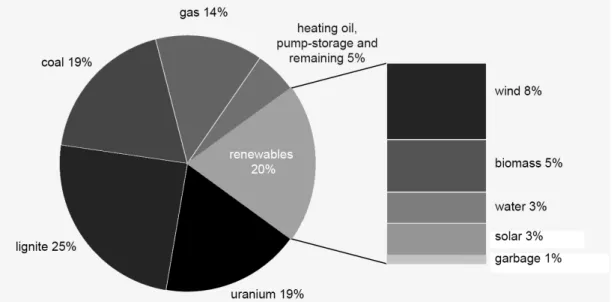
Figure 1: composition of German Power Generation 2011 ... 13
Figure 2: Merit Order of Power Plants ... 17
Figure 3: Spot Price EEX in the available dataset ... 19
Figure 4: Non-scheduled unavailability for nuclear power plants in MW ... 22
Figure 5: Comparison of Spot Prices, load and Feed-in of renewables ... 23
Figure 6: Correlogram of the spot price, full time horizon ... 26
Tables
Table 1: Summary Statistics for the 24 Spot Price Hours ... 20
Table 2: Summary statistics for the dataset ... 25
Table 3: Explanation of used variable names ... 42
Table 4: Estimation Results ARIMAX, ARIMA, MGARCH and OLS for hour 13 ... 43
Table 5: Forecasting Errors for September 2011 ... 48
Introduction 8
1
Introduction
As electricity markets become deregulated, the numbers of market participants at the power exchanges is increasing. To place reasonable bids, the participants have to build an own opinion about the future development of electricity prices at the spot market. There are several important factors which contribute to the settlement of electricity prices, for example the forecasted power consumption, the feed-in of renewable energies as requested by law, the price of input commodities like oil or emission certificates – and the unavailability of power plants. This thesis aims to work out the determinants of the electricity price and then use them to forecast electricity prices for the day-ahead electricity market. That way, the thesis also delivers an understanding for the importance of different variables for the electricity price. The data that will be used for this has to be published by the major utility companies due to an order of the regulation authority since about mid-2009. Since the data in question is rather new, this thesis is among the first scientific works making use of it in an econometric context.
The precise forecasting of electricity prices is of high importance for the market participants: First, market participants that own power plants have to adjust their bids to optimize the profit from their power plants. Second, market participants that have to buy electricity capacities need to decide whether on forward markets or at the spot market. Third, market participants are able to schedule the load of their power plants depending on the electricity prices that can be expected.
Following the modelling approach established by Box and Jenkins, the thesis develops a number of Time Series models, including an ARIMA, ARIMAX, MGARCH and an OLS model. The models will be estimated using two sub-samples of the available dataset. The explanatory power of the different models will then be discussed upon their prediction for a respective off-sample subset of the dataset.
Chapter 2 will introduce the specialities of electricity markets in general and show why the German electricity market is very relevant. The important determinants for the electricity price will be worked out. In Chapter 3, the availability of these variables will be checked and basic properties of the data will be explained. Chapter 4 starts with an overview of the available methodologies to model electricity prices and explain the chosen econometric models. Chapter 5 then presents the development of the models and the obtained results of the analysis. Chapter 6 concludes.
2
Determinants of the Electricity Price
2.1
Introduction on Energy Trading, European Power
Exchanges and Market Participants
As the aim of this work is to increase the understanding of electricity prices, this chapter will review the theoretic concepts of power markets in general and the German power market in particular and draw conclusions on the variables which are necessary to model electricity prices with econometric methods.
Today, electricity is a traded commodity but is different from other commodities like oil and gas in a number of aspects. The generation and consumption of electricity have to be balanced at all times to have a constant frequency in the grid. A continued imbalance of generation and consumption and the subsequent deviation from the grid’s target-frequency of 50Hz would end with the consequence of malfunction of electrical machines and blackouts. In addition, electricity can only be stored by means of converting it to another form of energy which comes at the cost of efficiency losses and in any case, these storage options are very limited. Because only one grid is economically feasible for a society, electricity transmission is a natural monopoly and needs to be controlled by regulatory authorities in order to enable fair market mechanisms.
During the process of liberalisation, power trading activities across Europe have risen considerably. Within Europe, Germany is the largest economy and power market in terms of electricity consumption. Germany’s annual power consumption 2010 amounted to about 590 TWh, with France taking the second place using about 510 TWh of electricity (RTE 2011; BMWi 2012). The four largest electricity producers RWE, E.ON, Vattenfall and EnBW hold a generation capacity of about 80% of the German market according to the federal competition authority (Bundeskartellamt 2011). The high voltage grids are also operated by only four transmission system operators (TSOs). The relevant power exchange for the spot market is the “EPEX Spot” which covers the markets Germany, France, Switzerland and Austria and is connected to the Belgian, Dutch and the Nordic market via market coupling mechanisms. The borders to Poland and the Czech Republic have explicit auctions (Tarjei 2011). The EPEX Spot has 211 members (EPEX SPOT 2011b), including the major power utilities of central Europe, transmission system operators, local energy companies and municipalities as well as pure energy trading companies and banks. Small
Determinants of the Electricity Price 10
companies which do not have direct access to the EPEX/EEX trading system can trade via separate accounts of other trading members. One main group of market participants are generators and retailers with intrinsic physical long or short positions, i.e. they have a certain customer base and a certain generation capacity and need to trade the difference on the power exchange. A second main group of market participants are pure traders and banks who typically aim to exploit prices differences to gain profit from arbitraging and take speculative positions.
Being the biggest power market in Europe, the large influence of renewable energies along with still large shares of conventional energy production and a diverse structure of market participants makes the German electricity market a very relevant one for an econometric analysis of power exchanges.
2.2
Power Generation and Demand Characteristics in
Germany
In this section, important determinants for the power price will be worked out for both the supply and the demand side of the market. Germany has a number of different technologies in use to generate electricity, each with different characteristics and dependencies towards the electricity price. Because of the balancing needs that have been described earlier, production is characterised by a mixture of heterogeneous types of power plants that have varying costs structures reflecting the need for flexibility. Base-load power plants usually operate for most of the time of the year and are characterised by high fixed costs and low marginal costs, while peak-load power plants are only used as needed and have comparatively low fixed costs but typically high marginal costs (Ockenfels et al. 2008).
Before going into the details of production, it is important to understand the concept of marginal costs in the context of electricity production. The marginal costs of electricity production include mainly the fuel costs and other variable costs of production. In addition to this, the marginal costs consist of the opportunity costs that arise if the production resources are not used in the manner with the highest possible value. As Ockenfels explains, occasionally the marginal costs cannot be defined clearly. For example, this can be the case if there are so-called “complementarities” or “non-convexities”, which are caused by start-up costs. Start-up costs are incurred upon every re-start of a power plant. These include costs for heating-up the power plant, network synchronisation and the increased wear and maintenance costs due to the temperature fluctuations (Ockenfels et al.
2008). These cannot always be calculated precisely and thus marginal costs cannot be defined clearly.
In the following, the different types of power plants in the German market will be presented as their properties are in turn an important determinant for the characteristics of the market. The most important power plants are those using rivers, wind and solar power, nuclear power, lignite and hard coal, gas and oil and finally pump storage power plants. When ordering power ascending order in terms of marginal costs, run-of-the-river power plants come first. These power plants are installed in large rivers like the Rhine River and make use of the constant water flow. They have very limited possibilities to store water and usually are operational around the clock as a typical base-load power plant. They have no fuel costs and little maintenance costs as they do not need constant supervision. These power plants can become unavailable in the event of low river levels or maintenance.
Second, there are wind and solar power plants. Due to little marginal costs, these power plants will also run whenever possible but as opposed to run-of-the-river power plants they have a much bigger variability in their power generation due to fluctuating wind and cloud coverage. The electricity companies employ meteorologists to predict wind speeds and insolation and therefore the generated power. The German law requires the power suppliers to feed the electricity generated by solar and wind power plants into the grid and they can be disconnected only in the case of emergencies for grid control. Therefore, wind and solar energy cannot be put into either the base- or peak-load category. Germany’s wind and solar capacities have grown considerably in the last years due to high feed-in tariffs, with jumps in capacity taking place prior to changes in these tariffs (Tarjei 2011).
Third, nuclear power plants generate electricity by the fission of radioactive molecules. Due to the high energy density of uranium they have little marginal costs once they are running, but it is considerably expensive and time-consuming to start and stop a nuclear power plant. However, it is possible to moderate the nuclear reaction by using the control rods and thereby control the power output to some extent. These characteristics make a nuclear power plant a typical base-load power plant. Unavailabilities can occur due to scheduled maintenances, which take about one month every year, low river-levels in summer and unscheduled shut downs out of security or political considerations.
Fourth, lignite and hard coal power plants facilitate coal combustion to generate electricity. Through the oxidation of coal, CO2 gets produced which by itself is a natural climate gas
Determinants of the Electricity Price 12
but contributes to the human-induced global warming due to the quantities humans exhaust of it currently. So called CO2-certificates are needed when one wants to run a coal power
plant in order to make its use less attractive and motivate reduction of CO2. Coal power
plants have less start-up and stop-costs than nuclear power plants but also need a couple of hours to reach full capacity. Modern coal power plants need less time than old ones as they are already designed for greater controllability needs. Also, coal power plants can be put into a standby-mode from which it can produce electricity on shorter notice than from a cold-start. Therefore, coal power plants have both base-load and to some extend peak-load usability. Unavailabilities can occur due to maintenance and also due to low river levels: Given low river levels, cooling might not be possible and ships might not be able to use the rivers for the transport of coal.
Fifth, gas power plants are considered very efficient power plants as they have a high efficiency-factor. They exhaust less CO2 than coal power plants for a given amount of
electricity but are considered more expensive than coal as per electricity produced, though prices have declined in the last years due to new discoveries in North America. They can start very quickly and therefore have good peak-load capabilities. Because gas is transported through pipelines, unavailabilities occur mostly due to maintenance. Transport interruptions of gas due to e.g. political decisions from Russia so far have not been an issue yet in Germany as there are plenty storage capabilities for gas from both tanks and the grid: Contrary to the electricity grid, the gas grid can be a storage in itself as one can increase the pressure of the gas. The gas price is often linked to the oil price in the long-term contracts between gas producers and the retailers, which was originally argued with the possibility of substitution between the two (Stern 2007). Oil power plants are similar in terms of usage to gas power plants but are only used in rare cases for peak-load purposes as oil is an expensive energy carrier and there are considerable CO2-emissions. Unavailabilities can occur for maintenances.
Sixth, there are pump storage power plants which do have a free energy source but that can come with considerable marginal costs: due to their superior possibilities of both producing electricity on very short notice within seconds and the possibility to pump water up into the basin, they can be sold as “Primary Reserve” in a separate market, the market for ancillary services, which is needed from TSOs for very short-term generation capabilities. Pump storage power plants are peak-load power plants and have little unavailabilities for maintenance. Other generation facilities like biomass or geothermal energy do not play a
significant role yet. With their unique ability to “store” generated electricity for later use, they have the ability to smoothen prices: Electricity is used to pump up water to the top basin during low prices and then used to generate power again when prices are high. The smoothing price effect of water power can be observed in Nord Pool’s electricity prices, which are less volatile than prices on the EPEX due to high capacities of water power plants. The total composition of energy sources for 2011 in Figure 1 shows, that energy production is still dominated by fossil fuels with lignite having a share of 25% of total production and coal and gas having 19% and 14% respectively.
Figure 1: composition of German Power Generation 2011, adapted from: BDEW (2012)
When shifting the focus from the supply side to the demand side of the electricity market, Bourbonnais and Méritet (2008) work out several factors on why electricity demand has characteristics that are different from most other commodities. Electricity demand is highly inelastic as it is a necessary product with very limited substitutes. In Addition, the demand is highly dependent on unforeseeable factors like climate and weather conditions. Also, electricity displays seasonal patterns due to economic activity and weather conditions. Seasonality can occur on various levels, including an hourly, daily, weekly, or monthly seasonality (Bourbonnais & Méritet 2008). Differences in electricity demand between countries can subsequently occur due to variations in climate and weather and also in the composition of electricity buyers, namely how much electricity is needed from households and from different kinds of industry. In Germany, temperature is less important for total demand compared to other countries due to the relatively large dependence on industrial
Determinants of the Electricity Price 14
activity of around 45% of total demand, the relatively little dependence on electricity for heating and few necessities for air conditioning (Tarjei 2011).
As a last important determinant of electricity prices, there are to mention congestion issues that can occur at national or regional borders. Congestion means the limited grid capacities between two adjacent networks. The more congestion issues there are, the more important issues about market power within a region will be and the electricity price will be higher. The less important congestion issues become, the lower the electricity price will be in areas that originally had a high price (Lise et al. 2008).
Through this analysis of the generation characteristics of the German electricity market, important variables for the price settlement could be determined: The composition of different base- and peak-load power plants, weather forecasts, the demand forecast, the amount of water power plants, interconnection capacities, planned and unplanned maintenance, the in-feed of renewable energies and the price of input commodities. These variables will be checked for availability and usability in the econometric analysis in Chapter 3.
2.3
Traded Products and Relevant Markets
For the purpose of this work, it is important to select the appropriate market and products for the econometric analysis. The two main marketplaces for day-ahead trading in Germany are represented by the power exchange EPEX Spot and electronic OTC trading.
Due to its liquidity and number of market participants, the EPEX Spot is the central trading point of the German day-ahead power market. Currently, the daily auction for the next day takes place at 12.00 pm, on each day of the weak including statutory holidays (EPEX SPOT 2011a). Liquidity on the Intraday Market, which covers the period after the day-ahead auction and the actual delivery period, is only a small fraction of the day-day-ahead auction and is only used for minor balancing purposes. Real time imbalances in the power system are balanced using generation units that can provide positive or negative primary, secondary and tertiary reserve energy under supervision of the TSOs. TSOs procure these types of reserve energy on separate markets (Johannes 2011).
Contrary to exchange-based trading, OTC trading takes places directly between the counterparties and is often facilitated by broker companies. The transactions are either executed via electronic broker platforms or bilaterally via telephone. According to
Johannes, most day-ahead trading activities take place between 8 a.m. and 12 p.m. on the day prior to the delivery day. Johannes points out that the continuous OTC market is important for market players to hedge larger volumes prior to the exchanged based auction at 12 p.m. Thus, the OTC-market can be considered to be the last forward market before the final EPEX Spot exchange clears (Johannes 2011). According to Tarjei, most of the trading volume of German power is in the OTC market. Similar to the trading on the exchange, spot contracts require physical delivery while the futures market can be physical or financial (2011). However, even though a large volume of the power trades are made via OTC and thereby independently from the systems of the power exchange, the price settlement through the power exchange will serve as a reference point, from which continued price data is available in a standardized form. This is why an econometric analysis should be based on EEX data and not on OTC data.
There is a range of spot price products with different hourly combinations that can be traded during the daily auction. Out of arbitrage considerations, the price of a product which includes a set of hours, e.g. a Base, Peak or Off-Peak contract, has to be equal to the sum of the individual hours. If this would not hold true, there would be riskless arbitrage opportunities for the market participants by shorting e.g. a high-priced product which has a combination of contracts, and closing the position again by buying the low-priced set of contracts. This “value additivity” not only holds true for the spot market, but also for the Futures market when one also considers the time value of money (Bjerksund et al. 2010). This means that by focusing on the individual hours for forecasting, the same conclusions can be drawn on the price of related products.
Besides the day-ahead and intraday markets which are linked to the physical delivery of electricity, there are derivatives markets which are purely financial and in which contracts on future deliveries are traded. These consist of futures contracts for weekly, monthly or yearly delivery usually up to three years in advance. Besides regular futures contracts, there is a wide range of other derivatives like e.g. European, American and Asian Options which are traded either on the EEX or OTC. Many energy suppliers use the derivatives market for hedging purposes and close open positions so as to limit risks and secure a certain profit margin – giving up possible higher prices in return. The percentage of power that is already hedged in advance is determined through the individual hedging, where conservative strategies involve hedging up to 100%.
Determinants of the Electricity Price 16
As Ockenfels et al. (2008) explain, even though a large part of the energy is traded in long-term contracts and only a comparatively small part is traded day-ahead in the spot market auctions, it is sensible to concentrate the econometric analysis on the spot market. This is due to the fact that the “prices in all upstream electricity markets actually reflect the expected spot market price” and hence it is the spot price that determines “the costs of electricity even in the long run”. This becomes even more compelling when considering the special conditions the spot price is subject to, as it is linked to the physical aspects of electricity while the derivatives are not linked to physical constraints considering their purely financial nature. Because of the lack of storability of electricity, power exchanges require comparatively complex rules and regulations along with a careful consideration of numerous ancillary technical conditions in the generation and transmission of electricity. Ockenfels et al. (2008) point out that the spot market auction complies with these demanding requirements.
2.4
Auction & Price mechanisms
In the auction, both bid prices for an individual hour and block bids comprising several contiguous hours can be submitted. The maximum admissible bid price has to be between -3,000 EUR/MWh and 3,000 EUR/MWh for all contracts. This wide range is used as the power exchange does not want to constraint price formation. Allowing negative prices is due to the possibility of negative marginal costs for some power plants in times of low demand. For instance, in a time of low demand like a Sunday, most power is generated by base-load power plants that run 24/7. For a limited time and in special cases, it might be cheaper for the owner of a nuclear power plant to increase power consumption by offering money to a consumer, rather than to shut down the nuclear power plant and lose all the profits for remaining time until it becomes operational again. In this case, the owner of the nuclear power plant is willing to pay a price to someone who can consume the energy. Negative Prices have been observed on various occasions in the past. In the dataset that will be used later on, 48 of 16,776 hours had prices below 0 EUR/MWh. The market participants making use of this opportunity will most likely be the owners of pump storage power plants, who will use the abundant power to pump up water into their storage basin.
The bids must be sent to EPEX Spot before 12PM on the day before delivery. Then, all bids are aggregated into supply and demand functions and converted into linearly interpolated sell or buy curves. The market price is established on the basis of the intersection of these supply and demand functions and thereby a market clearing price for
every hour of the following day is generated. Every market participant who supplies electricity during a given hour receives the respective price for that hour and every market participant who buys electricity during that hour pays that price. Since all participants have the same price, this mechanism is also referred to as the “uniform price auction”. In case the transmission capacity is not sufficient for the execution of the schedules determined in the auction, the market can be divided into price zones. However, this case has never occurred so far as the transmission system capacities within the trading area of EEX are currently sufficient compared to the quantities traded (Ockenfels et al. 2008).
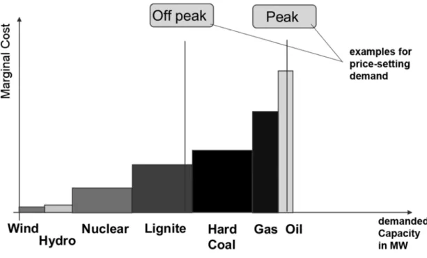
In theory and in practice, the resulting price is the marginal cost of the most expensive power plant from the group of least expensive power plants that are sufficient to cover the power demand. Figure 2 shows this “merit order”: power plants with the least marginal costs will be offered to the market at first because they will yield the highest profit. The rank of different technologies in the merit order can change as fuel prices change, i.e., gas and hard coal power plants may switch their respective ranks in the merit order when fuel prices change (Tarjei 2011).
Figure 2: Merit Order of Power Plants, adapted from Skrivarhaug (2010)
The merit order principle in theory allows for the possibility of exercising market power by withholding generation capacities, which is an issue widely discussed in public. By withholding a power plant, a market player with many other power plants can increase the profits of all other power plants on the market as the new settlement price increases
Determinants of the Electricity Price 18
(Ockenfels et al. 2008). That way, another aspect in modelling electricity prices can be the concentration of market power among certain market participants. Market power can be measured in numerical terms, e.g. through the use of the Lerner Index or the Concentration Index (Möst & Genoese 2009). Other works use a comparison of the marginal costs and the electricity price (Müsgens 2004). However, to be able to determine the influence of market power in an econometric setting, the time horizon of the dataset has to be sufficiently large to cover different magnitudes of market power. Such an analysis could e.g. be done by using data from the years of the regulated electricity market in which there were monopolies and ranging to the times of the deregulated energy market which supposedly will exhibit more competition. A cross-sectional analysis within a given point in time over different industries will not yield sufficient results for market power, as different industries exhibit idiosyncrasies so that comparative statistics will not reveal information about market power (Vassilopoulos 2003).
2.5
Role of Forecasts
As Weron and Misiorek elaborate, extreme price volatilities have forced the market participants of the electricity market to not only hedge against volume risks but also against price risks in the electricity market. Thus, opinions about future price movements formed through forecasting have become a crucial input in decision making and strategy development. This accelerated research in modelling and forecasting electricity prices with differences in the used methodologies and the used horizon. Weron & Misiorek distinguish between short-term, medium-term and long-term price forecasting (Rafał Weron & Misiorek 2006). The objectives of the three categories differ. While long-term forecasting is used for investment profitability analysis and planning, like determining future sites or fuel sources of power plants, medium-term or monthly time horizons are used for balance sheet calculations, risk management and derivatives pricing. Short term forecasts are e.g. used by a company that adjusts its production schedule depending on the forecasted hourly pool prices and its production costs and thereby maximizes profits. Accordingly, for spot markets the short term forecasts are of main importance (R. C. Garcia et al. 2005; Rafał Weron & Misiorek 2006). Every major market participants who takes part in the auction of the electricity price in one way or the other will need to form an opinion about the future development of the prices so as to be able to determine a reasonable bidding behaviour. Statkraft for example heavily bases its decisions for “Energy Management”, trading and hedging on the findings from the analysis and forecasting unit (Skrivarhaug 2010).
3
Data
In chapter two, the possible range of variables that have an influence on electricity prices have been worked out. Now, it is necessary to check these variables for availability for the public and to discuss their usability for econometric purposes. It will only be tried to obtain publicly available data. That way, it can be simulated what a 3rd party or a possible market entrant is capable of. Apparently, an existing electricity supplier will have superior data concerning its customer base than what is publicly available and thereby will be able to make more precise calculations on the electricity price.
3.1
Available Data
3.1.1
EEX: Spot Prices and CO2-Certificates
Figure 3: Spot Price EEX in the available dataset, 11 values below -50 EUR/MWh omitted
The spot prices are determined through the auctioning as described earlier and are available from EPEX on a per-hour basis, quoted in EUR/MWh. The data is available since 2002, which was the start of the EEX after the fusion of the power exchange Frankfurt and Leipzig. Since other relevant data is only available since November 2009, this work will start using data on spot prices from this date on. The available data reaches until the 30th September 2011 and accordingly includes nearly two years. This sample size is similar to earlier works as can be seen e.g. in the compilation of Aggarwal (2009). In the sample, the
-5 0 0 5 0 1 0 0 1 5 0 S p o tp ri c e i n E U R /M W h 11/2009 1/2010 6/2010 1/2011 6/2011 10/2011 Time
Data 20
price ranges between -199.99 EUR and 131.79 EUR and has a mean of 46.48 EUR. Peak-prices average at EUR 52.79 and off-peak Peak-prices at 40.16 EUR. Table 1 reveals considerable differences between the hours, especially the high values for the kurtosis in the morning hours will lead to interesting results in the forecasting performance.
Table 1: Summary Statistics for the 24 Spot Price Hours
The EEX also determines the price for CO2-certificates, which is done on each weekday since 2005. In the available dataset, the price has a mean of 14.24 EUR/t. For the use of this work, the price of Fridays has been assumed for Saturday and Sunday as CO2-certificates are not quoted on the weekend.
Electricity prices exhibit a phenomenon which is called spikes or more general: outliers. In some rare events, e.g. when cross-border capacity is remarkably low due to maintenance,
Hour Mean Std. Dev. Skewness Kurtosis
1 39.1 10.9 -4.9 67.3 2 35.4 12.0 -3.7 42.0 3 32.1 13.4 -3.1 28.7 4 29.5 15.1 -4.2 44.6 5 30.3 13.0 -2.6 27.4 6 34.2 12.8 -3.1 32.0 7 40.2 17.3 -4.6 56.3 8 48.6 19.1 -3.7 43.6 9 52.1 16.4 -2.1 20.0 10 53.8 13.1 -0.9 6.5 11 54.7 11.7 -0.5 4.1 12 56.1 11.3 -0.3 3.8 13 54.3 10.5 -0.4 3.7 14 51.5 11.5 -0.6 3.9 15 48.2 12.1 -0.6 4.2 16 47.5 12.0 -0.6 4.4 17 47.9 11.8 -0.4 5.0 18 53.4 13.7 1.0 7.8 19 56.9 12.2 0.8 6.2 20 55.9 10.7 0.3 3.2 21 52.5 9.7 0.1 2.9 22 48.6 8.3 0.1 3.2 23 48.6 7.4 -0.1 3.4 24 42.8 8.6 -2.4 21.3 all hours 46.48 15.2 -1.5 19.5
there is extraordinarily high wind in-feed or there are very low river levels, exceptionally high or low prices might occur. Some works filter the data by removing outliers, thereby reaching a smaller forecasting error. Since observations cannot be simply removed in a time series dataset, outliers can be filtered by capping the values at a certain threshold or using an average value instead of the outlier. Other works specifically focus on forecasting these exceptional events, like Christensen et al (2011) and Trueck (2007). In order to stay comparable with earlier works, ensure reproducibility and make the results more realistic, outliers have not been removed in the current analysis.
3.1.2
Transparency: Availability of Generation Capacity, Wind- and
Solar Feed-in
Due to European and national regulations, large power suppliers have to publish “market-relevant” information considering generation and consumption of electricity since 2009. The EEX publishes this data as a service for these companies on a central website after checking the data for plausibility, anonymizing it to some extent and aggregating it. Not all the owners of power plants have to publish this data, but about 91% of all generation capacity was available on this website at the time the data was downloaded (EEX 2011). In addition to being required by law to publish certain data, some power suppliers publish more data on a voluntary basis. The published data on the transparency website contains: the planned and unplanned unavailabilities of power plants, the planned and actual in-feed of solar/wind energy along with the planned and actual generation of conventional power plants.
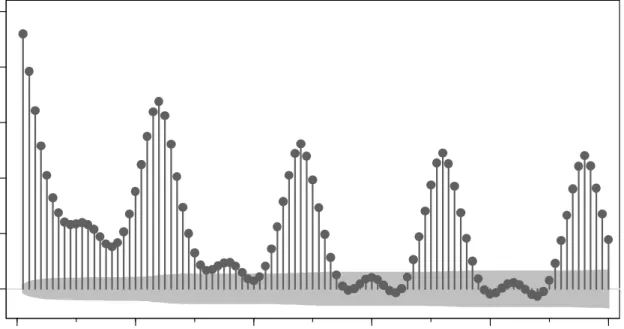
The planned unavailability of power plants can be e.g. scheduled maintenances, which are known up to several years in advance. Periods of unplanned unavailability can be due to emergency situations or low river levels that forces thermal power plants to shut down because of environmental concerns and regulations. An unavailability is stated as a time frame, e.g. the data set contains the information that 144 MW of a coal power plant within Germany is being unavailable between 4.11.09 18:00 until 9.11.09 5:00. To use the data in this work, the amount of unavailable power for the various types has been calculated for each individual hour of the dataset. In cases where unavailabilities are stated to start at some point within an hour, e.g. 18:25, the unavailability will be counted in the dataset from the next full hour, i.e. 19:00. As has been discussed, it will take some time for a power plant to start and stop operation in practice so the decline of power being generated will be rather smooth than sudden. As an example, the non-scheduled unavailabilities are shown
Data 22
for nuclear power for the whole data-sample in Figure 4, which includes the decision to shut down nuclear power plants in the aftermath of the Fukushima-catastrophe.
Figure 4: Non-scheduled unavailability for nuclear power plants in MW
The solar and wind in-feed is stated as induced power per each 15 minutes. To use the data in this work, the 4 quarters have been averaged to calculate the amount of MWh that is generated within one hour. The data for solar in-feed is not available until the 19th of July 2010 because the data has not been published on the transparency platform until that date and is noted as zero in the current dataset until that point in time.
As has been worked out in the preceding chapter, the expected demand in a given hour is an important variable in determining the electricity price. The total demand itself is not published on the transparency website. However, generation has to follow demand in an electricity grid and for that all the necessary information is given on the transparency website: There is the information about the total power generated from conventional power plants and the power generated from wind and solar is known as well. Not known are transmission and distribution losses, the power generated by smaller power producers that are not obliged to publish data on the transparency website, and small, decentralised power generation like industrial autogeneration, geothermal or block heat and power plants (Burger et al. 2007). However, this shouldn’t have major consequences for the price formation on the power exchange within the framework of a statistic model as it can be expected that the remaining demanded capacity should follow the same trends which the
0 2 0 0 0 4 0 0 0 6 0 0 0 U n a v a ila b ili ty U ra n iu m n o n -s c h e d u le d i n M W 11/2009 1/2010 6/2010 1/2011 6/2011 10/2011 Time
available data exhibits. Therefore, there are sufficient replacements for total power demand in the transparency data.
Figure 5: Comparison of Spot Prices, load and Feed-in of renewables
In total, the data published on the transparency website adds significant information that can be used for econometric analyses that has not been available for earlier works. Actually, many earlier works recommend to re-estimate their findings with exactly the data that has now been published on the transparency website, e.g. Swider & Weber (2007) and Garcia et al. (2005). Figure 5 shows an example of the explanatory power of this data: Periods of high wind are accompanied with drops in the generation of both conventional power and the spot price.
3.1.3
Remainder: Weather, Oil-Price, Transmission Capacity and River
Levels
As weather plays an important role in energy consumption, temperature is included in the dataset (e.g. Huurman et al. 2010). The data has been obtained from DWD, Deutscher Wetterdienst. Because the purpose of this work is to forecast day-ahead electricity prices, forecasts should have been obtained: However, due to availability reasons, only actual temperature data has been incorporated. That way, the implicit assumption is made that on average, the forecasted temperatures for the next day are exact. Weron & Misiorek (2008)
0 1 0 2 0 3 0 4 0 5 0 G e n e ra ti o n i n M W 0 2 0 4 0 6 0 8 0 S p o tp ri c e
Mon, 1.8. 0:00 Mon, 8.8. 0:00 Mon, 15.8. 0:00 Mon, 22.8. 0:00 Mon, 29.8. 0:00
Spotprice Planned Generation Quantity
Data 24
use the same assumption when they calculate an arithmetic average of big cities within the examined market to have a proxy for the average air temperature of the whole region. However, as only daily data for Frankfurt am Main was available for the use of this work, it has become the weather-data that is used as a proxy for the general temperature in Germany. Still, this produces significant estimates which will be shown later because Frankfurt is a rather central city.
In order to keep the number of variables that are used for the econometric analysis in a reasonable size, the oil price is used as a common proxy for the price of the input energy carriers like coal, gas, oil, and uranium. This seems reasonable due to the connection of oil and gas price through long-term contracts. For coal, there are many different prices depending on quality and origin and therefore there is no “one” price that can simply be added. According to Tarjei (2011), “Brent” is the relevant oil price for Germany as it is the crude oil blend from the North Sea. The oil price data is obtained from Thomson Reuters Datastream in USD per Barrel. Since the oil price is only listed for weekdays, the oil-price from Friday has been assumed to stay constant over the following weekend.
Another important issue for the determination of electricity prices can be congestion issues within the market or at its connections to other markets. Considering the auction of the electricity price, the internal transmission capacity has not yet lead to differences in pricing, even though the limited transmission capacity from Northern to Southern Germany has already led to various challenges for the TSOs. Transmission constraints are built into the auctioning system of EPEX Spot and there is the theoretic option of zonal prices but this has not yet occurred in the auction for the German electricity market. Accordingly, transmission constraints are not an issue right now for a statistical approach considering the forecasting of electricity prices but might be an issue in future in case wind production keeps increasing in northern Germany and the grid capacity cannot keep up with this increase. However, collecting the respective data will be difficult because congestions are not part of the transparency-system so far and the various congestion points differ in who manages them and whether they are part of the EPEX auction or auctioned separately.
As McDermott & Nilsen (2011) show, the river levels also have an influence on electricity prices. However, considering the sample size of about two years and the number of variables already included in this analysis, the river levels have not been obtained both due to availability and also to reduce risks of overspecification. As a proxy, temperature is
included as it is somewhat correlated with the river levels which are especially low in summer (McDermott & Nilsen 2011).
Table 2: Summary statistics for the dataset
In total, the dataset compromises 16,776 observations from the 1st of November 2009 to 30th September 2011 where each observation represents one hour and includes information about the spot price, the price for CO2-certificates, Crude Oil, temperature, planned wind and solar feed-in, the planned and unplanned non-availabilities for the different kinds of power plants and the total planned power generation for all other power plants that are part of the EEX transparency system. The resulting summary statistics are shown in Table 2.
Three hours in the dataset are affected by the changes to and from Daylight Saving Time. In order to have a complete dataset without any gaps, the mean of the hour before and the hour after has been used for values that are missing during these hours.
Variable Obs Mean Std. Dev. Min Max
Spotprice 16,776 46.5 15.2 -200.0 131.8
emissionprice 16,776 14.2 1.4 10.4 16.8
CrudeOilBrent 16,752 91.7 17.4 70.7 125.4
temperature 16,776 11.0 7.9 -12.2 28.5
non-usability planned lignite 16,776 1,915.3 1,220.8 0.0 5,916.0
non-usability planned gas 16,776 1,639.5 1,024.1 0.0 5,193.0
non-usability planned oil 16,776 230.9 239.3 0.0 1,658.0
non-usability planned pump-storage 16,776 537.0 442.2 0.0 2,320.4
non-usability planned coal 16,776 2,246.1 1,587.8 0.0 7,963.5
non-usability planned uranium 16,776 2,274.9 2,119.9 0.0 10,978.4
planned non-usability total 16,776 8,926.0 4,878.8 0.0 23,002.5
non-sched. non-usability lignite 16,776 1,148.1 713.0 0.0 4,684.0
non-sched. non-usability gas 16,776 486.2 415.8 0.0 2,334.0
non-sched. non-usability oil 16,776 13.9 74.5 0.0 772.0
non-sched. non-usability pump-storage 16,776 65.0 109.9 0.0 900.0
non-sched. non-usability coal 16,776 1,059.7 628.9 0.0 4,121.3
non-sched. non-usability uranium 16,776 1,077.6 1,647.1 0.0 6,220.1
non-sched. non-usability total 16,776 3,852.7 2,122.4 0.0 11,245.3
Planned Generation Capacity 16,776 44,667.4 8,342.1 20,714.0 67,666.2
Actual Generation Capacity 16,776 41,621.2 7,868.3 21,453.4 63,781.0
solar infeed plan 10,536 2,037.3 3,074.3 0.0 13,982.7
Data 26
3.2
Properties of the Electricity Spot Price
In this section, the most relevant of the available variables, the spot price data, will be examined for a number of statistical properties that are important for econometric time series modelling. Some of the variables like CO2- or oil-prices might exhibit special
properties as well but examining them as well apparently would be outside the scope of this work.
3.2.1
Autocorrelation
Autocorrelation is the correlation of a given variable with itself, most commonly with values earlier in time. This is an important feature of many time series compared to a cross sectional analysis as, at least in an economic context, a value will often depend on its earlier value and will not be randomly distributed.
Figure 6: Correlogram of the spot price, full time horizon
Autocorrelation can be visualised by using a correlogram which will plot the correlation of a variable given its lagged values as can be seen in Figure 6, which shows a plot of the full time series of the electricity prices against its own lagged values. Clearly, electricity prices have a strong autocorrelation towards the same hours of the former days, which is why the correlogram shows a peak at the marks at each 24 hours. All peaks lie outside the shaded area that represents the 95% confidence interval. There are also high correlations within the same day, which can be seen for the first lags. However, these correlations cannot be
0 .0 0 0 .2 0 0 .4 0 0 .6 0 0 .8 0 1 .0 0 A u to c o rr e la ti o n s o f S p o tp ri c e 0 20 40 60 80 100 Lag Bartlett's formula for MA(q) 95% confidence bands
used for the purpose of forecasting electricity prices as they won’t be known beforehand: All 24 hours of one day are auctioned simultaneously.
3.2.2
Stationarity
A time series exhibits stationarity, when the joint probability distribution remains stable over time and consequently also mean and variance do not change over time. A time series which does not have these characteristics is called non-stationary. The assumption of stationarity is needed for time series analysis because otherwise the relationship between two variables would change arbitrarily and one could not track correlations between the two in a regression analysis. Using non-stationary time series in a regression analysis can be risky as one might compute significant correlations even though there are none as both variables increase independently from each other. This is called a “Spurious Regression”. Non-stationarity is especially problematic in combination with highly persistent time series. A time series is highly persistent when it has a long memory towards even small shocks and therefore does not return to its former mean or variance, thereby becoming a non-stationary process (Verbeek 2008).
To test for stationarity and highly persistent time series, one can use a graphical analysis, a correlogram or the dickey fuller test. The dickey fuller test has the H0 that the time series has a unit root and therefore is non-stationary. This H0 is rejected at the 99% level for all 24 hours of the dataset when tested with the full time horizon, i.e. the time series does not exhibit non-stationarity in general. However, when examining periods of a shorter length of only about 50 days and for some off-peak hours in the dataset used for this thesis, stationarity can be a problem as the H0 of a dickey fuller test cannot always be rejected at high confidence levels. This could be the reason why some other authors explicitly examine issues connected with non stationarity on German electricity prices, as does Liebl (2010) for example
3.2.3
Heteroscedasticity
A sample exhibits heteroskedasticity, when the variance of the error term changes depending on the explanatory variables. When estimating the coefficient by the use of OLS, one has to use heteroskedasticity-robust standard errors so that the standard errors and, consequently, the t- and F-scores remain valid. The estimates of the coefficients however will remain unbiased also in the occurrence of heteroskedasticity (Wooldridge 2008).
Data 28
To test for heteroskedasticity, there are for example the White test, the Breusch-Pagan test or graphical tests. The White test basically consists of estimating the explanatory variables against the error term u as the explained variable. Should any of the explanatory variables turn out to be significant, one has to reject the H0 that the error term is homoscedastic. Using the OLS-regression that will be presented later in conjunction with a white test for the full time horizon, the H0 of homoscedasticity has to be rejected for every individual hour of the dataset at the 99% significance level besides hour 14, where the H0 is rejected with a 97% significance level according to the chi-square distribution. The Breusch-Pagan / Cook-Weisberg test for heteroskedasticity yields the same conclusion with a 99% significance for all hours. The difference in the significance level for the two tests could be due to the fact that the White test uses a relatively large number of regressors and therefore uses many degrees of freedom (White 1980; Wooldridge 2008).
The findings match with those of earlier works that describe electricity prices to exhibit a “nonconstant mean and variance” (R. C. Garcia et al. 2005) and significant heteroeskedasticity (Swider & Weber 2007).
4
Estimation Models and Methodology
4.1
Overview of available Models
Many different models are used in the literature to forecast electricity prices. Aggarwal et al. (2009) describe Game Theory models, Simulation models and Time Series models which are divided between parsimonious stochastic models, regression models and Artificial Intelligence models.
Game Theory Models try to model the strategies of the market participants and identify a solution of those games. A key point is the analysis of the strategic market equilibrium, which can be based on models like the Nash equilibrium, the Cournot model and others. As Game Theory Models require many assumptions, solutions can vary widely between different models (Haili Song et al. 2002; Cunningham et al. 2002; Aggarwal et al. 2009).
Simulation Models, also described as Fundamental Models, try to build an exact model of the system and the solution is found using algorithms that consider the physical phenomena the process is bound to. This mimics the actual dispatch with system operating requirements and constraints. As Tarjei (2011) explains, the supply and demand side of the electricity market are described and the price at which the two curves intersect is calculated. This price then “equals the marginal cost of the marginal power plant supplying power”. Fundamental models are used by utility companies as they have access to extensive datasets, e.g. Statkraft uses purely fundamental modelling in the spot market and forecasts the hourly dispatch for each of approximately 2500 modelled power plants in Europe (Skrivarhaug 2010). These models can provide detailed insights into the system prices though suffer two major drawbacks: First, they require detailed system operation data and second, the simulation methods are complicated to implement and the computational cost are very high. Furthermore, Simulation models make the assumption that a “fair” value will emerge, which can neglect market trends (Aggarwal et al. 2009).
Time Series analysis focuses on the past behaviour of the observed variable. There are models like multiple regression, autoregressive (AR), moving average (MA), autoregressive moving average (ARMA), autoregressive integrated moving average (ARIMA) and generalized autoregressive conditional heteroeskedasticity (GARCH) models. Normally these are univariate, i.e. focusing only on one variable and its passed values but can also be extended with exogenous variables, then being called multivariate
Estimation Models and Methodology 30
models. Besides these “parsimonious stochastic” time series models, there are also so called Artificial Intelligence models. According to Aggarwal et al. (2009), these nonparametric models “map input-output relationships without exploring the underlying process”. AI models are said to have the ability to learn complex and nonlinear relationships that are difficult to model with conventional methods. However, as Weron & Misiorek (2006) point out, these models are not intuitive and don’t have a simple physical interpretation attached which makes understanding the power market’s behaviour difficult.
An additional method to forecast spot prices is examined by Redl et al. (2009). In theory, when assuming an efficient market hypothesis, the forward price should be a reasonable indicator for the upcoming spot price. However, these approaches do not allow the development of an own opinion and can be influenced by speculations. Redl et al. find questionable results on the predictive power of forward prices as the trading strategies of the market participants actually seem to rely on the spot price: spot prices can be explained well by their own lagged prices whereas lagged forward prices do not significantly influence spot prices. The weak predictive abilities of futures are supported by findings from Hipòlit Torró (2007). Accordingly, one of the other methods described earlier is necessary to make an own forecast of spot prices possible.
For the purpose of this thesis, parsimonious time series models are the most suitable. Contrary to Game Theory Models, they need fewer assumptions because they can rely on more actual data and are therefore easier rooted to the examined circumstances. Yet, they do not need as much data as fundamental models which basically try to simulate the complete market conditions. Compared to Artificial Intelligence Models, the results of time series models will still be intuitive and accessible for interpretation. Drawbacks of Time Series Models are the reliance on past data for forecasting: Per definition it is not possible to forecast completely new market developments. In Addition, it is unlikely to precisely forecast extreme events, as a forecast based on past data will have a tendency towards the mean. These two issues might be tackled by sophisticated fundamental models.
Thus, a number of stochastic time series models will be used for this analysis and discussed in more detail in the following. The most common approaches for time series modelling of electricity prices are a multiple regression using Ordinary Least Squares, and autoregressive moving average models along with conditional heteroskedasticity models using Maximum Likelihood estimation.
4.2
Time Series
4.2.1
Multiple regression and Ordinary Least Squares
The most common method to analyse time series is a multiple regression analysis and using “Ordinary Least Squares” (OLS) to estimate the coefficients. OLS computes the coefficients by minimizing the squared residuals between the observations and a fitted line. In the following, a “multiple regression” is always meant to be estimated with OLS.
The Gauss-Markov Assumptions for time series regressions, which need to be met for a multiple regression OLS analysis, are: First, that the stochastic process follows the linear model
= + + ⋯ + + ,
where y is the explained variable for time period t, are the coefficients of the explanatory variables and is the error term for t. Furthermore, the assumptions require that there is no perfect collinearity and that the error term u has an expected value of zero for any value of the explanatory variable in any given time period. If these first three assumptions hold, it can be shown that the OLS estimators are unbiased (Wooldridge 2008). Additionally, if the variance of the error term u is the same for all time periods and does not depend on any of the explanatory variables and the errors of two different time periods are uncorrelated for all explanatory variables, the OLS estimators can be shown to are “BLUE", the best linear unbiased estimators depended on the explanatory variables (Wooldridge 2008).
Electricity prices exhibit heteroscedasticity. This means that even though the estimation of the coefficients will still be correct, the standard errors and therefore the t-statistics will be biased. This will be corrected by using “robust” standard errors.
4.2.2
ARMAX and Maximum Likelihood
Many works in the field of forecasting day-ahead electricity prices with econometric methods rely on special time series models like ARMA which will be explained in this chapter and GARCH, which will be explained in the next. ARMAX is a special time series model that includes both an autoregressive term (“AR”), a moving average term (“MA”) and additional exogenous variables (“X”). While the nature of autoregression has already been explained in Chapter 3.2., it is necessary to point out what the notion of a moving
Estimation Models and Methodology 32
average is about: While autoregression captures correlations of the dependent variable with its own former values, the moving average component of the ARMAX model captures past deviations or shocks of the dependent variable and its own lagged values. These could be e.g. due to trends, a seasonality, or variables which are captured by neither the autoregressive term nor the exogenous variables. Thus, the moving average term is useful in describing time series in which events have an immediate effect that only lasts a short period of time (Wei 1990). Another addition that can be done in this context is the differencing of adjacent observations, which is helpful to in order to cope with stationarity issues. Then, the incremental development of the data is observed instead of the absolute values. In this case, the model is called an ARIMA model, the “I” standing for “integrated”, because after the estimation of the models the data needs to be integrated to reverse the initial differencing.
An ARMA approach differs from a “standard” multiple regression in two ways: While an AR term still can be explicitly modelled in a multiple regression analysis, the moving average term cannot. In addition, the estimation of the coefficients is not done using ordinary least squares but rather a maximum likelihood routine, because a non-linear fitting procedure is necessary. The reliance on ARMA and related models by the existing time series literature is believed to be also partly due to historic reasons; when autocorrelation was considered a nuisance when it was not modelled explicitly in the OLS model and that way standard errors were wrong and the estimates no longer efficient (Golder 2007).
When looking at a more formal definition, there are disturbances which are defined to be the error after fitting and can be calculated through = − where is the predicted and the actual price at time step t. The ARMA model is based on the assumption that the error term follows a white noise process, generally assumed to be normally distributed with the form = . . . , . The time invariant parameters mean and standard deviation can be estimated by maximizing the log-likelihood function. In the ARMA(p, q) model the relation between the observations and the disturbances is given by
(Swider & Weber 2007). The model is based on considering previous values of the process as a combination of an autoregressive (AR) and a moving-average (MA) part, where the AR part has the order p and the MA part the order q. In this notation, p is referring to the number of previous values of and q is referring to the number of previous values of the disturbances . The ARMA(p, q) model may then be extended by additional consideration of exogenous variables , with which the model then can be described as
= + = ∝ + + ! , "
+
where r describes the number of exogenous variables and the model can then be referred to as ARMAX(p, q, r). The parameters ∝ , and ! can then be estimated by maximizing the log-likelihood function (Swider & Weber 2007).
As Enders explains, the Maximum Likelihood (ML) estimation uses the following principle: If values of { } are drawn from a normal distribution with a mean of zero and a constant variance ², from standard distribution theory the likelihood & of any realisation of would be
& = ' 1
)2+ ², - . ' −
2 ²,.
As the realisations are independent from each other, the joint realisation for all values of t is the product of the individual likelihoods. Hence, given the same variance for all
realisations, the likelihood for the joint realisation is
& = / ' 1 )2+ ², - . ' − 2 ², 0 .
The method used in maximum-likelihood estimation is to select the distributional parameters so as to maximize the probability of drawing the observed sample (Enders 2010). As a simple example, could be generated from the model
= −
Accordingly, maximizing the log-likelihood function would involve solving for the values for and .
Estimation Models and Methodology 34
Literature is not clear if one has to correct for heteroscedasticity to get correct test statistics, so as a precaution, robust standard errors will be used in the following when estimating the models. Earlier works that forecast electricity prices using ARMA techniques usually did not state explicitly that robust standard errors are used. Even though this does not influence the outcome of the forecasts, it can be a factor in the development of the forecasting models, when the significance of the coefficients needs to be evaluated.
4.2.3
GARCH and Maximum Likelihood
Electricity prices have the special property that large price changes are often again followed by large price changes. For example, in the case of little demand and large wind in feed, prices will fall abruptly but when this special situation is gone, prices will change by a similar magnitude to the original level again (“Mean Reversion”).
By applying a GARCH approach, this conditional heteroscedasticity can be considered. Conditional heteroscedasticity means a time variant variance t in which large changes tend to follow large changes, and small changes tend to follow small changes, which is described as the volatility clustering. GARCH(p, q) models are designed to capture this changing volatility by calculating the variance in the following way:
= 1 + ∝ +
Accordingly, the time variant variance is described with a constant part ω, an AR-part of order p and a generalized MA-part of order q. A necessary condition is that the variance is positive at any time step t, i.e. that 1 > 0, 4 ≥ 06 and ≥ 0. The GARCH term will be included in a regular ARIMA model to model the white noise and the parameters can then be estimated by maximizing the log-likelihood function. As the name indicates, GARCH is a more generalized version of the ARCH model for which Robert F. Engle received the Nobel Prize in Economics 2003. In the ARCH model, the volatility is only depended on the realisation of the error term in the previous period(s) and not also on its own realisation in the previous period(s). Accordingly, a GARCH(0,1) model is the same as an ARCH(1) model. A GARCH model that makes use of exogenous variables is called an MGARCH. In the estimation of the GARCH model, no heteroskedasticity-robust standard errors will be used as the model explicitly models the variance (Swider & Weber 2007; Enders 2010).