Statistical Machine Learning Methods for High-dimensional Neural Population Data Analysis

High-dimensional Neural Population Data

Analysis

Yuanjun Gao

Submitted in partial fulfillment of the requirements for the degree

of Doctor of Philosophy

in the Graduate School of Arts and Sciences

COLUMBIA UNIVERSITY

Yuanjun Gao All Rights Reserved

Statistical Machine Learning Methods for High-dimensional Neural Population Data Analysis

Yuanjun Gao

Advances in techniques have been producing increasingly complex neural record-ings, posing significant challenges for data analysis. This thesis discusses novel sta-tistical methods for analyzing high-dimensional neural data. Part one discusses two extensions of state space models tailored to neural data analysis. First, we propose using a flexible count data distribution family in the observation model to faithfully capture over-dispersion and under-dispersion of the neural observations. Second, we incorporate nonlinear observation models into state space models to improve the flex-ibility of the model and get a more concise representation of the data. For both extensions, novel variational inference techniques are developed for model fitting, and simulated and real experiments show the advantages of our extensions. Part two dis-cusses a fast region of interest (ROI) detection method for large-scale calcium imaging data based on structured matrix factorization. Part three discusses a method for sam-pling from a maximum entropy distribution with complicated constraints, which is useful for hypothesis testing for neural data analysis and many other applications related to maximum entropy formulation. We conclude the thesis with discussions and future works.

List of Figures iv

List of Tables viii

1 Introduction 1

1.1 Neuroscience and statistics . . . 2

1.2 Dimensionality reduction for neural data . . . 3

1.3 Latent variable models and state space models . . . 5

1.4 Statistical inference for latent variable models . . . 7

1.5 Overview of the thesis . . . 14

I

Neural Population Data Analysis with Latent Variable

Models

16

2.2 Generalized count distributions . . . 20

2.3 Generalized count linear dynamical system model formulation . . . . 23

2.4 Inference and learning in GCLDS . . . 25

2.4.1 E-step: variational inference with dual optimization . . . 26

2.4.3 Practical concerns . . . 29

2.4.4 Dual optimization for E-step . . . 30

2.5 Model evaluation by leave-one-neuron-out error . . . 34

2.6 Experiments . . . 35

2.6.1 Simulation examples . . . 35

2.6.2 Real data analysis . . . 36

2.7 Discussion . . . 41

3 Linear Dynamical Neural Population Models Through Nonlinear Embeddings 43 3.1 Introduction . . . 44

3.2 Notation and overview of neural data . . . 45

3.3 Latent LDS neural population models with a linear rate function . . . 46

3.4 Nonlinear latent variable models for neural populations . . . 48

3.5 Inference by Auto-encoding variational Bayes . . . 49

3.6 Experiments . . . 53

3.6.1 Simulation examples . . . 54

3.6.2 Real data analysis . . . 57

3.7 Discussion . . . 62

II

Region of Interest Detection for Calcium Imaging Data 64

4.2 Algorithm . . . 68

4.2.1 Problem formulation . . . 68 ii

4.2.3 Shape fine-tuning . . . 72

4.2.4 Other details . . . 74

4.3 Experiments . . . 75

4.3.1 Simulation examples . . . 75

4.3.2 Real data analysis . . . 76

4.4 Discussion . . . 80

III

Maximum Entropy Flow Networks

81

5.2 Background . . . 86

5.2.1 Maximum entropy modeling and Gibbs distribution . . . 86

5.2.2 Normalizing flows . . . 87

5.3 Maximum entropy flow network (MEFN) algorithm . . . 88

5.3.1 Formulation . . . 88

5.3.2 Algorithm . . . 89

5.4 Experiments . . . 91

5.4.1 A maximum entropy problem with known solution . . . 91

5.4.2 Risk-neutral asset pricing . . . 94

5.4.3 Modeling images of textures . . . 97

5.5 Discussion . . . 102

6 Conclusion and discussion 104

Bibliography 107

1.1 Graphical model representation of state space model . . . 6 2.1 Left panel: mean firing rate and variance of neurons in primate

mo-tor cortex during the peri-movement period of a reaching experiment (see §2.6.2). The data exhibit under-dispersion, especially for high firing-rate neurons. The two marked neurons will be analyzed in detail in Figure 2.2. Right panel: the expectation and variance of the GC distribution with different choices of the function g . . . 22 2.2 Examples of fitting result for selected high-firing neurons. Each row

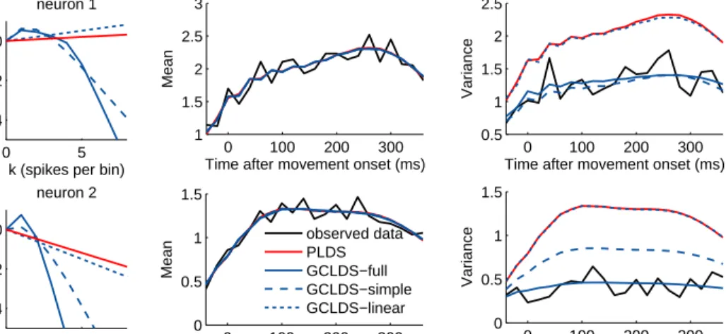
corresponds to one neuron as marked in left panel of Figure 2.1 – left column: fittedg(·)using GCLDS and PLDS;middle and right column: fitted mean and variance of PLDS and GCLDS. See text for details. . 38 2.3 Goodness-of-fit for monkey data during the reaching period –left panel:

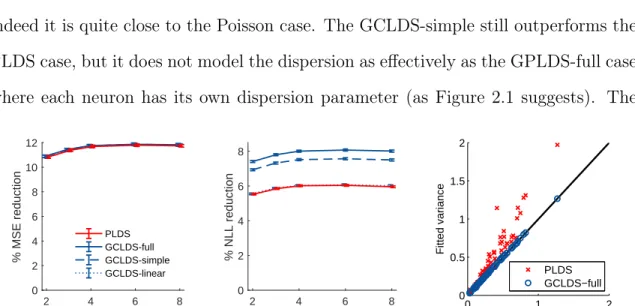
percentage reduction of mean-squared-error (MSE) compared to the baseline (homogeneous Poisson process); middle panel: percentage re-duction of predictive negative log likelihood (NLL) compared to the baseline; right panel: fitted variance of PLDS and GCLDS for all neu-rons compared to the observed data. Each point gives the observed and fitted variance of a single neuron, averaged across time. . . 39

panel: Temporal cross-covariance averaged over all81units during the preparatory period, compared to the fitted cross-covariance by PLDS and GCLDS-full. Right panel: fitted variance of PLDS and GCLDS-full for all neurons compared to the observed data (averaged across time). . . 41 3.1 Sample simulation result with “grid cell” type response. Left panel:

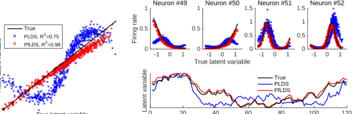
Fitted latent variable compared to true latent variable; Upper right panel: Fitted rate compared to the true rate for 4 sample neurons;

Bottom right panel: Inferred trace of the latent variable compared to true latent trace. Note that the latent trajectory for a 1-dimensional latent variable is identifiable up to multiplicative constant, here we scale the latent variables to lie between 0 and 1. . . 57 3.2 Results for fits to Macaque V1 data (single orientation) (a)

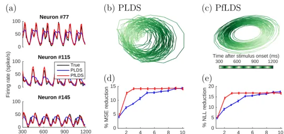
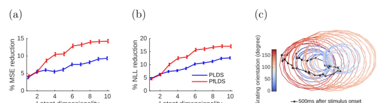
Compar-ing true firCompar-ing rate (black line) with fitted rate from PLDS (blue) and PfLDS (red) with2 dimensional latent space for selected neurons (ori-entation 0◦, averaged across all 120 training trials); (b)(c) 2D latent-space embeddings of 10 sample training trials, color denotes phase of the grating stimulus (orientation 0◦); (d)(e) Predictive mean square error (MSE) and predictive negative log likelihood (NLL) reduction with one-step-ahead prediction, compared to a baseline model (homo-geneous Poisson process). Results are averaged across 12orientations.

. . . 59

NLL reduction. (c) 3D embedding of the mean latent trajectory of the neuron activity during 300ms to500ms after stimulus onset across grating orientations 0◦,5◦, ...,175◦, here we use PfLDS with 4 latent dimensions and then project the result on the first 3 principal compo-nents. . . 60 3.4 Macaque center-out reaching data analysis: (a) 5sample reaching

tra-jectory for each of the 14 target locations. Directions are coded by different color, and distances are coded by different marker size; (b)(c) 2D embeddings of neuron activity extracted by PLDS and PfLDS, circles represent 50ms before movement onset and triangles represent 340ms after movement onset. Here 5 training reaches for each tar-get location are plotted; (d) Predictive negative log likelihood (NLL) reduction with one-step-ahead prediction. . . 61 4.1 Simulated calcium data. . . 77 4.2 Real calcium data. . . 78 4.3 ROI detection for the full Misha data, each sub-figure represents a z-slice. 79

truth. Left panel: The normal densityp0(purple) and iid samples from p0 (red points). Middle panel: The MEFN transformsp0 to the desired

maximum entropy distribution pφ∗ on the simplex (calculated density

pφ∗ in purple). Truly iid samples are easily drawn fromp_φ∗ (red points)

by drawing from p0 and mapping those points through fφ∗. Shown in

the middle panel are the same points in the top left panel mapped through fφ∗. Samples corresponding to training the same network as

MEFN to simply match the specified moments (ignoring entropy) are also shown (dark green points; see text). Right panel: The ground truth (in this example, known to be Dirichlet) distribution in purple, and iid samples from it in red. . . 93 5.2 Constructing risk-neutral measure from observed option price. Left

panel: fitted risk-neutral measure by Gibbs and MEFN method. Mid-dle panel: Q-Q plot for the quantiles from the distributions on the left panel. Right panel: observed and fitted option price for different strikes. 96 5.3 Analysis of texture synthesis experiment. See text for description. . . 99 5.4 Random samples (first 5 columns) and the mean image of 20random

samples (last column) from texture net (upper row) and MEFN (bot-tom row) for the stone example. . . 100 5.5 Brick example result. First row gives the raw input. The bottom 3

rows give 5 random samples (first 5 columns) and the mean image of 20random samples (last column) from texture net (row 2) and MEFN with large initial texture cost penalty (row3) and smaller initial texture cost penalty (bottom row) for the brick example. . . 101

2.1 Special cases of GCGLM. For all models, the GCGLM parametrization for θ is only associated with the slope θ(x) = βx, and the intercept

α is absorbed into the g(·) function. In all cases we have g(k) = −∞ outside the stated support of the distribution. Whenever unspecified, the support of the distribution and the domain of theg(·)function are non-negative integers _N. . . 24 2.2 Simulation result for PLDS and GCLDS. Showing the

leave-one-neuron-out mean square error (MSE) and negative log likelihood (NLL) for PLDS and GCLDS, as well as the improvement of GCLDS over PLDS. Results are averaged across50independent repeats with standard error showing in parentheses. . . 37 3.1 Simulation results with a linear observation model: Each column

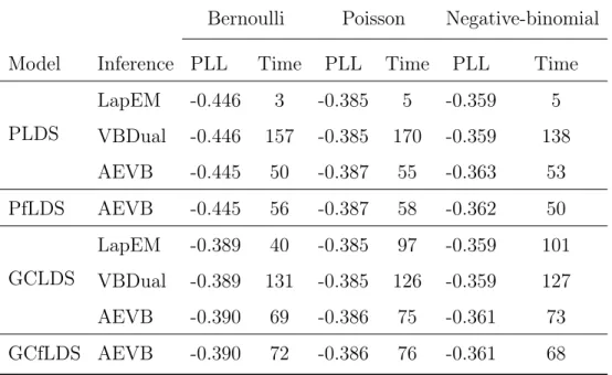
con-tains results for a distinct experiment. For each generative model and inference algorithm (one per row), we report the one-step-ahead pre-dictive log likelihood (PLL) and computation time (in minutes) of the model fit to each dataset. . . 56 5.1 Quantitative measure of image diversity using 20 randomly sampled

images . . . 100

Five years ago, when I first arrived at New York, I expected that the following few years can be tough. What I did not expect is how this five years would expand my mind so much and make me such a different person. This thesis would be impossible without the support and help of many people from Columbia statistics department, my friends and my family.

First I would like to thank my committee members. My academic advisor Dr. John Cunningham, who is organized, energetic, supportive and caring, provided me with valuable guidance and insights. It is his constant encouragement that makes me productive enough to finish several nice projects during my Ph.D. study. Dr. Liam Paninski aroused my interest in computational neuroscience by showing fascinating animations of decoding the primate motor cortex in a student seminar. I explored many interesting projects with him and was constantly amazed by his knowledge and depth of thinking. Dr. Tian Zheng was my mentor in my first year of PhD study. She gave me confidence in studying and researching, developed my interest in applied statistics and introduced me to many interesting research areas. I would also like to thank Drs. John Paisley and Mark Churchland for being in my committee and for careful reading of my thesis manuscript.

During my study in Columbia, I had the opportunity to participate a few other interesting research projects which I was not able to put in this thesis. I thank Drs. Andrew Gelman, Rahul Mazumder, Matthew Connelly, Shawn Simpson and Lauren

my skills significantly.

I was very lucky to be in an active research group. I would like to thank Evan Archer, Daniel Soudry, Josh Merel, Eftychios Pnevmatikakis, Ari Pakman, Uygar Sumbul, Gabriel Loaiza-Ganem, Lars Buesing, Xuexin Wei, Christian Andersson Naesseth, Scott Linderman and David Pfau, among others, for the helpful discus-sion and collaboration. I appreciate the opportunities to learn from them.

I would like to thank many researchers for providing data for the the research. Krishna V. Shenoy, Byron Yu, Gopal Santhanam and Stephen Ryu provided the macaque motor cortical data. Arnulf Graf, Adam Kohn, Tony Movshon, and Mehrdad Jazayeri provided the macaque V1 data. Misha Ahrens provided the zebrafish data.

I would like to thank my friends Shuaiwen Wang, Haolei Weng, Yuting Ma, Lu Meng, Jingjing Zou, Lisha Qiu, Yixin Wang, Yilong Zhang, Qiao Feng, Tianchen Qian, Guohui Guan, Tiantian Nie, Liang Liang, Mingsi Long, Xufei Wang, Shiman Ding and Yinting Hu, among others, for cheering me up when I was down, and for the helpful and enlightening discussions about both research and life.

Finally I would like to thank my parents, Ying Li and Zhi Gao, who made me a smart and hard-working kid and constantly supported me during my Ph.D. study. I owe so much to them for their love and support.

Chapter 1

Introduction

Until recently, neural data analysis techniques focused primarily on the analysis of single neurons and small populations. However, new experimental techniques have enabled the simultaneous recording of ever-larger neural populations [Robinsonet al., 2012; Ahrens and Keller, 2013; Prevedelet al., 2014]. The abundance of data provides both opportunities and challenges for neural data analysis, and has spurred a search for new statistical methods [Stevenson and Kording, 2011; Cunningham and Yu, 2014; Gao and Ganguli, 2015] . Indeed, statistical models have provided principled ways to performing signal processing, exploratory analysis, statistical modeling, scientific hypothesis testing, etc. This thesis introduces a set of methods related to high-dimensional neural data analysis.

The rest of this chapter provides high level motivation and background for the thesis, and provides an overview for the rest of the thesis.

1.1

Neuroscience and statistics

Neurons communicate by generating temporally fast (∼1ms) electrical signals called action potentials, or “spikes”. The temporal sequence of action potentials generated by a single neuron is called its “spike train”, which can be represented by a one-dimensional point process. The spike trains encode external stimuli and intentions, allowing humans or animals to understand complex environments and perform com-plicated tasks. Understanding how the billions of neurons in the brain respond to external stimulus, process and transmit information, and control the behavior is an important question. And statistics has been playing a significant role in the neu-roscience community in many aspects [Kass et al., 2005; Paninski et al., 2007]. We give a brief overview for the main contributions of statistical methods in neuroscience below.

To begin with, converting noisy observations from various neural recording tech-niques into clean signal requires specific statistical models. For electrophysiological data, clustering, mixture models and factor analysis techniques have been extensively applied to the detection and classification of spikes from recorded voltage signals, also known as “spike sorting”. See Lewicki [1998] for a review. For calcium imaging data, many statistical methods exist for region of interest detection and calcium de-convolution [Mukamelet al., 2009; Vogelsteinet al., 2009; Pnevmatikakiset al., 2016; Friedrich and Paninski, 2016].

Many statistical methods are also highly needed for exploring and understanding the structure of the neural data. Early attempts include using summary statistics such as peristimulus time histogram (PSTH) [Gerstein and Kiang, 1960] and spike triggered average [de Boer and Kuyper, 1968; Theunissen et al., 2001] to visualize single neuron activities given certain stimuli. Supervised learning techniques such as

generalized linear models (GLM) [Paninski, 2004; Truccolo et al., 2005; Stevensonet al., 2008] provide statistical formulations that link the spiking data to stimuli, spik-ing history and interneuron interactions. Unsupervised learnspik-ing techniques such as principle component analysis (PCA) [Churchlandet al., 2012] and state space models [Lawhernet al., 2010; Mackeet al., 2011] provide useful data tools for visualizing and understanding high-dimensional neural data.

Scientific hypotheses of neural data are formulated and tested under statistical frameworks, providing better understanding of the neural data structure [Olshausen and Field, 1997; Schneidman et al., 2006; Churchland et al., 2012]. Applications such as neural prosthetics [Shenoyet al., 2011; Gilja et al., 2012] and optimal exper-iment design [Nelken et al., 1994; Lewi et al., 2011] have also benefited greatly from statistical methods.

Recent developments in technology enabled simultaneous recordings of neuron populations, which can be represented as a high-dimensional time series. Statistical methods that capturing the key structure of the high-dimensional neural activities allow better understanding of the underlying mechanism of neural activities and are becoming more important in computational neuroscience [Cunningham and Yu, 2014]. Below we introduce dimensionality reduction techniques.

1.2

Dimensionality reduction for neural data

Many studies and theories in neuroscience posit that high-dimensional neural spike trains are a noisy observation of some underlying, low-dimensional, and time-varying signal of interest. A line of research has focused on developing dimensionality re-duction techniques for neural data that captures the key structure of the data. As discussed in Cunningham and Yu [2014], dimensionality reduction techniques enable

better data visualization for the neural activity, facilitate single trial data analysis, and shed light on the structure of neural population response.

DenoteX ∈_RT×n _{as then-dimensional data withT observations. Dimensionality}

reduction methods aim to identify a reduced version of the dataZ ∈_RT×m _(mn)

that captures the key features of the data. Linear dimensionality reduction methods, such as principal component analysis (PCA) and factor analysis (FA), in general takes the form of matrix factorization, where we aim at approximating the data by a low rank matrix

X ≈Z·C, (1.1)

where C ∈ _Rm×n _{links the reduced data to the full data. Nonlinear dimensionality}

reduction methods usually try to identify a nonlinear mapping that relates the reduced dataZwith the full dataX[Roweis and Saul, 2000; Tenenbaumet al., 2000; Lawrence, 2004].

In the spike train setting,Xrepresents (maybe a transformed or smoothed version of) the spike counts of n neurons in T time bins. Matrix Z represents a learnt low-dimensional latent intensity that captures the main variability of the data and can be used to provide visualization for neuron activities. Matrix C describes how the low-dimensional intensity is linked to the observation and can be used to summarize the behavior of each neuron. In calcium imaging setting, X represents the n-dimensional vectorized image recorded inT time bins, which can be decomposed as a product of spatial componentsZ representing shape of neurons (or other regions of interest) and temporal components C representing the activity of each neuron.

Building low-dimensional models for neural spike train data setting is complicated by the discrete observation and the temporal structure. The spike count data does not conform to the commonly used Gaussian assumption and requires count

distribu-tion families (Poisson distribudistribu-tion, for example) to describe its distribudistribu-tion [Paninski, 2004; Truccolo et al., 2005; Macke et al., 2011; Pfau et al., 2013]. The spike train also exhibits rich temporal dynamics, and incorporating the temporal structure in the model can help de-noise the data and more faithfully capture the structure [Yuet al., 2009; Mackeet al., 2011]. Among the various formulations for dimensionality reduc-tion, state space models, or more generally latent variable models, provide a popular framework for neural data modeling due to its generative nature and flexibility. We briefly introduce the main idea of this framework in the next section.

1.3

Latent variable models and state space models

Latent variable models are a class of probabilistic models that models the generative process of the observation by hidden variables that are linked to the observation. La-tent variable modeling provides a natural and principled way of modeling the structure of the data that are affected by unseen hidden variables, and is useful for summarizing the data, handling missing data, making predictions and so on.

Formally, latent variable models assume that the observation x is affected by unobserved variablesz and propose a probability distribution familypθ(x,z)

param-eterized by parameterθ. Model fitting involves identifying optimal model parameters

θ as well as the latent variables z, both of which are of interest in data analysis. Latent variable modeling is natural in neural data analysis since the observed neu-ral activities are highly coupled with unobserved neurons, intention, behavior and external stimuli [Sahani, 1999; Kulkarni and Paninski, 2007; Mackeet al., 2011].

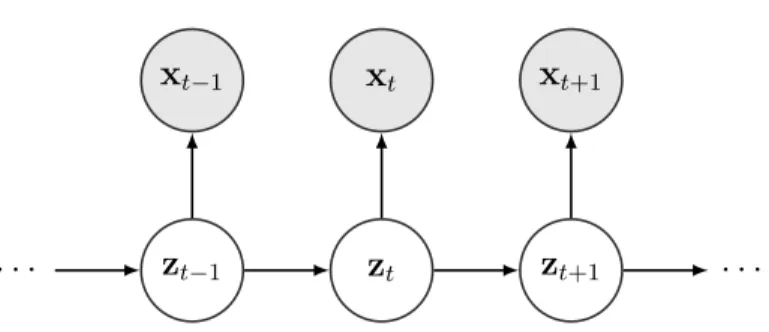
State space model is a class of latent variable models that models time series data x = {x1, ...,xT} (xt ∈ Rn for t = 1, ..., T) by assuming a hidden time series

zt−1 zt zt+1

xt−1 xt xt+1

· · · ·

Figure 1.1: Graphical model representation of state space model coupled with the observation. The generative model is specified by

• initial latent state distribution: p(z1),

• dynamic model specifying the evolution of the latent states: p(zt+1|zt) for t =

1, ..., T −1,

• observation modelp(xt|zt) fort = 1, ..., T.

Figure 1.1 gives the graphical model representation of state space models. The joint distribution is therefore of the form

p(x,z) = p(z1) T−1 Y t=1 p(zt+1|zt) T Y t=1 p(xt|zt). (1.2)

The latent variables encode a rich dependency structure through both the dynamic model and the observation model. And the Markovian structure of the latent variable helps make the model interpretable and the inference tractable (in certain cases). Those advantages lead to natural applications of state space model in neural data [Brownet al., 2001; Paninskiet al., 2010; Mackeet al., 2011]. The model is especially related to the dynamical view of the motor cortex, which states that neural activities in motor system reflect both the outputs to drive the motion and the internal processes that helps to generate motion but is poorly described by the motion [Churchland et al., 2012; Shenoy et al., 2013]. This dynamical system view has been essential for

building robust algorithms for neural prosthetics [Shenoy et al., 2011; Gilja et al., 2012; Kao et al., 2015]

The most commonly used state space model assumes a linear Gaussian structure,

p(z1)∼N(µ1, Q1), (1.3) p(zt+1|zt)∼N(Azt, Q), (1.4)

p(xt|zt)∼N(Czt,Σ), (1.5)

where µ1 ∈ Rm and Q1 ∈ Rm×m give the expectation and covariance of the initial

states,A∈_Rm×m _{models the relation of the states of two nearby time points, andQ∈}

Rm×m is the noise covariance for the latent states. C ∈ Rn×m links the observation

with the states and Σ is the covariance of the observation noise. Under the linear Gaussian assumption, inference is fairly easy since both the posteriorp(z|x)and the likelihood´ p(x,z)dzare analytical. However, in real data analysis both the linearity assumption and the Gaussian assumption can break, which calls for more general assumptions that lose the tractability. Below we discuss the inference techniques for latent variable models.

1.4

Statistical inference for latent variable models

A common model fitting procedure for statistical models is maximum likelihood es-timation (MLE), which optimizes the log likelihood function

ˆ

where the log likelihood function l(θ) is the marginal log density of observation x given parameterθ

l(θ) = logpθ(x) = log

ˆ

pθ(x,z)dz. (1.7)

Then the latent variable can be estimated by the posterior distribution of z given observations and model parameters

p_θˆ(z|x) = p_θˆ(x,z)/ ˆ

p_θˆ(x,z)dz. (1.8)

A key challenge in model fitting for latent variable models is that in most cases com-puting the log likelihood function (Equation (1.7)) and posterior (Equation (1.8)) involves an intractable integration. The difficulty hinders the application of compli-cated latent variable models that represent the data more faithfully.

The classic and powerful way of fitting latent variable models is Expectation-Maximization (EM) algorithm proposed in Dempster et al. [1977]. EM algorithm tries to get the (local) maximum likelihood estimator by iteratively optimizing the posterior distribution (E-step) and the model parameters (M-step). Specifically, for iteration k, given the current parameter estimatorθ(k), EM algorithm proceeds by

• E-step: getting the posterior distribution given the current parameter estima-tion qk(z) =pθ(k)(z|x) and compute the expected value of log-likelihood given

the posterior distribution

Q(θ|θ(k)) = Eqk(z)logpθ(x,z); (1.9)

• M-step: maximizing this conditional expectation

θ(k+1) = arg max

θ Q(θ|θ

And stop until certain convergence criteria are met.

By decomposing the complicated likelihood term in Equation (1.7) into two eas-ier steps, EM algorithm facilitates the inference for a large class of latent variable models. However, the tractability of EM algorithm depends on the tractability of

Q(θ|θˆ). When model lacks conjugacy, it is usually hard to compute both the pos-terior distribution p_θ(k)(z|x) and Q(θ|θ(k)). Extensions of EM algorithm have been

proposed that approximates E-step by Laplace approximation [Shun and McCullage, 1995] or Markov chain Monte Carlo (MCMC) algorithms [Wei and Tanner, 1990]. Laplace approximation approximates the posterior by a multivariate Gaussian dis-tribution with mean as the mode of the log likelihood and variance as the inverse Hessian of the log density at mode, which can be inaccurate when true posterior is skewed or has a heavy tail. Also, integrating the log likelihood with respect to a Gaussian distribution can still be hard for complicated models. MCMC algorithms construct Markov chains whose stationary distribution is the posterior distribution, and use a Monte Carlo estimator to estimateQ(θ|θˆ). The method is generic but can be computationally intensive when latent variable is of high dimension or evaluating log likelihood is hard. It is also hard to diagnose the mixing of the chain.

Variational inference is a flexible inference framework that alleviates these issues [Wainwright et al., 2008]. The idea is to approximate the posterior distribution by a tractable distribution family q(z) ∈ Q called variational distribution family, and optimize an objective function that is a lower bound of the log-likelihood called evi-dence lower bound (ELBO), which is a function of both the variational distribution

q and the model parameter θ. The vanilla variational inference tries to maximize the following ELBO,

where KL(q(z)||pθ(z|x)) = Eq(z)[logq(z)−logpθ(z|x)], the KL-divergence between

q(z) and pθ(z|x), is the gap between ELBO and the log likelihood. If we allow Q to

be any arbitrary distribution, then the optimum will coincide with the true posterior, in which case maximizing ELBO is equivalent to maximizing the likelihood.

One way of optimizing the ELBO is by (block) coordinate ascent, where q and

θ are optimized iteratively, leading to Variational Bayes Expectation Maximization (VBEM) algorithm. Given the current parameter estimator θ(k) _{and posterior}

ap-proximationq(k)_{, VBEM algorithm proceeds by}

• E-step: optimizing the ELBO with respect to q

q(k+1) = arg max

q∈Q ELBO(q, θ

(k)_);

(1.12)

• M-step: optimizing the ELBO with respect to θ

θ(k+1) = arg max

θ ELBO(q

(k+1)_{, θ). (1.13)}

Note that whenQis assumed to be all the distributions, we recover the classic EM al-gorithm. Clever choice ofQis important for conducting variational inference. Larger set of Q would allow for a more accurate approximation of the posterior, usually at the expense of more computational burden. A common choice is to approximate pos-terior by the family of all independent distributions, which is also called mean-field approximation. For certain conjugate models, mean-field approximation can have analytical solution [Wainwrightet al., 2008]. Another common approximation is mul-tivariate Gaussian distribution. An application and extension of VBEM is discussed in chapter 2

the past few years. Efforts have been made to allow variational inference to handle nonconjugacy [Emtiyaz Khan et al., 2013; Blei et al., 2012], scale to large dataset by incorporating stochastic optimization ideas [Hoffman et al., 2013; Kingma and Welling, 2013], allow for richer class of variational distribution family [Rezende and Mohamed, 2015; Kingma et al., 2016], and explore variants of the ELBO formula-tion [Burda et al., 2015; Li and Turner, 2016]. Here we introduce Auto-encoding variational inference (AEVB) framework [Kingma and Welling, 2013; Rezendeet al., 2014; Titsias and Lázaro-Gredilla, 2014], a recently proposed variational inference technique that is flexible and scalable.

Auto-encoding variational inference uses both a generative model (or the prob-abilistic decoder) pθ(x,z) parameterized by θ, which models the generative process

of the data through latent variables, and a recognition modelqφ(z|x) (or the

proba-bilistic encoder) parameterized byφ, which maps the observation to an approximate posterior distribution of the latent variables. The inference procedure involves jointly optimizing the parameters θ and φ by optimizing the ELBO.

max

θ,φ ELBO(φ, θ), (1.14)

where

ELBO(φ, θ) = max

θ,φ Eqφ(z|x)[logpθ(x,z)−logqφ(z|x)]. (1.15)

Two ideas makes AEVB attractive for large-scale data analysis with complicated models. The first idea is amortized inference enabled by stochastic optimization. Considering an example where the dataset x = {x(i) _∈

Rn}Ni=1 consists of N i.i.d.

continuous observation, we assume that each of the x(i) are related to a continuous latent variable z(i) ∈ _Rm _{following a prior distribution p}

dis-tribution pθ(x(i)|z(i)) (both pθ(z(i)) and pθ(x(i)|z(i)) are shared across i). The joint

distribution has the form

logpθ(x,z) = N X i=1 logpθ(x(i),z(i)) = N X i=1 logpθ(z(i)) + logpθ(x(i)|z(i)) . (1.16)

AEVB parameterizes the posterior pθ(z(i)|x(i)) by mapping x(i) to a distribution of

z(i), resulting in a recognition model qφ(z(i)|x(i)). An example for the recognition

model would be a multivariate Gaussian distribution whose mean and variance are functions of the observation x(i)_,

qφ(z(i)|x(i)) = N(µφ(x(i)),Σφ(x(i))). (1.17)

where µφ :Rn → Rm and Σφ : Rn →Rm×m can be neural networks with parameter φ. In this case the ELBO can be decomposed into a summation of the ELBO for each observation, ELBO(φ, θ) = N X i=1 ELBOi(φ, θ), (1.18) where ELBOi(φ, θ) = Eqφ(z(i)|x(i)) logpθ(x(i),z(i))−logqφ(z(i)|x(i)) . (1.19)

This leads naturally to an unbiased approximation of the full ELBO using a sub-sample of the data

ELBO(φ, θ)≈ N M M X j=1 ELBOij(φ, θ), (1.20)

Wherei1, ..., iM ∈ {1, ..., N}is a set of randomly selected index. Therefore, a gradient

the gradient of the full ELBO, leading naturally to the application of stochastic optimization [Robbins and Monro, 1951; Zeiler, 2012; Kingma and Ba, 2014].

The second idea is the “reparameterization trick”, a generic way of getting an unbiased gradient of ELBO. For all but the simplest cases, computing the gradient of ELBO, which involves integrating over qφ, is intractable. While there exists a

large area of research on getting a low-variance Monte Carlo estimate of the gradient [Burda et al., 2015; Ranganath et al., 2013], the reparameterization trick has been popular due to its good empirical performance and ease of implementation. The idea is to write z(i) _{as the transformation of an easy to sample distribution} (i) _{∼ q}

parameterized by φ and x(i)_{, z}(i) _{= g}

φ((i);x(i)). Now ELBOi can be written as an

expectation over (i)_{, which is independent of φ,}

ELBOi =E(i)_∼q logpθ(x(i), gφ((i);x(i)))−logqφ(gφ((i);x(i))|x(i)) (1.21)

When optimizing ELBO with gradient methods, equation (1.21) allows an unbiased estimator of the gradient by a Monte Carlo sample

∇ELBOi ≈ 1 L L X l=1

∇logpθ(x(i), gφ((i,l);x(i)))− ∇logqφ(gφ((i,l);x(i))|x(i))

, (1.22)

where (i,l) _{for l = 1, ..., L are samples from q}

. When z is assumed to be

multivari-ate Gaussian (Equation (1.17)), a commonly used parameterization is gφ(;x(i)) =

µφ(x(i)) + Σ

1/2

φ (x(i))(i) where (i) follows an m-dimensional standard Gaussian, µφ :

Rn → Rm and Σφ1/2 : Rn → Rm

×m _{are functions parameterized by φ. This gives}

z(i) _{∼ Nµ} φ,Σ 1/2 φ ·(Σ 1/2 φ )T .

Combining the reparameterization trick and the amortized inference idea, AEVB provides a fast and scalable inference scheme. An application and extension of the

AEVB framework is discussed in chapter 3.

1.5

Overview of the thesis

After providing the general background and an introduction of the key models and techniques, here we give an overview of the subsequent chapters of the thesis.

Chapter 2 incorporates a flexible count distribution family in state space models that gives a more faithful representation of the data. The default distribution used for modeling neural spike counts is Poisson distribution, which is simple but assumes the strong assumption that the mean and variance of the counts are the same. Neural data usually violates this assumption due to refractoriness, burstiness and so on. We propose a general count distribution family for neural spike count modeling and proposes variational Bayes expectation maximization method for model fitting. Our model is able to capture both the under-dispersion and the over-dispersion of the the spike counts and outperforms state space models with Poisson assumption.

Chapter 3 investigates the effect of nonlinear observation model in state space models. Most of the existing dimension reduction techniques for neural data use linear models or a limited form of nonlinearities, with the underlying assumption that neural data lie in a low-dimensional linear sub-space. We show that the complicated neural activities may be more concisely represented with nonlinear models. We extend recently proposed auto-encoding variational Bayes method to develop scalable and flexible inference method. Simulated and real data experiments are shown to illustrate the applicability of the methods in neural data analysis.

Chapter 4 introduces a fast method for region-of-interest (ROI) detection for cal-cium imaging data, a neuroimaging technique that enables whole brain recording on the cellular level. We formulate the ROI detection problem as a structured matrix

factorization problem. The data is represented as a matrix, where each column repre-sents an image at a specific time. The goal is to decompose the matrix into a product of spatial components and temporal components. Each spatial component represents the shape and location of a neuron, and each temporal component represents the neural activity. We incorporate prior knowledge of neuron shape as constraints and regularizations in the matrix factorization and develop a greedy method for matrix factorization which provides fast result for ROI detection.

Chapter 5 develops a method for sampling from a complicated maximum entropy distribution. Maximum entropy principle states that given our partial knowledge of the data, represented as a set of expectation constraints, the distribution with maximum entropy that satisfies the constraints is the least biased distribution that represents our knowledge. The framework provides principled ways for formulating statistical models and creating null distribution for hypothesis testing. Given com-plicated constraints and high-dimensional space, it is highly non-trivial to obtain the maximum entropy distribution. Here we propose approximating maximum entropy distribution on continuous spaces by learning a smooth and invertible transformation that transforms a simple distribution to the desired maximum entropy distribution. We formulate the problem as a constrained optimization problem and propose stochas-tic optimization methods for solving the problem. We illustrate the flexibility and applicability of our method on simulated and real data examples.

Chapter 6 discuss methods proposed in the preceding chapters and the future work of modern neural data analysis.

Part I

Neural Population Data Analysis

with Latent Variable Models

Chapter 2

Generalized Count Linear Dynamical

System

Latent factor models have been widely used to analyze simultaneous recordings of spike trains from large, heterogeneous neural populations. These models assume the signal of interest in the population is a low-dimensional latent intensity that evolves over time, which is observed in high dimension via noisy point-process obser-vations. These techniques have been well used to capture neural correlations across a population and to provide a smooth, denoised, and concise representation of high-dimensional spiking data. One limitation of many current models is that the obser-vation model is assumed to be Poisson, which lacks the flexibility to capture under-and over-dispersion that is common in recorded neural data, thereby introducing bias into estimates of covariance. Here we develop the generalized count linear dynamical system, which relaxes the Poisson assumption by using a more general exponential family for count data. In addition to containing Poisson, Bernoulli, negative binomial, and other common count distributions as special cases, we show that this model can be tractably learned by extending recent advances in variational inference techniques.

We apply our model to data from primate motor cortex and demonstrate performance improvements over state-of-the-art methods, both in capturing the variance structure of the data and in held-out prediction.

This work, which was published as Gao et al. [2015], was jointly done with Lars Buesing, John Cunningham and Krishna Shenoy. Code can be found at https:

//bitbucket.org/mackelab/pop_spike_dyn.

2.1

Introduction

Many studies and theories in neuroscience posit that high-dimensional populations of neural spike trains are a noisy observation of some underlying, low-dimensional, and time-varying signal of interest. As such, over the last decade researchers have developed and used a number of methods for jointly analyzing populations of simul-taneously recorded spike trains, and these techniques have become a critical part of the neural data analysis toolkit [Cunningham and Yu, 2014]. In the supervised setting, generalized linear models (GLM) have used stimuli and spiking history as covariates driving the spiking of the neural population [Paninski, 2004; Truccolo et al., 2005; Pillow et al., 2008; Stevenson et al., 2008; Vidne et al., 2012]. In the un-supervised setting, latent variable models have been used to extract low-dimensional hidden structure that captures the variability of the recorded data, both temporally and across the population of neurons [Kulkarni and Paninski, 2007; Yu et al., 2009; Mackeet al., 2011; Petreska et al., 2011; Pfau et al., 2013; Buesinget al., 2014].

In both these settings, however, a limitation is that spike trains are typically assumed to be conditionally Poisson, given the shared signal [Macke et al., 2011; Pfau et al., 2013; Buesing et al., 2014]. The Poisson assumption, while offering al-gorithmic conveniences in many cases, implies the property of equal dispersion: the

conditional mean and variance are equal. This well-known property is particularly troublesome in the analysis of neural spike trains, which are commonly observed to be either over-dispersed or under-dispersed (variance greater than or less than the mean) [Churchlandet al., 2010b]. No doubly stochastic process with a Poisson observation can capture under-dispersion, and while such a model can capture over-dispersion, it must do so at the cost of erroneously attributing variance to the latent signal, rather than the observation process.

To allow for deviation from the Poisson assumption, some previous work has instead modeled the data as Gaussian [Yuet al., 2009] or using more general renewal process models [Cunningham et al., 2007; Adams et al., 2009; Koyama, 2015]; the former of which does not match the count nature of the data and has been found inferior [Macke et al., 2011], and the latter of which requires costly inference that has not been extended to the population setting. More general distributions like the negative binomial have been proposed [Goris et al., 2014; Scott and Pillow, 2012; Linderman et al., 2015], but again these families do not generalize to cases of under-dispersion. Furthermore, these more general distributions have not yet been applied to the important setting of latent variable models.

Here we employ a count-valued exponential family distribution that addresses these needs and includes much previous work as special cases. We call this distribution thegeneralized count (GC) distribution [del Castillo and Pérez-Casany, 2005], and we offer here four main contributions: (i) we introduce the GC distribution and derive a variety of commonly used distributions that are special cases, using the GLM as a motivating example (§2.2); (ii) we combine this observation likelihood with a latent linear dynamical systems prior to form a GC linear dynamical system (GCLDS; §2.3);

(iii) we develop a variational learning algorithm by extending the current state-of-the-art methods from Emtiyaz Khan et al. [2013] to the GCLDS setting (§2.4); and

(iv)we show in data from the primate motor cortex that the GCLDS model provides superior predictive performance and in particular captures data covariance better than Poisson models (§2.6.2).

2.2

Generalized count distributions

We define the generalized count distribution as the family of count-valued probability distributions:

pGC(k;θ, g(·)) =

exp(θk+g(k))

k!M(θ, g(·)) , k∈N (2.1) where θ ∈ _R and the function g : _N → _R parameterizes the distribution, and

M(θ, g(·)) =P∞

k=0

exp(θk+g(k))

k! is the normalizing constant. The primary virtue of the

GC family is that it recovers all common count-valued distributions as special cases and naturally parameterizes many common supervised and unsupervised models (as will be shown); for example, the functiong(k) = 0implies a Poisson distribution with rate parameter λ = exp{θ}. Generalizations of the Poisson distribution have been of interest since at least Rao [1965], and the paper del Castillo and Pérez-Casany [2005] introduced the GC family and proved two additional properties: first, that the expectation of any GC distribution is monotonically increasing in θ, for a fixed g(k); and second – and perhaps most relevant to this study – concave (convex) functions

g(·)imply under-dispersed (over-dispersed) GC distributions. Furthermore, often de-sired features like zero truncation or zero inflation [Lambert, 1992; Singh, 1978] can also be naturally incorporated by modifying theg(0) value. Thus, withθ controlling the (log) rate of the distribution and g(·) controlling the “shape” of the distribu-tion, the GC family provides a rich model class for capturing the spiking statistics of neural data. Other discrete distribution families do exist, such as the

Conway-Maxwell-Poisson distribution [Sellers and Shmueli, 2010] and ordered logistic/probit regression [Ananth and Kleinbaum, 1997], but the GC family offers a rich exponential family, which makes computation somewhat easier and allows the g(·) functions to be interpretable.

Figure 2.1 demonstrates the relevance of modeling dispersion in neural data anal-ysis. The left panel shows a scatterplot where each point is an individual neuron in a recorded population of neurons from primate motor cortex (experimental details will be described in §2.6.2). Plotted are the mean and variance of spiking activity of each neuron; activity is considered in 20ms bins. For reference, the equi-dispersion line implied by a homogeneous Poisson process is plotted in red, and note further that all doubly stochastic Poisson models would have an implied dispersionabove this Poisson line. These data clearly demonstrate meaningful under-dispersion, underscoring the need for the present advance. The right panel demonstrates the appropriateness of the GC model class, showing that a convex/linear/concave functiong(k)will produce the expected over/equal/dispersion. Given the left panel, we expect under-dispersed GC distributions to be most relevant, but indeed many neural datasets also demonstrate over and equi-dispersion [Churchland et al., 2010b], highlighting the need for a flexible observation family.

To illustrate the generality of the GC family and to lay the foundation for our unsupervised learning approach, we consider briefly the case of supervised learning of neural spike train data, where generalized linear models (GLM) have been used extensively [Pillow et al., 2008; Paninski et al., 2007; Scott and Pillow, 2012]. We define GCGLM as that which models a single neuron with count data xi ∈ N, and

associated covariateszi ∈Rp(i= 1, ..., n)as

0 0.5 1 1.5 2 0 0.5 1 1.5 2 neuron 1 neuron 2

Mean firing rate per time bin (20ms)

Variance 0 0.5 1 1.5 2 2.5 0 0.5 1 1.5 2 2.5 3 Expectation Variance Convex g Linear g Concave g

Figure 2.1: Left panel: mean firing rate and variance of neurons in primate motor cortex during the peri-movement period of a reaching experiment (see §2.6.2). The data exhibit under-dispersion, especially for high firing-rate neurons. The two marked neurons will be analyzed in detail in Figure 2.2. Right panel: the expectation and variance of the GC distribution with different choices of the function g

HereGC(θ, g(·))denotes a random variable distributed according to (2.1),β ∈_Rp

are the regression coefficients. This GCGLM model is highly general. Table 1 shows that many of the commonly used count-data models are special cases of GCGLM, by restricting the g(·) function to have certain parametric form. In addition to this convenient generality, one benefit of our parametrization of the GC model is that the curvature of g(·) directly measures the extent to which the data deviate from the Poisson assumption, allowing us to meaningfully interrogate the form of g(·). Note that (2.2) has no intercept term because it can be absorbed in the g(·) function as a linear termαk (see Table 2.1).

Unlike previous GC work del Castillo and Pérez-Casany [2005], our parameteri-zation implies that maximum likelihood parameter estimation (MLE) is a tractable convex program, which can be seen by considering:

( ˆβ,ˆg(·)) = arg max

(β,g(·))

n

X

i=1

logp(xi) = arg max

(β,g(·)) n X i=1 [(ziβ)xi+g(xi)−logM(ziβ, g(·))]. (2.3)

First note that, although we have to optimize over a function g(·) that is defined on all non-negative integers, we can exploit the empirical support of the distribution to produce a finite optimization problem. Namely, for any k∗ that is not achieved by any data pointxi (i.e., the count #{i|xi =k∗}= 0), the MLE for g(k∗)must be−∞,

and thus we only need to optimizeg(k)fork that have empirical support in the data. Thusg(k) is a finite dimensional vector. To avoid the potential overfitting caused by truncation of gi(·) beyond the empirical support of the data, we can enforce a large

(finite) support and impose a quadratic penalty on the second difference of g(.), to encourage linearity ing(·)(which corresponds to a Poisson distribution). Second, note that we can fixg(0) = 0without loss of generality, which ensures model identifiability. With these constraints, the remainingg(k)values can be fit as free parameters or as convex-constrained (a set of linear inequalities on g(k); similarly for concave case). Finally, problem convexity is ensured as all terms are either linear or linear within the log-sum-exp function M(·), leading to fast optimization algorithms [Boyd and Vandenberghe, 2009].

2.3

Generalized count linear dynamical system model

formulation

With the GC distribution in hand, we now turn to the unsupervised setting, namely coupling the GC observation model with a latent, low-dimensional dynamical system. Our model is a generalization of linear dynamical systems with Poisson likelihoods (PLDS), which have been extensively used for analysis of populations of neural spike trains [Macke et al., 2011; Buesing et al., 2014, 2012, 2015]. Denoting xrti as the

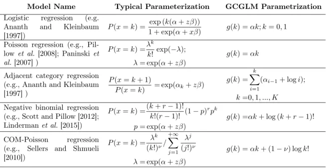
Table 2.1: Special cases of GCGLM. For all models, the GCGLM parametrization for

θ is only associated with the slope θ(x) = βx, and the intercept α is absorbed into the g(·) function. In all cases we have g(k) =−∞ outside the stated support of the distribution. Whenever unspecified, the support of the distribution and the domain of the g(·)function are non-negative integers _N.

Model Name Typical Parameterization GCGLM Parametrization

Logistic regression (e.g.

Ananth and Kleinbaum

[1997])

P(x=k) = exp (k(α+zβ))

1 + exp(α+xβ) g(k) =αk;k= 0,1

Poisson regression (e.g., Pil-low et al. [2008]; Paninski et

al.[2007] ) P(x=k) =λ k k! exp(−λ); λ= exp(α+zβ) g(k) =αk

Adjacent category regression (e.g., Ananth and Kleinbaum [1997] ) P(x=k+ 1) P(x=k) = exp(αk+zβ) g(k) = k X i=1 (αi−1+ logi); k=0,1, ..., K

Negative binomial regression (e.g., Scott and Pillow [2012];

Lindermanet al.[2015]) P(x=k) =(k+r−1)! k!(r−1)! (1−p) r_pk p= exp(α+zβ) g(k) =αk+ log (k+r−1)! COM-Poisson regression

(e.g., Sellers and Shmueli

[2010]) P(x=k) = λ k (k!)ν/ +∞ X j=1 λj (j!)ν λ= exp(α+zβ) g(k) =αk+ (1−ν) logk!

trial r ∈ {1, ..., R}, the PLDS assumes that the spike activity of neurons is a noisy Poisson observation of an underlying low-dimensional latent state zrt ∈ Rp,(where

pN), such that:

xrti|zrt∼Poisson exp

c>_i zrt+di . (2.4) Here C = c1 ... cN >

∈ _RN×p _{is the factor loading matrix mapping the latent}

state zrt to a log rate, with time and trial invariant baseline log rate d ∈RN. Thus

the vector Czrt+d denotes the vector of log rates for trial r and timet. Critically,

the latent state zrt can be interpreted as the underlying signal of interest that acts

Gaussian dynamical system (to capture temporal correlations):

zr1 ∼ N(µ1, Q1)

zr(t+1)|zrt∼ N(Azrt+bt, Q),

(2.5)

where µ1 ∈ Rp and Q1 ∈ Rp×p parameterize the initial state. The transition matrix A ∈ _Rp×p _{and innovations covariance Q ∈}

Rp×p parameterize the dynamical state

update. The optional termbt∈Rp allows the model to capture a time-varying firing

rate that is fixed across experimental trials. The PLDS has been widely used and has been shown to outperform other models in terms of predictive performance, including in particular the simpler Gaussian linear dynamical system [Mackeet al., 2011].

The PLDS model is naturally extended to what we term the generalized count linear dynamical system (GCLDS) by modifying equation (2.4) using a GC likelihood:

xrti|zrt∼ GC c>i zrt, gi(·)

. (2.6)

Where gi(·) is the g(·) function in (2.1) that models the dispersion for neuron i.

Similar to the GLM, for identifiability, the baseline rate parameter d is dropped in (2.6) and we can fix g(0) = 0. As with the GCGLM, one can recover preexisting models, such as an LDS with a Bernoulli observation, as special cases of GCLDS (see Table 2.1).

2.4

Inference and learning in GCLDS

As is common in LDS models, we use expectation-maximization to learn parameters Θ = {A,{bt}t, Q, Q1, µ1,{gi(·)}i, C} . Because the required expectations do not

2010], we required an additional approximation step, which we implemented via a variational lower bound. Below we detailed the VBEM algorithm we use for the model

2.4.1

E-step: variational inference with dual optimization

First, each E-step requires calculating p(zr|xr,Θ) for each trial r ∈ {1, ..., R} (the

conditional distribution of the latent trajectories zr={zrt}1≤t≤T, given observations

xr = {xrti}1≤t≤T,1≤i≤N and parameter Θ). For ease of notation below we drop the

trial index r. These posterior distributions are intractable, and in the usual way we make a normal approximation p(z|x,Θ)≈q(z) = N(m, V).

One simple way to achieve this is by Laplace approximation, i.e. we approximate posterior mean by the mode of the joint distribution m = arg maxzp(z|x,Θ) and

approximate posterior variance by the negative inverse Hessian of the log-likelihood evaluated at the mode V = −(∇2_{logp(z|x,Θ))}−1_|

z=m. Laplace approximation is

simple and fast, but does not have a theoretical guarantee and can be inaccurate. Here we identify the optimal (m, V) by maximizing a variational Bayesian lower bound (the so-called evidence lower bound or “ELBO”) over the variational parameters m, V as: L(m, V) = Eq(z) log p(z|Θ) q(z) +Eq(z)[logp(x|z,Θ)] (2.7) = 1 2 log|V| −tr[Σ −1_{V]−(m−µ)}T_Σ−1_(m−µ) +X t,i Eq(zt)[logp(xti|zt)] +const,

which is the usual form to be maximized in a variational Bayesian EM (VBEM) algorithm [Buesing et al., 2014]. Here µ∈ _RpT _{and Σ∈}

RpT×pT are the expectation

negative Kullback-Leibler divergence between the variational distribution and prior distribution, encouraging the variational distribution to be close to the prior. The second term involving the GC likelihood encourages the variational distribution to explain the observations well. The integrations in the second term are intractable (this is in contrast to the PLDS case, where all integrals can be calculated analytically [Buesinget al., 2014]). Below we use the ideas of Emtiyaz Khanet al.[2013] to derive a tractable, further lower bound. Here the term Eq(zt)[logp(xti|zt)] can be reduced

to: Eq(zt)[logp(xti|zt)] = Eq(ηti)[logpGC(x|ηti, gi(·))] =Eq(ηti) " xtiηti+gi(xti)−logxti!−log K X k=0 1 k!exp(kηti+gi(k)) # , (2.8)

where ηti = cTi zt. Denoting νtik =kηti+gi(k)−log(k!) = kcTi zt+gi(k)−logk!,

(2.8) is reduced to Eq(ν)[νtixti −log(

P

0≤k≤Kexp(νtik))]. Since νtik is a linear

trans-formation of zt, under the variational distribution νtik is also normally distributed

νtik ∼ N(htik, ρtik). We have htik = kcTi mt +gi(k)−logk!, ρtik = k2cTi Vtci, where

(mt, Vt) are the expectation and covariance matrix of zt under variational

distribu-tion. Now we can derive a lower bound for the expectation by Jensen’s inequality:

Eq(νti) " νtixti −log X k exp(νtik) # ≥htixti−log K X k=1

exp(htik+ρtik/2) =:fti(hti, ρti).

(2.9) Combining (2.7) and (2.9), we get a tractable variational lower bound:

L(m, V)≥ L∗(m, V) =Eq(z) log p(z|Θ) q(z) +X t,i fti(hti, ρti). (2.10)

For computational efficiency, we complete the E-step by maximizing the new evi-dence lower boundL∗ _{via its dual [Emtiyaz Khanet al., 2013]. Full details are derived}

in section 2.4.4.

2.4.2

M-step: analytical form

The M-step then requires maximization ofL∗ _{overΘ. We have two sets of parameters}

to optimize in the M-step. One set is for the dynamical system(A,{bt}Tt=1, Q, Q1, µ1),

the other is for the observation (C,{gi(·)}i). Similar to the PLDS case, the set

of parameters involving the latent Gaussian dynamics (A,{bt}Tt=1, Q, Q1, µ1) can be

optimized analytically [Macke et al., 2011]. Then, the parameters involving the GC likelihood (C,{gi}i) can be optimized efficiently via convex optimization techniques

[Boyd and Vandenberghe, 2009].

The part of the likelihood about the dynamical system has the form

L2(A, Q, Q1, µ1) = R X r=1 Eq(zr) " −1 2(zr1−µ1) T_Q−1 1 (zr1−µ1) −1 2 T−1 X t=1 (zr(t+1)−Azrt−bt)TQ−1(zr(t+1)−Azrt−bt) −1 2log|Q1| − T −1 2 log|Q| #

Since everything is quadratic with respect to z, the expectation can be calculated analytically. Moreover, all the parameters can be optimized analytically in close

form. ˆ µt= 1 R R X r=1 E(zr1), t= 1, ..., T ˆ Q0 = 1 R R X r=1 E(zr1) + (E(zr1)−µˆ1)(E(zr1)−µˆ1)T ˆ AT ={ R X r=1 T−1 X t=1 E (zrt−µˆt)(zrt−µˆt)T }−1 R X r=1 T−1 X t=1 E (zr(t+1)−µˆt+1)(zrt−µˆt)T ˆ bt=ˆµt+1−Aˆµˆt, t= 1, ..., T −1 ˆ Q= 1 R(T −1) R X r=1 T−1 X t=1 E[(zr(t+1)−Aˆzrt−bˆt)(zr(t+1)−Aˆzrt−bˆt)T]

The part of the likelihood about the observation can be written as

L1(C, g) = N X i=1 " X t=1,...,T r=1,...,R yrti(cTi mrt) +gi(yrti) −log(1 + K X k=1 1 k!exp(k(c T i mrt) +gi(k) + 1 2k 2 cT_i Vrtci)) #

This part is concave and can be optimized efficiently using convex optimization tech-niques.

2.4.3

Practical concerns

In practice we initialize our VBEM algorithm with a Laplace-EM algorithm, and we initialize each E-step in VBEM with a Laplace approximation, which empirically gives substantial runtime advantages, and always produces a sensible optimum. With the above steps, we have a fully specified learning and inference algorithm, which we now use to analyze real neural data.

2.4.4

Dual optimization for E-step

Below we detail the dual optimization we used in the E-step. This part is rather technical and can be skipped for dis-interested readers.

We first introduce the “vectorized” notation for the GCLDS model. Note that in the E-step the inference is separable across trials, so for ease of notation, we only consider one single trial and drop the trial index r. We assume N neurons observed duringT time bins. Denotezt as thep-dimensional latent variable and and xt as the

N-dimensional observation, respectively.

z:=       z1 .. . zT       ,x:=       x1 .. . xT      

The prior can be summarized as a multi-variate Gaussian distribution:

p(z) =N(µ,Σ) where µ=          µ1 Aµ1+b1 .. . AT−1_µ 1+ PT−1 t=1 AT −1−t_b t          , Σ−1 =       Q−₀1+AT_Q−1_{A A}T_Q−1 Q−1_{A Q}−1 _+AT_Q−1_{A A}T_Q−1 . .. . .. . ..       .

The likelihood has the form p(x|z) =Y t,i p(xti|ηti) p(xti|ηti) =GC(xti|ηti, gi(·)) η:=Wz W =blk-diag(C, ..., C),

where we stack all the ηti in η = (η11, ..., η1N, ...., ηT1, ..., ηT N) ∈ RN T. The log

likelihood reads: logp(z,x)∝ − 1 2(z−µ) T_Σ−1_{(z−µ) +}X t,i [xtiηn+gi(xti)−log( X k 1 k!exp(kηti+gi(k)))] −X t,i log(xti!)− 1 2log|Σ|

In the E-step we make a Gaussian approximation to the posterior:

p(z|x)≈q(z) =N(z|m, V).

The variational lower bound reads: L(m, V) = ˆ q(z) log p(z,x) q(z) dz =1 2(log|V| −tr[Σ −1_{V]−(m−µ)}T_Σ−1_(m−µ)) +X t,i Eq(ηti)[logp(xti|ηti)]− 1 2log|Σ|+ dT 2 .

under the variational distribution

νtik∼ N(htik, ρtik).

Therefore we can re-write the termEq(x)[logp(xti|ηti)] and find a lower bound of the

term by Eq(ηti)[logp(xti|ηti)] =Eq(ηti) " xtiηti+gi(xti)−log(xti!)−log( X k 1 k!exp(kηti+gi(k))) # =Eq(νti) " νtixti −log( K X k=0 exp(νtik)) # ≥htixti −log( K X k=0 Eq(νti)(exp(νtik))) =htixti −log( K X k=0 exp(hnk+ρnk/2))

where νti = (νti1, ..., νtiK). We always have νti0 = ρti0 = 0. For the other variables

define

ν = (ν11, ν12, ..., ν1N, ..., νT1, ..., νT N)T,

and define h and ρ similarly. We then have the constraints h := ˜Wm+ ˜d

where ˜

W =W ⊗(1,2, ..., K)T ˜

d=1T×1 ⊗(g1(1)−log 1!, ..., g1(K)−logK!, ...., gN(1)−log 1!, ..., gN(K)−logK!)T

where ⊗ is the Kronecker product. Applying this lower bound and setting νti0 = ρti0 = 0, we get the evidence lower bound (ELBO)

L∗(m, V,h, ρ) =1 2(log|V| −tr[Σ −1_{V]−(m−µ)}T_Σ−1_(m−µ)) +X t,i " 1{xti>0}htixti −log(1 + K X k=1

exp(htik+ρtik/2))

#

the variational inference can now be cast as the optimization problem:

max m,V,h,ρ L ∗ (m, V,h, ρ) subject to V 0 h= ˜Wm+ ˜d ρ=diag( ˜W VW˜T)

Following Emtiyaz Khan et al.[2013], we can solve the dual problem min

α,λm,V,h,ρmax L(m, V,h, ρ) +α

T_{(h−W˜m−d) +˜} 1

2λ

T_{(ρ−diag( ˜W VW˜}T_)),

whereα, λ∈_RT N K _{are the Lagrange multipliers. The unique maximizer with respect}

to(m, V)is given by

m∗ =µ−Σ ˜WTα

Maximization over(h, ρ)is also available in close form. Collecting the term containing (h, ρ). for f∗ to be finite, we need to enforce the constraint αtik = λtik−1{xti=k}.

Therefore, we can express everything in terms of λ

f_ti∗(λti) =max h,ρ α T tihti+λTtiρti/2 + " 1{xti>0}htixti −log(1 + K X k=1

exp(htik+ρtik/2)

#

=

K

X

k=1

λtiklogλtik+ (1− K X k=1 λtik) log(1− K X k=1 λtik). Denotingy˜ti = (1{xti=1},1{xti=2}, ...,1{xti=K})andy˜= (˜y11, ...,y˜1N, ...,y˜T1, ...,y˜T N),

the dual problem is reduced to min λ D(λ) subject to λtik >0 K X k=1 λtik <1, t = 1, ..., T, n= 1, ..., N, k = 1, ..., K where D(λ) := 1 2(λ−y˜) T_{W˜Σ ˜W}T_{(λ−y˜)−( ˜W µ+ ˜d)}T_{(λ−y˜)−} 1 2log|Bλ|+ X t,i f_ti∗(λti)

and the gradient of the dual reads

D0(λ) = ˜WΣ ˜WT(λ−y˜)−W µ˜ −d˜− 1 2diag(W B −1 λ W T₎₋X n f_ti∗0(λti)

2.5

Model evaluation by leave-one-neuron-out error

To evaluate the goodness-of-fit of the LDS models, we use leave-one-neuron-out pre-dictive error. The idea is to split the data into training trials and testing trials. We

first use training trials to learn the model parameter Θ. Then for test data, each time we drop one neuron, use the other neurons to get the posterior distribution of the latent variables, and then compute the posterior distribution of the left out data. Specifically, denote xi

r = (xr1i, ..., xrT i) as the spike train of neuron i for trial

r, x−_ri = (x1_r, ...,xi_r−1,xi_r+1, ....,xn_r)as the spike train for trial r with neuron i left out. We compute the posterior distribution

p(xrti|x−ri) =

ˆ

p(xrti|zr)p(zr|x−ri)zr (2.11)

wherep(zr|x−ri)is approximated with variational distribution and the integration can

be reduced to a one-dimensional numerical integration since xrti only depend on zr

through cT

i zrt. We compute the mean square error of the predicted firing rate and

the predictive log likelihood of the predicted firing rate.

2.6

Experiments

2.6.1

Simulation examples

To demonstrate the generality of the GCLDS and verify our algorithmic implementa-tion, we first simulated four sets of data with binary, (nearly) Poisson, under-dispersed and over-dispersed observations by generating GCLDS model with4different g func-tions for the GC distribution.

• Binary: g(k) =−1.9k for k=0,1;

• Nearly Poisson: g(k) =−1.9k for k =0,1...,10; • Underdispersed: g(k) = −0.4k2_{+ 1.5k for k =0,...,5;}

• Overdispersed: g(k) = 0.2k2 _{−2.1k for k=0,...,5.}

Here we set g(k) = −∞ when k is out of the scope of the definition, implying zero probability of generating an observation of k. Those g functions are selected to generate a small firing rate, which mimics the real neural data setting.

For each scenario we perform 50 independent experiments, each with 50training trials and 10 testing trials. We randomly generate the model parameters and make sure that the latent signals are strong enough. For all simulations we use 30neurons with3latent dimensions. For each neuron, we perturb its owng function by a random linear function to obtain a variable baseline rate. Here we compare the performance of PLDS and GCLDS, both with 3 latent dimensions. For GCLDS we restrict the

gi(·) functions to be the same across all neurons up to a linear function.

Table 2.2 shows the leave-one-neuron-out performance. We observe that GCLDS and PLDS has comparable MSE although GCLDS outperforms a little, which makes sense since even though PLDS has model specification, it can still capture the mean firing rate well as long as the data can be explained by low-dimensional subspace. In terms of log likelihood, GCLDS significantly outperforms PLDS for all but the nearly Poisson case.

2.6.2

Real data analysis

We analyze recordings of populations of neurons in the primate motor cortex during a reaching experiment (G20040123), details of which have been described previously [Yu et al., 2009; Macke et al., 2011]. In brief, a rhesus macaque monkey executed 56 cued reaches from a central target to 14 peripheral targets. Before the subject was cued to move (the go cue), it was given a preparatory period to plan the upcoming reach. Each trial was thus separated into two temporal epochs, each of which has been

Setting Binary Poisson Underdispersed Overdispersed MSE PLDS 0.124(0.001) 0.199(0.004) 0.156(0.001) 0.259(0.008) GCLDS 0.123(0.001) 0.198(0.004) 0.156(0.001) 0.246(0.004) Improve 0.001(0.000) 0.001(0.001) 0.000(0.000) 0.013(0.007) NLL PLDS 0.434(0.002) 0.481(0.003) 0.453(0.002) 0.517(0.003) GCLDS 0.397(0.002) 0.481(0.003) 0.449(0.002) 0.512(0.003) Improve 0.037(0.002) -0.000(0.000) 0.004(0.000) 0.005(0.000) Table 2.2: Simulation result for PLDS and GCLDS. Showing the leave-one-neuron-out mean square error (MSE) and negative log likelihood (NLL) for PLDS and GCLDS, as well as the improvement of GCLDS over PLDS. Results are averaged across 50 independent repeats with standard error showing in parentheses.

suggested to have their own meaningful dynamical structure [Petreska et al., 2011; Churchland et al., 2012]. We separately analyze these two periods: the preparatory period (1200ms period preceding the go cue), and the reaching period (50ms before to 370ms after the movement onset). We analyzed data across all 14reach targets, and results were highly similar; in the following for simplicity we show results for a single reaching target (one 56 trial dataset). Spike trains were simultaneously recorded from 96 electrodes (using a Blackrock multi-electrode array). We bin neural activity at 20ms. To include only units with robust activity, we remove all units with mean rates less than1spike per second on average, resulting in81units for the preparatory period, and 85 units for the reaching period. As we have already shown in Figure 2.1, the reaching period data are strongly under-dispersed, even absent conditioning on the latent dynamics (implying further under-dispersion in the observation noise). Data during the preparatory period are particularly interesting due to its clear cross-correlation structure.

To fully assess the GCLDS model, we analyze four LDS models –(i) GCLDS-full: a separate function gi(·) is fitted for each neuroni ∈ {1, ..., N}; (ii) GCLDS-simple: