HAL Id: hal-02314418
https://hal.archives-ouvertes.fr/hal-02314418
Submitted on 12 Oct 2019
HAL
is a multi-disciplinary open access
archive for the deposit and dissemination of
sci-entific research documents, whether they are
pub-lished or not. The documents may come from
teaching and research institutions in France or
abroad, or from public or private research centers.
L’archive ouverte pluridisciplinaire
HAL
, est
destinée au dépôt et à la diffusion de documents
scientifiques de niveau recherche, publiés ou non,
émanant des établissements d’enseignement et de
recherche français ou étrangers, des laboratoires
publics ou privés.
A Data Augmentation Approach for Sampling Gaussian
Models in High Dimension
Yosra Marnissi, Dany Abboud, Emilie Chouzenoux, Jean-Christophe Pesquet,
Mohamed El-Badaoui, Amel Benazza-Benyahia
To cite this version:
Yosra Marnissi, Dany Abboud, Emilie Chouzenoux, Jean-Christophe Pesquet, Mohamed El-Badaoui,
et al.. A Data Augmentation Approach for Sampling Gaussian Models in High Dimension. EUSIPCO
2019 - 27th European Signal Processing Conference, Sep 2019, La Corogne, Spain. �hal-02314418�
A Data Augmentation Approach for Sampling
Gaussian Models in High Dimension
Y. Marnissi
(1), D. Abboud
(1), E. Chouzenoux
(2), J-C. Pesquet
(2), M. El-Badaoui
(1,3)and A. Benazza-Benyahia
(4)1
SAFRAN TECH, Groupe Safran, 78772 Magny Les Hameaux Cedex, France.
2
Center for Visual Computing, INRIA, CentraleSupélec, University Paris-Saclay, 91190 Gif sur Yvette, France.
3
University of Lyon, UJM-St-Etienne, LASPI, EA3059, F-42023, Saint-Etienne, France.
4
University of Carthage, SUP’COM, COSIM Lab., 2083 El Ghazala Ariana, Tunisia.
Abstract—Recently, methods based on Data Augmentation (DA) strategies have shown their efficiency for dealing with high-dimensional Gaussian sampling within Gibbs samplers compared to iterative-based sampling (e.g., Perturbation-Optimization). However, they are limited by the feasibility of the direct sampling of the auxiliary variable. This paper reviews DA sampling algorithms for Gaussian sampling and proposes a DA method which is especially useful when direct sampling of the auxiliary variable is not straightforward from a computational viewpoint. Experiments in two vibration analysis applications show the good performance of the proposed algorithm.
Index Terms—Data augmentation, Auxiliary variables, MCMC, Gaussian, Correlation, Bayesian.
I. INTRODUCTION
This paper deals with the problem of sampling from a high
dimensional Gaussian distribution1 with mean m ∈RQ and
precision matrix G=PJ
j=1Gj ∈RQ×Q such that
(∀j ∈ {1, . . . , J}) Gj =H⊤jΛjHj, (1)
where for j ∈ {1, . . . , J}, Λj ∈ RNj×Nj is a positive
semi-definite matrix and Hj ∈ RNj×Q. Very often, we do not
have direct access to the mean m but only to the potential
vector p = Gm. We further assume that the latter reads
p = PJ
j=1Gjmj where for j ∈ {1, . . . , J}, mj ∈ RQ.
Gaussian sampling arises in linear inverse problems involving Gaussian or hierarchical Gaussian models. In such situations, Gaussian simulation is mostly needed as a sampling step at each iteration of a Markov Chain Monte Carlo algorithm e.g., Gibbs samplers. Typical applications are image deconvolution [1], super-resolution [2], inpainting [3], [4], weather forecast-ing [5], etc.
The problem of high dimensional Gaussian sampling has been widely addressed in the literature and several solu-tions have been proposed. Typical approaches for large scale Gaussian simulation are inspired from deterministic iterative optimization techniques. The most known ones are samplers
1Note that the degenerate Gaussian distribution case (i.e., whose covariance
matrix is positive semi-definite but not with full rank) is considered as a proper distribution w.r.t. the restriction of the Lebesgue measure to the image subspace of this covariance matrix. This amounts to replacing inverse with generalized inverse and determinant with pseudo-determinant in the computation of the density function. Throughout this article, for deficient rank positive semi-definite matrices,(···)−1 will denote the generalized inverse.
derived from the Perturbation-Optimization strategy [2], [3], [6] and matrix splitting optimization [4], [7]. These two families of methods are good candidates for efficient Gaussian sampling in large scale problems since they avoid the storage and the factorization of large matrices. However, they both require solving a linear system at each iteration which can be computationally expensive. Thereby, when implemented through a Gibbs sampler, they may turn out to be less efficient;
in particular, when G depends on some target parameters
evolving along the algorithm. Recently, new sampling strate-gies have been proposed as alternatives to optimization based Gaussian sampling [8], [9], [10]. By adding some auxiliary variables, the authors demonstrate, in several inverse problems applications, that sampling becomes much easier in the new augmented space. In the following, we will use the term Data Augmentation (DA) sampling to designate any sampling algorithm that introduces auxiliary variables [11].
In this paper, we are interested in DA strategies for Gaussian sampling in large scale problems. Section II reviews recent DA Gibbs algorithms that allow to separate heterogeneous correla-tions in the covariance matrix. The DA Gibbs sampler, initially introduced in [9], is extended to handle the limitation of state-of-the-art techniques. Section III compares the performance of the different DA samplers in vibration analysis applications. Finally, some conclusions are drawn in Section IV.
II. DATAAUGMENTATION STRATEGY FORGAUSSIAN
SAMPLING
A. Principle
The difficulty of Gaussian sampling arises particularly when
the matrices (Hj,Λj)1≤j≤J cannot be diagonalized in the
same basis. Therefore, it is desirable to separate heterogeneous matrices in order to facilitate sampling. This has been success-fully achieved using DA strategies [8], [9], [10]. Specifically,
auxiliary variables u ∈ RP, are added to the model2 with
a predefined joint distribution with density q(x,u). The key
requirement is that q(x,u) should define a valid probability
density function (i.e. non-negative whose integral with respect
2Initially, the model contains the main variable x ∼ N(m,G−1)and
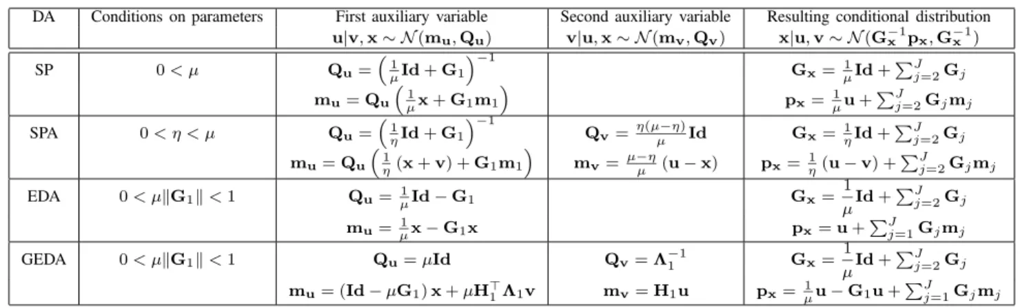
TABLE I: Conditional distributions of xand of the auxiliary variables.
DA Conditions on parameters First auxiliary variable Second auxiliary variable Resulting conditional distribution u|v,x∼ N(mu,Qu) v|u,x∼ N(mv,Qv) x|u,v∼ N(G− 1 x px,G− 1 x ) SP 0< µ Qu= 1 µId+G1 −1 Gx= 1 µId+ PJ j=2Gj mu=Qu 1 µx+G1m1 px= 1 µu+ PJ j=2Gjmj SPA 0< η < µ Qu= 1 ηId+G1 −1 Qv= η(µ−η) µ Id Gx=1 ηId+ PJ j=2Gj mu=Qu 1 η(x+v) +G1m1 mv= µ−η µ (u−x) px= 1 η(u−v) + PJ j=2Gjmj EDA 0< µkG1k<1 Qu=1 µId−G1 Gx= 1 µId+ PJ j=2Gj mu= 1 µx−G1x px=u+ PJ j=1Gjmj GEDA 0< µkG1k<1 Qu=µId Qv=Λ− 1 1 Gx= 1 µId+ PJ j=2Gj mu= (Id−µG1)x+µH1⊤Λ1v mv=H1u px= 1 µu−G1u+ PJ j=1Gjmj
touandxequals1). This is ensured if the marginalization of
q(x,u) with respect to u andx gives rise to valid marginal
probability density functions q(x) = R
RMq(x,u) du and
q(u) = R
RQq(x,u) dx [11]. At each iteration of the new
Gibbs sampler, the Gaussian sampling step is replaced by two sampling steps from the conditional distributions of the two variables and in an arbitrary order. The DA strategy is said to be exact if the introduction of auxiliary variables does not alter the initial model. This is achieved if the marginal
distribution q(x) is equal to the target distribution (being in
our case the Gaussian distribution of meanmand covariance
matrix G−1
). Hereafter, examples of recently proposed DA methods are reviewed. These methods can be categorized into approximate and exact DA samplers.
B. Related works
Without loss of generality, we consider the problem of
eliminating the coupling induced byG1in the precision matrix
(the methods can be easily generalized to other coupling
matrices following the same lines). To this end, q(x,u) is
selected, so as, in the new augmented space, G1 is no more
coupled directly with xbut only intervenes through auxiliary
variables. Table I summarizes the state-of-the-art DA strategies proposed for the aforementioned purpose.
1) Approximate DA: The split (SP) sampler [10], is derived from the deterministic variable splitting optimization strategy. The main idea is to split the initial model into the product of a pair of density functions, for example the likelihood and the prior distribution. Each function is expressed with respect
to one variable namely the main variable x and the splitting
variable u. A quadratic function φ(x,u;µ) = 1
µkx−uk
2
withµ >0, is added to the model to control the discrepancy between the two parameters. This function can be particularly interpreted as the minus-logarithm of their joint distribution.
Consequently, for the purpose of eliminating G1 in the
distribution of x, the resulting conditional distributions are
summarized in Table I. It can be noticed that the additional splitting variables make the different precision matrices appear
in two separate distributionsq(x|u)andq(u|x). However, this
splitting strategy is not exact which means that the resulting
distribution of x is only an approximation of the target one.
The two distributions only coincide in the limiting case when
the varianceµof the Gaussian splitting variable goes to zero.
However, the smaller µ, the higher the correlation between
samples. Such a scenario can jeopardize the mixing properties of the samples. In [10], the authors propose to introduce an
additional auxiliary variable v in the SP Gibbs sampler to
decrease the correlation betweenxandu. This allows the use
of higher values for µ, with the aim to better approach the
exact target distribution. The resulting sampler is known as the Split And Augmented (SPA) sampler. It is worth noting that SPA Gibbs sampler reduces to SP Gibbs sampler by
integrating outv. Further discussions and theoretical results on
approximate DA Bayesian approaches can be found in recent works [12], [13].
2) Exact DA: Exact DA (EDA) strategies have been derived in [8], [9], [14] to cope with both the high dimensionality and the strong correlation existing between the target parameters in high dimensional Gaussian models. These methods are related to half-quadratic optimization approaches proposed in [15], as established in [8]. The resulting hierarchical Gibbs scheme is summarized in the third row of Table I. Note that
only the matrices (Gj)j6=1 are still directly coupled to the
main variable in the new augmented space, similarly to the splitting DA methods. Eventually, the advantage of this DA method compared to SP and SPA, is that the former is exact. Nevertheless, contrary to the EDA sampler, the splitting DA strategies are not restricted to Gaussian models (see [10] for examples).
C. A generalized exact DA strategy for Gaussian models
The main interest of DA strategies is that, in the new augmented space, the sampling task is much easier than direct sampling from the initial model. This can be achieved provided
that the sampling step from q(u|x) does not introduce a
too high computational cost in the algorithm. Ultimately, the reviewed DA methods fail when direct sampling is not feasible. The feasibility depends on the structure of matrix
G1. To alleviate these limitations, we propose a new DA Gibbs
sampler that will be designated as the GEDA algorithm. More
precisely, two auxiliary variables u∈RQ and v ∈RN1 are
• x∼ N m,G−1, • u|x∼ N x,Γ−1, • v|u∼ N H1u,Λ− 1 1 ,
whereGandmtake the form presented in Section I and
Γ= 1
µId−G1, 0< µkG1k<1. (2)
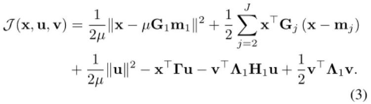
Since v is independent from x conditionally to u, the joint
density distribution of these variables reads q(x,u,v) =
q(v|u)q(u|x)q(x). In particular, its minus logarithm can be
expressed up to an additive constant as follows:
J(x,u,v) = 1 2µkx−µG1m1k 2 +1 2 J X j=2 x⊤Gj(x−mj) + 1 2µkuk 2 −x⊤Γu−v⊤Λ1H1u+ 1 2v ⊤Λ 1v. (3)
The resulting conditional distributions ofx,uandvare given
in Table I. It can be seen that the interest behind introducing
the variableuis to eliminateG1 in the covariance matrix of
x conditionally to uwhile the introduction of the variablev
aims at facilitating the sampling ofuso that this variable can
be drawn directly without requiring intensive computations.
Similarly, the sampling step forvcan be performed efficiently
for a large instance of inverse problems for which Λ1 is
diagonal or has a simple structure.
Table II compares the different DA methods with respect to the feasibility of a direct sampling of the auxiliary variables when Λ1 = αId with α > 0. This may particularly arises
in linear inverse problems with decorrelated Gaussian noise. It can be noted that, in contrast with the approximate DA samplers, EDA sampler makes direct sampling possible when
the matrix H1 is the product of two matrices belonging to
diagonal, tight frame [16] or circulant families [9, Section 3.4]. This may arise for example in image recovery applications
when H1=PMwhereP is a tight frame analysis operator
and M is a convolution matrix with periodic boundary
con-dition. Non-trivial forms of H1 arise in several applications
such as compressive sensing [17], spectroscopy [18], image reconstruction [16], etc. In such situations, only the GEDA algorithm enables efficient sampling of all variables (see Section III-B for an example).
TABLE II: The feasibility of direct sampling ifΛ1
=αId.
H1 SP SPA EDA GEDA
Diagonal X X X X
Tight frame X X X X
Circulant X X X X
Product X X
Non-trivial form X
It is worth noting that, the EDA algorithm can be viewed as a particular instance of the proposed Gibbs algorithm by
marginalizing with respect tov. Thus, one might prefer to use
the EDA sampler rather than the GEDA if direct sampling of the auxiliary variables is tractable. Indeed, it is expected
that this marginalization improves the mixing properties of the samples. The proposed GEDA method can be used as an alternative to the EDA algorithm when direct sampling of the auxiliary variable is not feasible. In Section III, we show that the GEDA sampler still performs well when compared to the reviewed DA strategies even if direct sampling of the auxiliary variable is feasible. Interestingly and following the same lines as for the EDA sampler in [9], the GEDA algorithm can be also easily generalized to cases when the distribution of interest is non-Gaussian but its minus-logarithm density comprises a quadratic function with respect to some variables controlling the mean and/or the variance (e.g., location or scale mixture of Gaussian, Gaussian Markov random fields etc) by including these variables in the Gibbs scheme.
III. APPLICATION TO VIBRATION ANALYSIS
A. Order tracking
In a rotating machine, each mechanical component gener-ates unique vibration patterns as the machine opergener-ates. It is a common practice to monitor these components by analyzing their vibratory level, provided that the system kinematic is known (i.e. the frequencies of the monitored components). This reduces to an amplitude and phase modulations estima-tion problem. Such problem is known in the literature as order tracking [19].
1) Problem formulation: The order tracking problem can be addressed with the following dynamic model [20]:
y(n) =
K
X
k=1
sk(n) +w(n) (4)
where n ∈ {1, . . . , N} denotes time index, k ∈ {1, . . . , K}
labels the sinusoidal components sk. In model (4), y(n) ∈
R2 contains the real and the imaginary part of the
Hilbert transform of the measured vibration data, sk(n) =
Ck(n)xk(n) where Ck(n) ∈ R2×2 is given by Ck(n) =
[Ψ(φk(n)),Ψ(φk(n) + π2)], φk(n) is the instantaneous
phase of the kth component, Ψ(.) = [cos(.),sin(.)]⊤ and
w(n) is assumed to be a zero-mean Gaussian noise with
variance σ2
. Let y = [y(1)⊤, . . . ,y(N)⊤]⊤ and x =
[x⊤
1, . . . ,x⊤K]⊤ where xk = [xk(1)⊤, . . . ,xk(N)⊤]⊤.
Fur-thermore, let ak = [[xk(1)]1, . . . ,[xk(N)]1]⊤ and bk =
[xk(1)]2, . . . ,[xk(N)]2]⊤. Note that ak and bk can be
ex-tracted fromxk using some suitable sparse matrices P1 and
P2 i.e. ak = P1xk and bk = P2xk. To perform the
estimation, it is advantageous to consider the low-frequency or, equivalently, the slow-varying part of the amplitude and phase modulations profiles. This can be practically made by adding the following smoothing prior:
(∀k∈ {1, . . . , K}) g(xk)∝γNk exp −γkx⊤kBxk (5)
whereB=P⊤1L⊤LP1+P2⊤L⊤LP2such thatL=δId+∇,
∇ ∈ RN×N is a circulant matrix associated to a discrete
Laplacian filter, δ > 0 is a small constant that ensures the
positive definiteness of L⊤L, and γ
k >0 is a regularization
distribution for σ2
and Gamma prior distributions for the
regularization parameters i.e., σ2
∼ IG(a, b) and for every
k ∈ {1, . . . , K}, γk ∼ G(ak, bk) where a, b, ak, bk are
positive constants that are set in practice to small values to ensure weakly informative priors. From the observation and
the prior models, the posterior of the target signal xreduces
to a Gaussian one with precision matrix and potential given respectively by G= 1 σ2C ⊤C+M, p= 1 σ2C ⊤y (6)
whereC= [C1, . . . ,CK],Ckis a block matrix formed by the
matricesCk(1). . . ,Ck(N)andMis a block matrix formed
by the matricesγ1B, . . . , γKB. Note that the precision matrix
in (6) reduces to (1) by setting J = 3,H1=C,Λ1=
1
σ2Id,
and, for everyj∈ {2,3},Λjis the diagonal matrix containing
γk andHj is the block matrix formed by K blocks ofLPj.
The posterior distributions of the remaining parameters are given by:
• σ2|x,y∼ IG a+N, b+12kCx−yk2,
• ∀k∈ {1, . . . , K} γk|xk∼ G ak+N, bk+x⊤kBxk
2) Gibbs samplers: SinceMandCcannot be diagonalized in the same basis, direct sampling from the Gaussian distri-bution with parameters (6) is intractable. Thus, we propose to resort to DA strategies. In particular, we aim at eliminating the
coupling induced by C⊤C in the posterior precision matrix
of x. Since CC⊤ = PK
k=1CkC⊤k =K Id, kCC⊤k = K
and direct sampling of the Gaussian auxiliary variables in the EDA Gibbs sampler is straightforward. For the SP and SPA algorithms, an explicit expression of the covariance matrix of
the auxiliary variable ucan be found by using the Woodbury
matrix identity so that, similarly to EDA, direct sampling of the auxiliary variables can be fulfilled easily. Regarding the sampling step of the target signal, it can be noted that for
all the DA strategies, the different components a1, . . . ,aK,
b1, . . . ,bK are uncorrelated given the auxiliary variables and their covariance matrices are circulant so that they can be drawn easily, in an independent manner, in the Fourier domain. As it is complicated to sample from the conditional
distributions of the parameters σ2
, γ1, . . . , γK subject to the
auxiliary variables, we follow [9] i.e., we instead sample from their marginalized distributions by partially collapsing all the auxiliary variables.
3) Performance comparison on synthetic data: We consider
a synthetic signal containing3 components with time-varying
instantaneous amplitudes and frequencies and their 4 first
integer multiple harmonics over a duration of 4 seconds and
at a sampling frequency of 3,000Hz. Thus, K = 15 and
N = 12,000. A Gaussian noise with variance σ2
= 7605 is artificially added to the signal so that the initial
signal-to-noise ratio is equal to 0 dB. The hyperparameters a, b,
ak, bk, k ∈ {1, . . . , K} are set to zero to ensure
non-informative priors. Simulations were performed on an Intel(R) Core(TM) i5-6300U CPU @ 2.40 GHz, using a Matlab 2014 implementation. The spectrogram of the noisy signal and the
estimated one (using the empirical average of 1,000samples
generated by the GEDA algorithm after convergence) are shown in Figure 1. 0.5 1 1.5 2 2.5 3 3.5 Time [s] 0 500 1000 1500 Frequency [Hz] 0.5 1 1.5 2 2.5 3 3.5 Time [s] 0 500 1000 1500 Frequency [Hz] (a) SNR= 0 dB (b) SNR=18.64 dB
Fig. 1: Spectrogram. (a) Noisy signal (b) Estimated signal.
Figure 2 shows the evolution of the parameter σ2
with respect to the computational time for the considered DA
sampling algorithms for different values of µ and η (given
here up to a multiplicative factorσ2
). One can see that the best convergence speed is achieved by the different samplers for
very small value ofµwhile SP appears to converge towards a
wrong distribution for higher values ofµ(i.e.,µ>0.1). These
results are consistent with the findings highlighted in [10]. The remaining samplers share a roughly similar convergence speed.
0 200 400 600 800 1000 1200 Time [s] 0.7 0.8 0.9 1 1.1 1.2 1.3 1.4 2 104 SP ( =10-6) SP ( =0.01) SP ( =0.1) SPA ( =10-6, =10-12) SPA ( =0.01, =10-6) EDA ( =0.01K) EDA ( =0.9K) GEDA ( =0.01K) GEDA ( =0.9K) Fig. 2: Evolution ofσ2
with respect to time.
Table III shows the mixing results for the DA algorithms in terms of time per iteration after the burn-in period, Mean Square Jump (MSJ) in stationarity and MSJ per second. Note
that the MSJ is estimated with an empirical average over1,000
samples after convergence similarly to [9]. It can be noted that all algorithms have the same iteration cost and share good mixing properties except SP and SPA for low values
of µ. Compared to SP, the addition of auxiliary variables in
SPA enhances slightly the mixing but the two algorithms still explore less efficiently the parameter space compared to exact DA samplers. In particular EDA is twice more efficient than SP and SPA. Moreover, it appears that the best mixing properties
for EDA and GEDA are achieved for large values of µ. It is
worth noting that EDA shows mixing properties slightly better than GEDA which is expected since EDA is a marginalized version of GEDA. However, one should recall that GEDA covers a wider scope of Gaussian sampling problems than EDA. It follows that GEDA seems to be a good candidate to replace EDA in Gaussian sampling when the covariance matrix does not satisfy the requirements in [9].
TABLE III:Mixing results of DA samplers. T[s] MSJ MSJ/T SP (µ= 10−6) 0.14 12.86 86.39 SP (µ= 10−2) 0.14 415.48 2836.19 SPA (µ= 10−6,η= 10−12) 0.15 12.93 80.63 SPA (µ= 10−2,η= 10−6) 0.15 433.64 2776.62 EDA (µ= 0.01K) 0.12 153.02 1275.16 EDA (µ= 0.9K) 0.12 817.32 6438.12 GEDA (µ= 0.01K) 0.14 149.48 1067.71 GEDA (µ= 0.9K) 0.13 598.01 4326.98
B. A more complex illustrative scenario
For illustrative purpose, we consider the compressive sens-ing model in Section 4.2 of [17] to reconstruct a vibration
signal of length Q = 30,000 acquired in a spur Gearbox
from a low number of measurementsN = 5,000. The
recon-struction requires to specify a sparse representation operator for the vibration signal which is here achieved by the Fast Fourier transform. Following [17], to promote compressible solutions, the Fourier coefficients of the signal are assumed to be i.i.d according to a zero mean scale mixture of Gaus-sian distributions with a Gamma mixing density, which is equivalent to the Student’t distribution. Thus, the problem amounts to a Gaussian sampling problem where the precision
matrix is of the form (1) with J = 2, H1 = SΨ where
Ψ is the inverse Fast Fourier transform operator and S is a
random Gaussian projection matrix with a reduced dimension
N = 5,000, and Λ1 andG2 are diagonals. It is clear that as
H1 has a non-trivial form, in particular because Sis neither
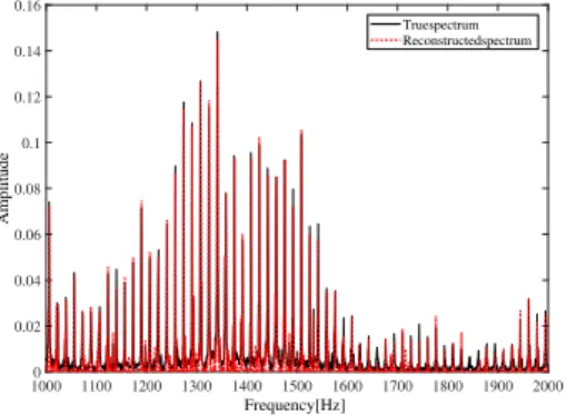
diagonal, nor circulant nor a tight frame, the state-of-the-art DA techniques fail to sample directly the target variables, while the proposed GEDA method can still be applied. Figure 3 shows the initial and the reconstructed spectra with the
GEDA sampler (µ = 0.9kG1k−
2
) in the frequency band
(1,000,4,000)Hz. The algorithm needs about1,000iterations
to converge which is equivalent approximately to500seconds.
1000 1100 1200 1300 1400 1500 1600 1700 1800 1900 2000 Frequency [Hz] 0 0.02 0.04 0.06 0.08 0.1 0.12 0.14 0.16 Amplitude True spectrum Reconstructed spectrum
Fig. 3: Target and reconstructed spectra.
IV. CONCLUSION
This paper has reviewed recent DA strategies for Gaussian sampling and proposed a new one that can be used as an alter-native to the method introduced in [9] when direct sampling of
the auxiliary variable is not feasible. It relies on adding two auxiliary variables: while the first auxiliary variable aims at facilitating the sampling of the target signal, the second one enables direct sampling of the first auxiliary variable. Simula-tion results in two vibraSimula-tion analysis applicaSimula-tions indicate the good performance of the considered DA Gibbs samplers.
REFERENCES
[1] C. Fox and R. A. Norton, “Fast sampling in a linear-Gaussian inverse problem,”SIAM-ASA J. Uncertain., vol. 4, no. 1, pp. 1191–1218, 2016. [2] C. Gilavert, S. Moussaoui, and J. Idier, “Efficient Gaussian sampling for solving large-scale inverse problems using MCMC,”IEEE Trans. Signal Process., vol. 63, no. 1, pp. 70–80, 2015.
[3] G. Papandreou and A. L. Yuille, “Gaussian sampling by local perturba-tions,” inProc. Adv. Neural Inf. Process. Syst. (NIPS 2010), (Vancouver, Canada), pp. 1858–1866, 6-11 Dec 2010.
[4] A.-C. Barbos, F. Caron, J.-F. Giovannelli, and A. Doucet, “Clone MCMC: Parallel High-Dimensional Gaussian Gibbs Sampling,” inProc. Adv. Neural Inf. Process. Syst. (NIPS 2017), (Long Beach, CA), pp. 5020–5028, 4-9 Dec 2017.
[5] Y. Gel, A. E. Raftery, and T. Gneiting, “Calibrated probabilistic mesoscale weather field forecasting: The geostatistical output pertur-bation method,”J. A. Stat. Assoc., vol. 99, no. 467, pp. 575–583, 2004. [6] O. Féron, F. Orieux, and J.-F. Giovannelli, “Gradient Scan Gibbs Sam-pler: an efficient algorithm for high-dimensional Gaussian distributions,” IEEE Journal of Selected Topics in Signal Process., vol. 10, no. 2, pp. 343–352, 2016.
[7] M. Johnson, J. Saunderson, and A. Willsky, “Analyzing Hogwild Parallel Gaussian Gibbs sampling,” inProc. Adv. Neural Inf. Process. Syst. (NIPS 2013), (Harrahs and Harveys, Lake Tahoe), pp. 2715–2723, 5-10 Dec 2013.
[8] Y. Marnissi, E. Chouzenoux, J.-C. Pesquet, and A. Benazza-Benyahia, “An auxiliary variable method for langevin based MCMC algorithms,” in Proc. IEEE Stat. Signal Process. Workshop (SSP 2016), (Palma de Mallorca, Spain), pp. 297–301, 26-29 Jun. 2016.
[9] Y. Marnissi, E. Chouzenoux, A. Benazza-Benyahia, and J.-C. Pesquet, “An Auxiliary Variable Method for Markov Chain Monte Carlo Algo-rithms in High Dimension,”Entropy, vol. 20, no. 2, 2018.
[10] M. Vono, N. Dobigeon, and P. Chainais, “Split-and-augmented Gibbs sampler-Application to large-scale inference problems,” arXiv preprint arXiv:1804.05809, 2018.
[11] D. A. Van Dyk and X.-L. Meng, “The art of data augmentation,” J. Comput. Graph. Stat., vol. 10, no. 1, pp. 1–50, 2001.
[12] M. Vono, N. Dobigeon, and P. Chainais, “Asymptotically exact data augmentation: models, properties and algorithms,”arXiv preprint arXiv:1902.05754, 2019.
[13] S. Sisson, Y. Fan, and M. Beaumont, “Overview of approximate Bayesian computation,”arXiv preprint arXiv:1802.09720, 2018. [14] R. Cavicchioli, C. Chaux, L. Blanc-Féraud, and L. Zanni, “ML
estima-tion of wavelet regularizaestima-tion hyperparameters in inverse problems,” in Proc. IEEE Int. Conf. Acoust., Speech Signal Process. (ICASSP 2013), (Vancouver, Canada), pp. 1553–1557, 26-31 May 2013.
[15] J. Bect, L. Blanc-Féraud, G. Aubert, and A. Chambolle, “A l1-unified variational framework for image restoration,” in Proc. European Con-ference on Computer Vision (ECCV 2004), (Prague, Czech Republic), pp. 1–13, 11-14 May 2004.
[16] N. Pustelnik, A. Benazza-Benhayia, Y. Zheng, and J.-C. Pesquet, “Wavelet-based image deconvolution and reconstruction,” Wiley Ency-clopedia of Electrical and Electronics Engineering, 2016.
[17] R. Fuentes, C. Mineo, S. G. Pierce, K. Worden, and E. J. Cross, “A probabilistic compressive sensing framework with applications to ultrasound signal processing,” Mech. Syst. Signal Process., vol. 117, pp. 383–402, 2019.
[18] P. J. Brown, T. Fearn, and M. Vannucci, “Bayesian wavelet regression on curves with application to a spectroscopic calibration problem,”J. A. Stat. Assoc., vol. 96, no. 454, pp. 398–408, 2001.
[19] H. Vold, H. Herlufsen, M. Mains, and D. Corwin-Renner, “Multi axle order tracking with the Vold-Kalman tracking filter,”Sound Vib., vol. 31, no. 5, pp. 30–35, 1997.
[20] R. Turner and M. Sahani, “Probabilistic amplitude and frequency demodulation,” in Proc. Adv. Neural Inf. Process. Syst. (NIPS 2011), (Granada Spain), pp. 981–989, 12-17 Dec 2011.