econ
stor
www.econstor.eu
Der Open-Access-Publikationsserver der ZBW – Leibniz-Informationszentrum Wirtschaft
The Open Access Publication Server of the ZBW – Leibniz Information Centre for Economics
Nutzungsbedingungen:
Die ZBW räumt Ihnen als Nutzerin/Nutzer das unentgeltliche, räumlich unbeschränkte und zeitlich auf die Dauer des Schutzrechts beschränkte einfache Recht ein, das ausgewählte Werk im Rahmen der unter
→ http://www.econstor.eu/dspace/Nutzungsbedingungen nachzulesenden vollständigen Nutzungsbedingungen zu vervielfältigen, mit denen die Nutzerin/der Nutzer sich durch die erste Nutzung einverstanden erklärt.
Terms of use:
The ZBW grants you, the user, the non-exclusive right to use the selected work free of charge, territorially unrestricted and within the time limit of the term of the property rights according to the terms specified at
→ http://www.econstor.eu/dspace/Nutzungsbedingungen By the first use of the selected work the user agrees and declares to comply with these terms of use.
zbw
Leibniz-Informationszentrum WirtschaftLiesenfeld, Roman; Richard, Jean-François
Working Paper
Improving MCMC Using Efficient
Importance Sampling
Economics working paper / Christian-Albrechts-Universität Kiel, Department of Economics, No. 2006,05
Provided in cooperation with:
Christian-Albrechts-Universität Kiel (CAU)
Suggested citation: Liesenfeld, Roman; Richard, Jean-François (2006) : Improving MCMC Using Efficient Importance Sampling, Economics working paper / Christian-Albrechts-Universität Kiel, Department of Economics, No. 2006,05, http://hdl.handle.net/10419/22010
Improving MCMC Using Efficient Importance
Sampling
by
Roman Liesenfeld, Jean-François RichardEconomics Working Paper
No 2006-05
Improving MCMC Using Ecient Importance Sampling
Roman Liesenfeld∗
Department of Economics, Christian-Albrecht-Universität, Ohlshausenstr. 40-60, 24118 Kiel, Germany
Jean-François Richard
Department of Economics, University of Pittsburgh, 4S01 Wesley W. Posvar Hall, Pittsburgh, PA 15260, USA
May 15, 2006
Abstract
This paper develops a systematic Markov Chain Monte Carlo (MCMC) framework based upon Ecient Importance Sampling (EIS) which can be used for the analysis of a wide range of econometric models involving integrals without an analytical solution. EIS is a simple, generic and yet accurate Monte-Carlo integration procedure based on sampling densities which are chosen to be global approximations to the integrand. By embedding EIS within MCMC procedures based on Metropolis-Hastings (MH) one can signicantly improve their numerical properties, essentially by providing a fully automated selection of critical MCMC components such as auxiliary sampling densities, normalizing constants and starting values. The potential of this integrated MCMC-EIS approach is illustrated with simple univariate integration problems and with the Bayesian posterior analysis of stochastic volatility models and stationary autoregressive processes.
Keywords: Autoregressive models, Bayesian posterior analysis, Dynamic latent variables; Gibbs sam-pling, Metropolis Hastings; Stochastic volatility
∗Corresponding author. Tel.: +49-431-8803810; fax: +49-431-8807605. E-mail address:
1 Introduction
Monte Carlo (MC) simulation methods are widely used to analyze a broad range of econometric models involving integrals for which no analytical solution exist. Excellent surveys on MC based econometric methods are available (see, e.g., Geweke, 1999, Gilks et al., 1996, Gourieroux and Mon-fort, 1996 and Stern, 1997). Two methods dominate the eld. Importance Sampling (IS) was introduced in econometrics by Kloek and van Dijk (1978) and widely used in the eighties. It became progressively supplanted by Markov Chain Monte Carlo (MCMC) in the nineties. Seminal papers are that of Gelfand and Smith (1990), proposing MCMC techniques for Bayesian computations, and that of Tanner and Wong (1987) who introduced data augmentation for the treatment of latent variables. The main argument against the use of IS is the potential non-existence of the MC sampling variance which could lead to disastrous properties of IS estimates (see, e.g., Geweke 1989, 1999 and more re-cently Koopman and Shephard, 2004). In the present paper we will argue that the IS and MCMC are more closely related than generally recognized and, in particular, that the argument of non-existing variance which contributed to the relative demise of IS also apply to Metropolis-Hastings (MH) pro-cedures which represent, together with the Gibbs-sampling techniques, the most widely used MCMC algorithms.
The fundamental insight which motivates the present paper lies in the observation that the sam-pling properties of both IS and MCMC critically depend upon the adequacy of an auxiliary sampler
m, meant to approximate (up to a proportionality constantc) a density kernel ϕwhich needs to be
numerically integrated (by itself and/or to compute expectations of functions of interest). Ecient Importance Sampling (EIS), as proposed by Richard and Zhang (2006), provides a generic and es-sentially automated Least Squares (LS) procedure to construct such (near) optimal approximations within a preassigned parametric class M of auxiliary samplers. Whence we should be able to
fa-cilitate the design as well as improve the sampling properties of MCMC by relying upon auxiliary EIS regressions to constructm. Most importantly, once it is recognized how closely related EIS and
MCMC are, the key issue of deciding which approach to use for a particular application becomes one of objective comparison, of respective ease of implementation and statistical adequacy within the context of that application, not of subjective preference for one method or the other.
Typically, EIS can be expected to have comparative advantages at integrating out high-dimensional dynamic latent variables. The eciency of EIS in such situations is illustrated by its application for the computation of the likelihood of various dynamic latent variable models (see, e.g., in Bauwens and Hautsch, 2003, Bauwens and Galli, 2005, Jung and Liesenfeld, 2001, and Liesenfeld and Richard
2003a, 2003b, 2005a). In particular, in the context of highly correlated latent variables, EIS can usefully be interpreted as a single block MCMC step, providing an ecient solution to the slow convergence of MCMC in such context. On the other hand, intricate Bayesian posterior densities are generally more amenable to MCMC integration. This is illustrated by the estimation of stochastic volatility (SV) models where MCMC and EIS are combined together along this lines (subsection 6.1). Moreover, even in applications where MCMC is unequivocally to be preferred, we will illustrate ways of embedding EIS auxiliary steps within the MCMC algorithm in order to facilitate the con-struction of the MCMC sampler and, in the process, to improve its convergence properties. This will be illustrated in the context of the MCMC analysis of the roots of stationary AR models (subsection 6.2).
The rest of the paper is organized as follows. In section 2, we review the principles of the MC integration procedures under consideration. Section 3 and 4 contain a brief description of the EIS technique and MCMC approaches, respectively. In particular we, discuss how EIS can usefully be combined with MCMC. This is illustrated in section 5 and 6 with numerical examples. In particular, we discuss two simple univariate integration problems (subsections 5.1 and 5.2), a Bayesian analysis of a SV model (subsection 6.1), and a MCMC analysis of the roots of AR models (subsection 6.2). Section 7 concludes.
2 MC Integration
Consider a continuous random variableXwith support∆⊂RT. We assume that its density function
f(x) is characterized by a density kernelϕ(x)whose integrating constant on∆is unknown. That is
to say
f(x) =c−1·ϕ(x), with c=
Z
∆
ϕ(x)dx. (1)
Letg(x) denote aϕintegrable function. Its expectation on f is given by Ig =Ef[g(X)] = R ∆g(x)ϕ(x)dx R ∆ϕ(x)dx . (2)
IS and MCMC (MH) are commonly used to evaluate such (ratios of) integrals. In order to motivate our paper, we rst present both methods in a particular way which serves highlighting their intrinsically close relationship. Technical assumptions validating these methods are extensively discussed in the literature see, e.g., Geweke (1989) and Robert and Casella (1999) and are omitted here.
All MC integration techniques discussed in the present paper share the characteristic that they rely upon a sequence of `primary' draws {x˜i; i: 1→S}. While IS uses these draws as such, MH
requires additional auxiliary steps based upon uniform draws in order to determine which of the primary draws are to be deleted, retained and/or repeated. For the purpose of the present discussion it proves convenient to reinterpret both IS and MCMC estimates of Ig as (randomized) weighted
sums of functions of the primary draws, say
¯ Ig = PS i=1g(˜xi)·α x˜(i),˜vi PS i=1α x˜(i),v˜i , (3)
wherex˜(i) = (˜xj; j: 1→i)andv˜i denote additional auxiliary uniform draws as required for MCMC.
Implicitly assuming convergence, let m(xi) denote the stationary margin of x˜i. IS relies upon i.i.d.
draws with weights
α x(i), vi ≡ω(xi) = ϕ(xi) m(xi) . (4)
There exists a wide variety of MH techniques, some of which are described below, which generally result in assigning integer values to the αs, which then represent the number of times a primary
draw appears in the average. Letµ denote the (stationary) joint distribution of the auxiliary draws (˜x(i),˜vi). Additional notations are:
¯ ω = Em[ω(˜xi)] =c (5) a(xi) = Eµ α(˜x(i),v˜i)|x˜i =xi (6) ¯ a = Em[a(˜xi)]. (7)
Next, we reinterpret I¯g as an MC-estimator of Ig, i.e. a decision rule which maps a ϕ-integrable
function g into a point estimate of its expectation on the density f. Under standard technical
conditions consistency ofI¯g obtains under the following condition
Em g(˜xi)· a(˜xi) ¯ a =Em g(˜xi)· ω(˜xi) ¯ ω =Ig (8)
for allϕ-integrable g. This implies that there exists a constantb >0 such that
a(xi) =b·ω(xi), m−a.s. , (9)
where b accounts for dierent implicit normalization rules associated with the weights. It follows
that Varµ α x˜(i),v˜i = Em Var α x˜(i),v˜i |x˜i +b2Varm[ω(˜xi)] (10) ≥ b2Varm[ω(˜xi)].
Due to the complex correlation structure of the α weights under MH schemes, the inequality
(10) does not necessarily imply that IS is more ecient than MH. However, it has two fundamental implications which motivate the present paper: (i) The criticism commonly raised against IS that Var[ω(X)] might not exist also applies to MH, a fact which is often ignored in the literature on
MCMC and cannot by itself justify the demise of IS procedures. (ii) More constructively, as we shall discuss further below, the MH α weights are produced by accept-reject steps based upon ratios of
the formω(x)/c, wherecis a calibration constant. Ecient MH algorithms are those for which the
distribution of these ratios is tightly concentrated around one. Since, as discussed further below, EIS is designed with that objective, we should be able to facilitate the construction of MH algorithms and improve their eciency by relying upon EIS auxiliary steps to construct the MH samplers. This is the objective of the present paper.
3 Ecient Importance Sampling (EIS)
The EIS procedure proposed by Richard and Zhang (2006) hereafter RZ provides a generic aux-iliary LS algorithm to select an ecient sampler within a preassigned class M. For low-dimensional
problems it approximates the integrandϕ(x) itself a density kernel by a kernelk(x, a) fora∈A.
The correspondence between kand mis given by m(x;a) = k(x, a)
χ(a) , with χ(a) =
Z
X
k(x, a)dx. (11)
A (near) optimal value of a obtains by solving the following auxiliary generalized LS (GLS)
problem ˆ a= arg min a∈A q(a), q(a) = Z X d2(x, a)·ω(x, a)·m(x;a)dx, (12) with d(x, a) = lnϕ(x)−γ−lnk(x, a), (13) ω(x, a) = ϕ(x) m(x;a), (14)
and γ = lnc is an intercept (calibrating constant), which is included in a for the ease of notation.
For a tentative valueˆaj ∈A, an MC estimate of q(a) is given by
¯ qS(a|ˆaj) = 1 S S X i=1 h lnϕ ˜ xji −γ−lnk ˜ xji, a i2 ·ω ˜ xji,ˆaj , (15)
where{x˜ji; i: 1→S}are i.i.d. draws fromm(x; ˆaj).
Letˆaj+1 denote the value ofawhich minimizes q¯S(a|ˆaj). EIS consists of recursively solving the
GLS problem associated with Equation (15) until a xed point solution obtains whereby ˆaj+1 'ˆaj.
In earlier iterations where the variance ofωcan be large, it is recommended to set theωs in Equation
(15) equal to one in order to avoid imbalances due to large weights. Note that if k belongs to the
exponential family of distribution, then it can be parameterized in such a way that lnk is linear in aand the search for ˆais reduced to a sequence of linear LS problems.
High-dimensional EIS requires that ϕ(x) be partitioned into low-dimensional components in
ac-cordance with a natural (model based) sampling preordering (allowing for parallel sequences under appropriate conditional independence assumptions as for panels). Letx be partitioned conformably
with such a preordering into x = (x1, . . . , xL), under the convention that x` is to be drawn
condi-tionally on x(`−1) = (x1, . . . , x`−1). Bothϕand m are factorized accordingly into
ϕ(x) = L Y `=1 ϕ` x(`) (16) m(x;a) = L Y `=1 m` x` |x(`−1), a` . (17)
Note thatϕ`(x(`)), which is given by the model specication, is typically not a kernel for the
condi-tional densityf`(x`|x(`−1)). Kernels forf` obtain from the backward recursion
ϕ∗` x(`) =ϕ` x(`) · Z ϕ∗`+1(x(`+1))·dx`+1, (18)
together withϕ∗L=ϕL. Such integrals are generally intractable which is precisely why MC is used.
However, a similar recursive procedure can be applied to a sequence of (operational) IS approximating kernelsk`(x(`), a`). Specically, the ratio ϕ/m can be rearranged as
ϕ(x) m(x;a) =χ1(a1)· L Y `=1 ϕ `(x(`))·χ`+1(x(`), a`+1) k`(x(`), a`) , (19) together with χ`+1 x(`), a`+1 = Z k`+1(x(`+1), a`+1)dx`+1 (20)
and χL+1(·) ≡ 1. Step j of the EIS xed point search for ˆa = (ˆa`; ` : 1→ L) consists of drawing
full trajectories {x˜ji`; ` : 1 → L; i : 1 → S} from the previous step sampler m(x; ˆaj) and solving
a backward sequence of auxiliary GLS problems of the form given by Equation (15) whereby
High-dimensional EIS implicitly assumes thatϕ`·χ`+1 and, therefore,k` only depend on a
su-ciently low-dimensional subvector of x(`) in accordance with conditional independence assumptions
built into the model under consideration (see RZ, 2006 for full notation and implementation details). It is important to emphasize that in order to secure smooth convergence towards a xed point solution ˆa, all EIS iterations are to be run under Common Random Numbers (CRNs), in the sense
that all auxiliary draws{x˜ji; i: 1→n}are constructed as transformation of a single set of canonical
draws{u˜i; i: 1→n}, i.e. draws whose densities do not depend ona(for example, uniforms on(0,1)
from which thexs obtain by inversion of the cdf). As discussed in RZ (2006), the use of CRNs also
robusties EIS against outlier draws in the sense that outliers fromm(x; ˆaj)will be highly inuential
in the auxiliary (G)LS problem, as given by Equation (15) and will generate an immediate adjustment inˆaj+1. While the use of CRNs thereby critically contributes reducing the estimated variance ofI¯g,
it obviously does not eliminate the possibility that this variance might actually not exist (whether under EIS or MCMC) as would be the case if the tails ofkare thinner than those ofϕ(examples are
provided below). RZ (2006) propose a simple and highly sensitive test to detect such imbalances. It consists of computing the ratio between two alternative MC estimates of the MC sampling variance of I¯g, one based upon draws from the EIS sampler m(x; ˆa) itself and the other from an alternative
samplerm(x;a0)with articially inated variance (by a factor of 3 to 5). This ratio is given by
Γ2S(ˆa, a0) = ˆ σS2(ˆa, a0) ˆ σ2S(ˆa,ˆa), (21) where ˆ σS2(ˆa, a) = 1 S S X i=1 hd2(˜xai,aˆ)· ϕ(˜x a i) m(˜xai;a), (22) h(c) =e √ c+e−√c−2, (23) and {x˜a
i; i: 1→S} denotes (CRN) draws from m(x;a). (The MC sampling variance of I¯g under a
samplerm(x;a) is given by{R
h[d2(x, a)]ϕ(x)dx}/S, see RZ, 2006.) One might consider calibrating
such a ratio by means of auxiliary MC simulations. Experience suggests that such calibration is hardly necessary as Γ2S rapidly explodes in the presence of even mild imbalances between the tails
of m and those of ϕ. Note that by inating the variance of the sampler m(x;a) used to compute ˆ
σS2(ˆa, a), one increases the probability of drawing points in the potentially critical regions. Hence, in
the presence of a thin-tail problem one would expectσˆ2S(ˆa, a) to increase rapidly with the variance
ofm(x;a). Illustrations are provided in section 5 below.
In conclusion of this brief description of EIS, we ought to mention that, relative to MH, EIS oers an additional degree of exibility which can produce additional and occasionally important eciency
gains in the computation of ratios of integrals such as Ig in Equation (2). Consider rst the case
where g(x) > 0 on X. It is then trivial to compute separate EIS samplers for the numerator and
denominator ofIg (under a single set of CRNs). Specically, letm(x; ˆaN)denote an EIS sampler for
the product g·ϕ and m(x; ˆaD) one for ϕ alone. Let (˜xN i;i : 1 → S) and (˜xDi;i : 1 → S) denote
corresponding sets of draws obtained by transformation of a single set of CRNs. An EIS-2 samplers estimate ofIg is then given by
¯ Ig2 = PS i=1ωN(˜xN i) PS i=1ωD(˜xDi) , (24)
where ωN = ϕ·g/m(·; ˆaN) and ωD = ϕ/m(·; ˆaD). Illustrations of the signicant eciency gains
produced by EIS-2 samplers forg(x) =x withx >0and g(x) =x2 are provided in section 5 below.
A similar idea applies to situations wheng(x) though not strictly positive onX can be decomposed
into the product of a positive function and a remainder. Note that there is no MH counterpart to EIS-2 samplers since MH aims at producing draws from ϕ itself, from which expectations are
evaluated as simple arithmetic means.
4 Markov Chain Monte Carlo (MCMC)
The object of MCMC is to construct an auxiliary Markov Chain whose stationary distribution is the one associated with the density kernelϕ. Such chains include acceptance steps. Whence, in line
with our discussion in section 2, we introduce an explicit distinction between `primary' draws (˜xi)
and `accepted' draws(˜yi). As for EIS, we rst discuss low-dimensional integration problems.
A baseline MH Markov Chain consists of two components: (i) A transition probability density m(x|y);
(ii) An acceptance probabilityρ(x|y) dened as: ρ(x|y) = min ϕ(x) m(x|y) · m(y|x) ϕ(y) ,1 . (25)
Assuming convergence after an initialization run, the MH algorithm proceeds as follows: Condition-ally on the latest accepted draw y˜i, draw x˜i+1 from m(x|y˜i) and accept x˜i+1, i.e. set y˜i+1 = ˜xi+1,
with probabilityρ(˜xi+1 |y˜i). Otherwise, set y˜i+1 = ˜yi. The corresponding MH estimate of Ig is a
simple arithmetic mean over accepted draws
¯ Ig= 1 S S X i=1 g(˜yi). (26)
It trivially corresponds to formula (3) when reformulated in terms of the x˜is with α(˜x(i), vi)
repre-senting the number of time a primary draw was counted in the sum. Note, in particular that a y˜i
which obtains as the outcome ofssuccessive rejections equalsx˜i−s, and that a rejected primary draw
˜
xi receives an α weight of zero. The MH algorithm as dened above is quite general in the sense
that I¯g converges almost surely toward Ig as long as the chain {y˜i} is ergodic (see, e.g. Chib and
Greenberg, 1995 or Robert and Casella 1999).
A special version of MH is the independent MH (see Tierney, 1994), which is widely used in econometrics as a key component of MCMC algorithms. This method, which is most closely related to IS, relies upon auxiliary sampling densities which are independent from previous draws, in which casem(x|y) =m(x). The corresponding acceptance probabilityρ is then given by
ρ(x|y) = min ω(x) ω(y),1 , (27)
with ω(x) = ϕ(x)/m(x). A necessary and sucient condition for ergodicity of a chain from an
independent MH (and hence for convergence) is thatm is almost everywhere positive on the support ∆ofϕ, which is not particularly restrictive per se (see Robert and Casella, 1999, Chapter 6.2). This
being said, the rate of convergence and the eciency of MH critically depends upon how well m
approximatesϕ up to a multiplicative constant cwhich actually cancels out in Equations (25) and
(27). Note, in particular, that the better the approximation ofϕbym, the lower the variation in the
ratio (min{ω(˜x)/ω(˜y),1}), and hence, the higher the average acceptance rate. Furthermore, only for
densitiesm, satisfying
ω(x)<∞ ∀x∈∆,
a fast exploration of the support∆implied by uniform ergodicity of the resulting chain{y˜i}can be
guaranteed (see Robert and Casella, 1999, Chap. 6.3). Without such a strong ergodicity property, which is rarely met in practical applications, the convergence can be very slow. In particular observe, that when m is lighter-tailed than ϕ, the algorithm can get stuck at points in the tails with very
low acceptance rates for new candidate draws, leading to potentially very largeα weights for such
points. Finally, notice the close accordance between the condition for uniform ergodicity and the requirement for a nite MC variance of IS procedures.
It follows that in order to construct (independent) MH algorithms with fast convergence and high eciency, one should select a density m which closely approximates ϕand, in particular, such
that the ratio ϕ/m is bounded. Therefore, subject to the usual thin-tail caveat, an EIS density m which, as discussed in section 2, provides a global LS approximation to ϕ should also result in
dierence between the intrinsic objectives of optimizing an IS procedure and improving the rate of convergence of MH (through faster exploration of∆). Nevertheless, as illustrated below, ecient IS
samplers can signicantly accelerate the convergence of MH.
MH is often used in combination with other (MC)MC techniques. In particular, the combination of independent MH with Accept-Reject (AR) sampling leads to the AR-MH algorithm proposed by Tierney (1994). In the initial AR step of AR-MH, candidates drawn from m are accepted with
probability p(x) = min 1 cω(x),1 , (28)
where c > 0 represents a calibration (tuning) parameter. MH is then applied to the accepted
(primary) drawsx˜i from this initial step, with a probabilityρ modied as follows:
ρ(x|y) = min ϕ(x)·min [ϕ(y), c·m(y)] ϕ(y)·min [ϕ(x), c·m(x)],1 . (29)
The AR-MH algorithm is particularly useful in situations when the precondition for pure AR sampling i.e. the existence of a constantcsuch thatϕ(x)≤c·m(x),∀x∈∆ either is hard to verify or leads
to unacceptably high numbers of rejections. On the other hand, it is obvious that the convergence of an AR-MH algorithm also critically depends upon the constantc. In the absence of operational
optimality criterion for the selection of c, rules of thumb are widely used in applications (see, e.g.,
Jacquier et al., 1994 or Chib and Greenberg, 1995). In contrast, the use of EIS to construct an AR-MH auxiliary samplermoers the additional benet that the tuning parametercis a fully automated
by-product obtained from the estimation of the interceptγ in the EIS regression (15). In particular,
the estimate γˆ captures the average dierence between lnϕ and the EIS approximation lnk(x,aˆ).
Hence, by settingc=χ(ˆa)·eˆγ, one can expect a balanced trade-o between too frequent rejection in
the initial AR-step from high c values and too frequent repetitions in the subsequent MH-step due
to lowc values. Accordingly, automated selection ofc should be an important contribution of EIS
within the AR-MH algorithm which, as illustrated below, can considerably accelerate convergence. In higher dimensional problems, Gibbs sampling (itself an MCMC algorithm) is often used in combination with MH. Gibbs relies upon a partitioning ofxinto low-dimensional components, sayx= (x1, . . . , xL)such that the conditional densitiesf(x` |x\`), wherex\`= (xi;i6=`), are MC tractable,
in the sense that they are either amenable to direct simulation, or can be sampled through MC approximations. Gibbs then repeatedly cycles across the complete set of such conditional densities until convergence obtains. While Gibbs oers the advantage that its low-dimensional components can be easy to draw from, it suers from the fact that high correlations amongxscan dramatically slow
or Shephard and Pitt, 1997). Important examples of such problems are high-dimensional dynamic latent variable models such as SV models, an example of which is discussed below. Bayesian analysis of such models require integrating out a high-dimensional vector λof latent variables in addition to
a vector θ of unknown parameters, in which case x = (θ, λ). Partitioning λinto blocks instead of
individual variables alleviates the high-correlation problem but also complicates approximating the corresponding (block) conditional densities. On the other hand, EIS has proved to be very ecient for (single block) high-dimensional integration of λ | θ (see, e.g., Liesenfeld and Richard, 2003b).
We shall present below a highly ecient Gibbs-EIS-MH combination for the Bayesian analysis of SV models, whereby EIS is used to draw complete (single block) trajectories forλ|θ, and conventional
MH-Gibbs is used to drawθ|λ.
5 Two Univariate Examples
In this section we discuss two simple univariate examples, illustrating how EIS can be used to automate the selection of an MH sampler (within a preassigned class). We show that the performance of such an EIS-MH combination is very close to that of EIS itself. The auxiliary statisticΓS dened
in Equation (21) is used under both EIS-MH and EIS to detect thin-tail problems. We also illustrate the fact that neither EIS nor EIS-MH can match EIS-2 samplers for the estimation of (positive) moments.
5.1 Inverse Gaussian Density
Consider the computation of the mean Ef(x), whenxfollows an inverse Gaussian distributionf with
a density kernel
ϕ(x, θ) =x−3/2e−θ1x−θ2/x, x >0, θ
1 >0, θ2 >0, (30)
where θ = (θ1, θ2)0. The analytical form of the mean is Ef(x) = p
θ2/θ1. Following Robert and
Casella (1999, Chap. 6.4.1) hereafter RC letk be the following gamma kernel
k(x, a) =xκ−1e−x/δ, x >0, κ >0, δ >0. (31)
For MC estimation of Ef(x) based upon independent MH, RC (1999) propose to select a value of
a = (κ, δ)0 which (approximately) maximizes the MH acceptance rate subject to the simplifying
assumption that the mean of the auxiliary samplerm(x;a) coincides with that of f. This requires
that the ratio
ω(x, a) = f(x) m(x;a) ∝x
−κ−1/2e(1/δ−θ1)x−θ2/x (32)
be bounded. The latter requires that1/θ1 < δ and ensures uniform ergodicity. Since the expected
acceptance rate is impossible to compute it has to be approximated by simulation. Forθ1= 1.5 and
θ2 = 2, the optimal value forδ subject to the constraint 1/1.5< δ, as obtained by RC (1999), lies at
the boundaryδ∗ = 1/1.5. The corresponding value for ais given bya∗= (pθ2/θ1/δ∗, δ∗)0.
Note that the procedure described above is not easy to generalize to a wider range of applications. Optimization based upon estimated acceptance rates is a non-trivial and time consuming operation (with a discontinuous objective function). Nor would Ef be generally available in which case the RC
approach would require iterations based upon intermediate estimates of Ef.
In contrast (unconstrained) EIS relies upon trivial bivariate linear auxiliary regression associated with the following expression ford(x, a) as dened in Equation (13):
d(x, a) = −3 2lnx−θ1x− θ2 x −γ−[α1lnx+α2x], (33)
whereα1 =κ−1,α2 =−1/δ, and γ denotes the regression intercept. It should be noted that the
variance ofω(x, a)remains nite even when1/θ1 > δ, in which caseω(x, a)is unbounded. Actually,
the MC variance ofω(x, a)can be expressed in terms of Bessel functions of imaginary argument (see
Gradshteyn and Ryzhik, 1979, 3.471.9). Whence we do not impose the uniform ergodicity condition and, unsurprisingly in view of the RC results, nd that the EIS solutionˆaviolates that condition.
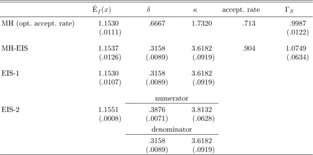
Results are reported in Table 1 for the RC approach based on the optimized acceptance rate and for the corresponding MH-EIS (using 20 EIS iterations to obtain the nal EIS valueˆa). The results which
are reported are sample means and standard deviations based upon 100 independent replications of the complete algorithms, providing a reliable measure of numerical accuracy. Individual runs are based upon S = 5,000 draws. The results of the experiment indicate that the optimized MH
algorithm based on m(x;a∗) and the MH-EIS procedure using m(x; ˆa) perform very similarly with
respect to numerical eciency: while the former has a MC standard deviation of 0.011, the latter has one of 0.013. The acceptance rates for the MH-EIS procedure (90%) is signicantly larger than that for the optimized MH (71%). This indicates that the EIS kernel k(x,ˆa) based on an unconstraint
GLS optimization associated with Equation (33) provides a signicantly better global approximation to ϕ(x, θ) than the kernel k(x, a∗), which is selected subject to the constrained that the ratio (32)
remains bounded. For comparison, we considered the direct EIS estimate of Ef(x) using the same
EIS-sampler as for MH-EIS. The MC standard deviation of this estimate (EIS-1) provided in the third row of Table 1 indicates a numerical eciency which is close to that of the MH procedures.
In order to make sure that the unboundedness ofω(x,aˆ)does not adversely impact the estimation
of Ef(x) we computed the ΓS statistic, as dened in Equation (21), under variance ratios varying
from 5 to 30 (replacing(ˆκ,δˆ) by(ˆκ/q, qδˆ) amounts to multiplying the variance ofm(x; ˆa) byq). We
nd thatΓSremains tightly distributed around one in all cases (only the results forq= 5are reported
in Table 1), indicating the complete absence of adverse thin-tail eects. Clearly, MH-EIS provides a fully operational (and generic) alternative to the RC procedure as well as one which enables us to verify that we can safely relax the boundary condition in this application.
Last but not least, in order to illustrate the exibility and full potential of EIS in the present case, we also computed an EIS-2 samplers estimate of Ef(x) whereby, as described in section 2, separate
EIS samplers (under CRNs) are used to approximatex·ϕandϕ, respectively. The EIS forx·ϕonly
requires adding lnx to d(x, a) in Equation (33) (which represents the EIS for ϕ). The results for
this EIS-2 are reported in the last row of Table 1. Note the large eciency gain with MC-variance reduction by a factor of 150.
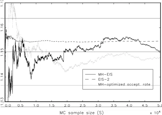
The results discussed above are also conrmed by Figure 1, where we reproduce plots of MC estimates of Ef(x)under increasing sizeS for MH based on optimized acceptance rate, MH-EIS, and
EIS-2. Note that both MH procedures have similar convergence patterns with MH-EIS performing somewhat better. Clearly none of the MH approaches can remotely match the performance of EIS-2.
5.2 Student-t Density
In our second example, we consider the classical pathological problem of approximating a Student-tby
a Normal density. In particular, we focus on the MC estimation of Ef(x2) wheref is a standardized
tdensity with a kernel
ϕ(x, ν) = 1 + x 2 ν−2 −(ν+1)/2 , (34)
such that Ef(x) = 0, and Ef(x2) = 1 for all degrees of freedomν >2. The normal sampling density
kernel under consideration is parameterized as
k(x, a) =e−ax2/2, a >0, (35)
such that Em(x) = 0 and Em(x2) =a−1. Notice thatlimν→∞f(x;ν) =m(x; 1). The EIS univariate
linear regression forϕcorresponds to the following expression ford(x, a) d(x, a) = −1 2(ν+ 1)·ln 1 + x 2 ν−2 −γ−αx2, (36)
Table 2 and Figure 2 summarize the result for EIS and (independent) MH-EIS estimation of Ef(x2). Since draws for MH-EIS need to be from f itself, we use rst an EIS for ϕ as dened by
Equation (36). The maximum number of EIS iterations is conservatively set equal to 100, as low degrees of freedom require more iterations. As in the example of subsection 5.1, we computed also direct EIS-1 estimates of Ef(x2) using the same EIS sampler as for the MH-EIS as well as EIS-2
estimates using dierent EIS samplers for the numerator and denominator of Ef(x2) though based
upon a single set of CRNs (see, fth and sixth row of Table 2). The EIS for the denominator only requires adding lnx2 to d(x, a) in Equation (36). The results in Table 2 are means and standard
deviations from 100 replications of the full estimation procedure, each based upon a sample size
S = 1,000. The ΓS statistic as dened in Equation (21), is computed using the EIS sampler and
another sampler with variance equal to ve times that of the EIS sampler (obtained by setting
a0 = 5/ˆa).
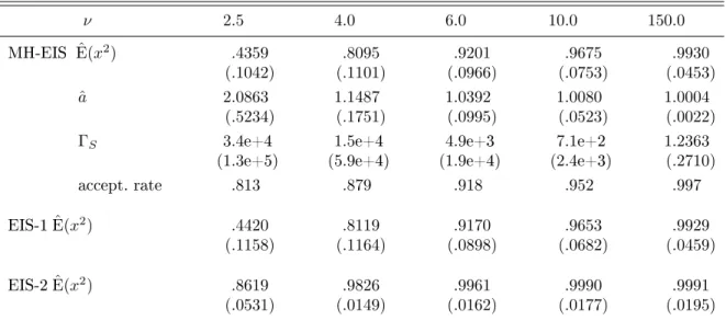
In order to interpret the results for MH-EIS and EIS-1 one needs to account for the fact that low degrees of freedom studenttdensities are signicantly tighter around their mode than a N(0,1)
-density in order to compensate for fatter tails. Therefore, an EIS sampler approximating ϕ will
have smaller variance (ˆa > 1) which will result in greater downward bias when used to evaluate
R
x2ϕ(x, ν)dxin the numerator. Accordingly, decreasing the degrees of freedom ν (fatting the tails)
increases rapidly the downward bias of MH-EIS and EIS-1 estimates of Ef(x2). Under EIS-2 a
dierent sampler is used for that numerator which explains the signicantly lower biases in row 6 of Table 2 (see also the top line in Figure 2).
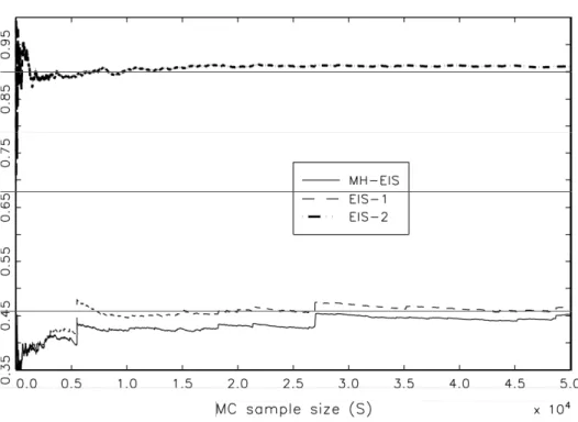
Note that, in sharp contrast with the previous example, the thin-tail issue matters greatly here as indicated by rapidly exploding values ofΓS for low degrees of freedom. Figure 2 conrms our ndings
and indicates that the bias in Ef(x2) estimates under EIS-MH and EIS-1 does not decrease much
for ν= 2.5 as sample sizeS increases up to 50,000. The occasional signicant jumps are the results
of CRN outlier draws aecting the integral of x2ϕ. In contrast, the EIS estimate of the integral
of ϕ remains extremely robust against outliers due to the use of CRNs, as explained in section 3.
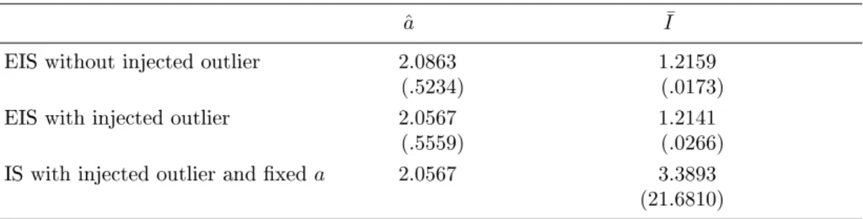
This is illustrated by the results for EIS estimation of I = R ϕ(x, ν)dx reported in Table 3, where
we articially insert a single very large outlier (x = 6 corresponding to a p-value of 9.8e10) in the
rst set of 1,000 N(0,1)draws. The exact value ofI equals 1.2360. Note the minimal impact of that
outlier, except for an increase from 0.017 to 0.027 in the MC standard deviation ofI¯. This is due to
the fact that EIS adjusts eachˆa to the particular set of CRNs being used. The third row of Table
3 indicates that if we prevent such adjustments by keeping ˆaxed, then I¯exhibits the traditional
These two (classical) univariate examples have highlighted several key ndings: (i) MH is subject to the same caveat as (E)IS relative to the thin-tail problem; (ii) Maximally ecient EIS estimation of positive moments obtains when numerator and denominator are treated separately (under a common set of CRNs) note that EIS estimation of the integrals of ϕ and g·ϕ (for g > 0) only require
minimal program changes; (iii) The reliance upon a single set of CRNs from the xed point search for aˆ to the nal estimation of Ig is a critical component of EIS robustness against outliers and
(iv) theΓS statistic dened in Equation (21) eectively discriminates between situations where the
unboundedness ofω(x)is inconsequential (example 5.1) from those where it is critical (example 5.2).
6 Two Higher-dimensional Examples
We now consider two higher-dimensional full-edged applications illustrating how EIS and MH can be combined together for greater numerical eciency.
6.1 Bayesian Analysis of a Stochastic Volatility Model
SV models have received considerable attention in nancial econometrics as specications accounting for the dynamic behavior of the volatility of nancial returns (see Ghysels et al., 1996 or Shephard, 2004). The standard univariate SV model has the form
yt=βeλt/2ut, λt=δλt−1+νvt, t: 1→T, (37)
where yt is the asset return observed in period t, λt is the unobservable log volatility of yt, and
(ut, vt) are i.i.d.N(0,1) variables which are mutually independent. The parameters to be estimated
areθ= (β, δ, ν)0 with the usual stationarity condition that|δ|<1.
Classical and Bayesian inference of the SV model are hindered by the fact that it has no closed-form likelihood. Various (E)IS procedures have been used to perform ML estimation of the SV model (37) and of numerous univariate and multivariate extensions (see, e.g., Sandmann and Koopman, 1998 and Liesenfeld and Richard, 2003b). Alternatively, MCMC algorithms have been proposed for a Bayesian analysis, which avoids the need to compute the likelihood (see, e.g, Jacquier et al., 1994 and Chib et al., 2002). Such an MCMC analysis is typically based on simulation of θ and of the
vector of volatilitiesλfrom their joint conditional distributionf(θ, λ|y)using the Gibbs factorization f(θ|λ, y) and f(λ|θ, y). The simulation of f(λ|θ, y) is most challenging. Most approaches are based
on a `single-move' Gibbs sampling scheme, whereby each element of λ is simulated individually
procedure to simulate λt|λ\t, θ, y element by element. For this purpose, they apply a second-order
(Taylor) expansion around the mean ofλt|λ\t, θ to approximate the log kernel of the target density
lnϕt(λt|λ\t, θ, y) = −[(λt−µt)2/σt2+λt+yt2exp(−λt)/β2]/2, where µt = δ(λt+1+λt−1)/(1 +δ2)
and σt2 =ν2/(1 +δ2). This yields for each period an auxiliary Gaussian sampler mt which can be
used to produce candidate draws for the AR-MH procedure. The mean and variance ofmt are
µ∗t =σt∗2 µt σ2 t +1 2 yt2 β2e −λt(1 +µ t)−1 , σt∗2 = 1 σ2 t + y 2 t 2β2e −λt −1 .
However, the typically high persistence in the λt-process creates a problem for the convergence of
such single-move Gibbs sampling MCMC schemes. To improve the speed of convergence, Shephard and Pitt (1997) suggest a block-sampling technique, that is, a joint simulation of a smaller number of blocks of consecutiveλts.
In view of the numerical eciency of EIS and of the fact that the EIS sampler can be generically be interpreted as a single blocksampler for λ, Liesenfeld and Richard (2005b) propose an
MCMC-EIS Bayesian algorithm combining Gibbs for the parameters given the volatilities and MCMC-EIS for the volatilities given the parameters. In particular, the EIS sampler is used as a proposal density for the AR-MH algorithm to simulate λas a single block fromf(λ|θ, y). The latter is proportional to
ϕ(λ;θ, y) = T Y t=1 exp −1 2 λt+ yt2 β2e −λt +(λt−δλt−1)2 ν2 . (38)
For any givenθ, one can use EIS to construct the following sequential Gaussian sampler
approxima-tion toϕ(λ;θ, y): ϕ(λ;θ, y)'ˆc·m(λ|y, θ,ˆa(θ)) = ˆc· T Y t=1 mt(λt|λt−1, θ,ˆat(θ)), (39)
where ˆat(θ) = ( ˆα1t,αˆ2t) denotes the GLS coecients of λt and λ2t in the sequential EIS auxiliary
regressions. Furthermore,ln ˆc=PT
t=1ˆγt, where theγˆts are the intercepts of the EIS regressions, and
mt is a univariate normal density with kernel
kt(λt;θ,aˆt(θ)) = exp −1 2 (λt−δλt−1)2 ν2 −2 ˆα1tλt+ ˆα2tλ 2 t , (40)
and with varianceσˆ2t =ν2/(1 +ν2αˆ2t) and meanµˆt= ˆσ2t(δλt−1/ν2+ ˆα1t). Whilem would be used
as such for an EIS likelihood evaluation (see Liesenfeld and Richard 2003b), for a Bayesian MCMC analysis one need exact draws fromf(λ|θ, y)for which one can use an AR-MH algorithm based upon
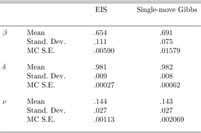
Table 4 and Figure 3 summarizes results of a Bayesian MCMC analysis of the SV model (37) using this single-block EIS sampling procedure for λ, and for comparison, those obtained using the
Shephard and Pitt's (1997) single-move Gibbs sampler described above. The model is applied to the daily exchange rate of the British Pound against the US Dollar from October 1, 1981 to June 28, 1985 (T = 945). (The data set and the prior specication are the same as in Shephard and
Pitt, 1997.) Forlnβ, we use a at prior leading to an inverted chi-squared conditional posterior for β2. An inverted chi-squared prior with a mean of 0.013 and a variance of 0.007 is used for ν2. The
resulting conditional posterior for ν2 is also an inverted chi-squared distribution. Finally, a Beta
prior is assumed for (δ+ 1)/2 with a prior mean for δ of 0.86 and a prior variance of 0.012. The
resulting conditional posterior is non-conjugate and is sampled by an independent MH procedure based on a Gaussian proposal distribution.
Posterior moments are presented in Table 4 together with numerical MC standard errors which are computed with the Parzen based spectral estimator used by Shephard and Pitt (1997). For M
draws of a parameter{θ˜i;i: 1→M} the MC standard error is the square root of
1 M h Γ0+ 2LM LM −1 LM X `=1 K ` LM Γ` i , where Γ`= 1 M M X i=`+1 (˜θi−θ¯)(˜θi−`−θ¯),
withK(·)the Parzen kernel andLMthe bandwidth. The results for both MCMC algorithms are based
on 52,000 Gibbs draws of the parameters, where the rst 2,000 are discarded. The EIS approximation to f(λ|θ, y) is obtained using for the EIS auxiliary regressions a MC sample size of S = 50 and 3
EIS iterations with an initial sampler for theλts given by the sequence of N(δλt−1, ν2) densities (at
the corresponding Gibbs draws of the parameters). The starting values of the parameters used for both MCMC algorithms areβ = 1,δ = 0.9,ν = 0.2. The single-move Gibbs sampler is initialized by
setting allλts to zero and then iterating for the starting values of the parameters on theλs for 1000
iterations. For the MCMC-EIS procedure the rstλ-draw is simulated from the EIS sampler at the
starting values of the parameters.
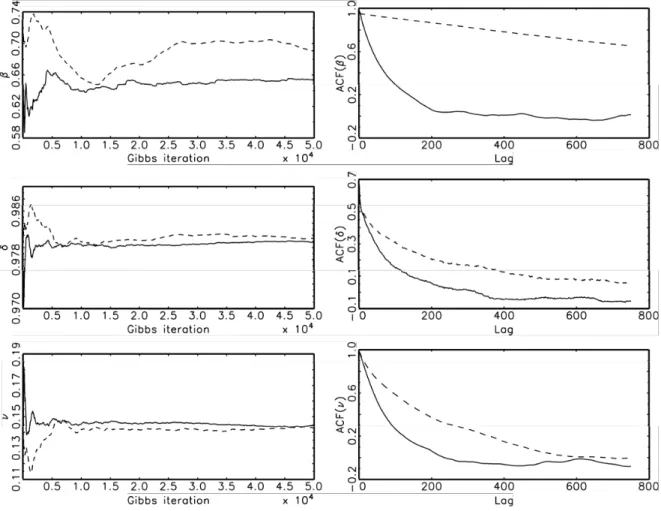
The results in Table 4 show that the the single block MCMC-EIS algorithm performs notably better than the single-move MCMC procedure. In particular, the MC standard errors of the MCMC-EIS estimators are signicantly lower than those of the single-move estimators. This improvement obtained by the single-block EIS sampler is not surprising since the posterior moments for the per-sistence parameter δ (with a mean close to unity) indicate a slowly mixing volatility process. Using
a single-move sampler for the volatilities, this leads typically to a slowly mixing of the MCMC chains on the volatility parameters. This interpretation is conrmed by the autocorrelation function of the
Gibbs draws of parameters and the convergence diagrams, where the MCMC posterior means for the parameters are plotted against the Gibbs iteration (see Figure 3). Notice in particular the se-vere convergence problems of the MCMC posterior mean forβ obtained from the single-move Gibbs
sampler. It appears that it has not converged even after 50,000 iterations, while the MCMC-EIS posterior mean do not need more than 10,000 iterations to reach its convergence level. Finally we notice, that the acceptance rates of the AR-MH EIS algorithm for the simulation ofλ|θ, yturn out to
be 81% (initial AR step) and 80% (subsequent MH step). This reects the close EIS approximation of the kernel of the target densityϕbyˆc·mand indicates thatˆcensures a balanced trade-o between
too frequent rejection in the initial AR-step from highc values and too frequent repetitions in the
subsequent MH-step due to lowc values.
6.2 Bayesian Analysis of a Stationary AR Model
The following last example illustrates the implementation of a fully automated MCMC-EIS algo-rithm in a situation where EIS alone is not operational for a nonlinear parametrization of interest. It consists of the Bayesian posterior analysis of a stationary AR process. Bayesian MCMC analysis of stationary AR processes are found e.g. in Chib and Greenberg (1994,1995). Our analysis diers from theirs in several critical ways. Firstly, it relies on a dierent (nonlinear) parametrization asso-ciated with the roots of the AR process, which are typically the key quantities of interest for such an analysis. Secondly, it makes use of an operational analytical expression for the inverse of the stationary covariance matrix and, relatedly, all draws belong by construction to the stationary region of the parameter space (while in Chib and Greenberg, 1995, primary draws are unconstrained and then accepted or rejected depending upon whether they satisfy or not the stationarity condition). Thirdly, it relies upon an initial EIS approximation to the likelihood function to construct a fully automated and numericlly ecient MCMC posterior analysis.
The model under consideration is
φ(L)yt=yt+φ1yt−1+· · ·+φpyt−p=t, t∼i.i.d.N(0, σ2), t: 1→T, (41)
whereφ(L)is a polynomial in the backshift operatorL. For ease of presentation and without loss of
generality we set σ2 = 1. It is assumed that φ= (φ1, ..., φp)0 lies in the stationary region Bφ, that
is characterized by roots ofφ(L), which lie all outside the unit circle. Following Richard (1977), the
joint stationary density of the initial variablesy[p]= (y1, ..., yp)0 can be written as
where Sp is a lower triangular band matrix with elements sij = φi−j, (j ≤ i) and Rp an upper
triangular band matrix with elementsrij =φp+i−j,(j≥i). The likelihood function is given by
`(φ;y)∝ |Hp|1/2exp n −1 2y 0 [p]Hpy[p] o · " exp n −1 2 T X t=p+1 (yt+φ1yt−1+· · ·+φpyt−p)2 o # . (43)
Assuming a at prior for φ ∈ Bφ, the posterior of the parameters f(φ|y) has a kernel of the form
ϕ(φ;y) =`(φ;y)IBφ, whereIBφis an indicator function of the setBφ. In order to perform a Bayesian
analysis, Chib and Greenberg (1995) simulate from such a posterior using the MH algorithm with an auxiliary samplerm, associated with the Gaussian density kernel for the observationsyt+p, ..., yT
(the term in brackets of Equation, 43).
However, note that theφ coecients are hard to interpret and one would typically have greater
interest in the roots of the process. In order for the transformation from φ into the roots to be
one-to-one, the latter need to be ordered in some appropriate way. An operational solution to this problem consists of factorizing the polynomialφ(L)into ordered binomials. Focusing for the moment
on the case where the orderp is even, sayp= 2r, let φ(L) = r Y j=1 ψj(L) = r Y j=1 (1 +βjL+δjL2), (44)
where the βjs are ordered according to −2 < β1 < · · · < βr < 2. The corresponding stationarity
conditions for ψ= (β1, δ1, ..., βr, δr)0 are given by βj+δj >−1, βj−δj <1, and δj <1. It follows,
that simulated draws of the ψ coecients will automatically satisfy the stationarity restrictions if
they are constrained in the following sequential way: - For βj given all other coecients
max{βj−1,−(1 +δj)}< βj <min{βj+1,(1 +δj)}, with β0 =−2, βr+1= 2; (45)
- For δj given all other coecients
|βj| −1< δj <1. (46)
Obviously, forr >1, theφcoecients are a nonlinear but trivial transformation of theψcoecients,
e.g., forr= 2 we have
φ1 =β1+β2, φ2 =δ1+β1β2+δ2, φ2 =δ1β2+δ2β1, φ4=δ1δ2.
Furthermore, if we partitionψintoψ0 = (ψτ, ψ\0τ), where ψτ is a single parameter, we note thatφis
(45) and (46), provide the key to the proposed MCMC-EIS algorithm for a Bayesian analysis of the
pairs (βj, δj). It also allows for a trivial numerical evaluation of the Jacobian ∂φ/∂ψ0, whose τ-th
column is obtained by increasingψτ by 1 keepingψ\τ xed and computing the resulting dierence
inφ. Accordingly, the proposed MCMC-EIS can be implemented for priors on φas well as priors on ψ.
Based on these preliminaries, the MCMC-EIS algorithm consists of the following key steps: (i) In the rst step, a Gaussian EIS approximation m(φ|y, a)to the posterior associated with the
likelihood (43) is constructed. This requires an auxiliary GLS regression associated with the following expression ford(φ, a) as dened in Equation (13)
d(φ, a) = ln`(φ;y)−γ−α0φ−φ0Σφ, (47)
whereαis ap-dimensional vector andΣa symmetricp×pmatrix. In the application below with p= 6, this regression includes 21 regressors plus one intercept. (For signicantly higherps, one
could embed univariate EIS regressions within the MCMC algorithm instead of computing a single global initial EIS.) In our application we use the prior ofφas initial sampler. Beyond the
sampler itself, this initial EIS step produces two other results which are useful for an ecient MCMC implementation. First, its mode can be used as initial value for the subsequent AR-MH steps, and second, the intercept of the EIS regression can be transformed into an ecient calibration constantcfor the corresponding AR-MH ratios ϕ/[c·m].
(ii) In the next step, the AR-MH algorithm is used to sample individuallyψτ|ψ\τ, y based on the
Gibbs factorization of ψ. Specically, under a uniform prior on ψ the posterior density of a
single ψτ is given by f(ψτ|ψ\τ, y) ∝ ϕ(φ(ψ);y). The AR-MH sampling density for ψτ|ψ\τ, y
is given by the Gaussian conditional density m(ψτ|ψ\τ, y) associated with the EIS sampler
m(φ|y, a). Note that since φ is a linear function of ψτ given ψ\τ, one only needs to evaluate
m(φ|y, a) for three dierent values ofψτ (keepingψ\τ xed) to retrieve the mean and variance
of m(ψτ|ψ\τ, y). The ψτ draws are truncated conformably with the stationarity and ordering
conditions given by Equations (45) and (46). In order to accelerate draws of the truncated
normals one can usefully rely upon interpolation tables for the c.d.f. and inverse c.d.f of the standardized normal.
In order to illustrate the performance of the proposed MCMC-EIS algorithm, we rst reran the application of Chib and Greenberg (1995) for an AR(2) model based on simulated observations. In
particular, we simulated T = 100 observations from an AR(2) with φ1 = −1 and φ2 = 0.5. Since
p= 2, theφ andψ parameters are equivalent and we can benchmark a MCMC-EIS against an EIS
posterior analysis. As in Chib and Greenberg, we use 5,500 MCMC draws of which the rst 500 are discarded. Correspondingly, we use 5,000 draws for EIS. Posterior means and standard deviations are provided in Table 5, together with MC (numerical) standard errors for all relevant estimates. The latter are based upon 100 i.i.d. replications of the complete algorithm. We also provide the MC means and standard errors of the ratiosϕ/[c·m]for MCMC-EIS. The results show that the EIS-step has
eciently normalized these ratios. Furthermore, the EIS as well as the MCMC-EIS algorithm lead to posterior distributions which are centered around the true values of the data generating process. Since Chib and Greenberg (1995) implicitly use an EIS-type algorithm based upon the quadratic part of `(φ;y), their numerical accuracy is similar to the ones obtained here for the MCMC-EIS
algorithm, while the computing time for the latter is absolutely competitive. The CPU times for the entire sampling process using the EIS and MCMC-EIS scheme on a 750 MHz UNIX server are 0.08 and 0.16 seconds, respectively, while Chib and Greenberg report CPU times of 8 minutes for a pure Accept-Reject algorithm and 2 minutes for the MH on a 50MHz PC. Moreover, preliminary investigations suggest that the EIS step has signicantly improved the convergence properties of the MCMC algorithm. For example, we reduced the number of MCMC draws by a factor ten (only 550 draws of which the rst 50 were dicarded) and produced virtually identical estimation results (not presented here) up to 2 or 3 decimals except for the obvious fact that numerical standard errors increased approximately by the factor √10.
Next, for a more stringent test, we repeated the numerical experiment for an AR(p) model with p = 6, using a pair of complex conjugate roots close to the unit circle (±i√0.95), a pair of real
roots (-0.9,0.2) and a double real root (-0.7). The corresponding ordered(βj, δj)-pairs inψare given
by (0, 0.95), (0.7,-0.18) and (1.4,0.49). For p > 1, we can no longer oer an EIS benchmark on
theψ coecients for comparison. The posterior means and standard deviations of ψ together with
MC numerical standard errors and posterior probabilities for complex roots are provided in Table 6. The results are based on 5,500 MCMC draws, where the rst 500 are discarded. CPU time for the entire sampling process is 0.7 seconds. The results indicate that the MCMC-EIS algorithm has accurately produced posterior distributions for theψparameters which are centered around the true
parameter values of the data generating process. (Posterior moments ofφare immediate by-products
of the MCMC-EIS analysis ofψ but are not reported here. When compared with the EIS posterior
moments of φ, they were found to be near identical but numerically less ecient by factor ranging
therefore highly ecient.) Furthermore, a ve fold reduction in the number of MCMC draws leads to virtually identical results (not presented here) except for the corresponding √5-fold increase in
numerical standard errors. Hence, the results suggest that the convergence of MCMC-EIS is very fast and requires fewer draws than typically used in the literature. Again it appears that implementation of an EIS step improved the numerical properties of MCMC, essentially providing (near optimal) fully automated selection of critical MCMC components (starting values, normalizing constant, ecient univariate conditional samplers).
In conclusion of this subsection we briey indicate how to handle odd orders of autoregressionp.
Direct ordered factorization remains feasible but gets more complicated as the isolated real root needs to be ordered relative to a random number of other pairs of real roots. This imposes further recursive constraints within MCMC. We have found it far easier to adopt a `Bayesian' solution whereby one increases the order by one and species a corresponding prior which keeps the trailing coecient in a region very near to zero.
7 Conclusions
This paper has shown how the Ecient Importance sampling (EIS) can be used to improve the numerical accuracy of Markov Chain Monte Carlo (MCMC) algorithms based on the Metropolis Hastings (MH) procedure. (E)IS and MH are two separate techniques which can be used to ana-lyze econometric models involving integrals without analytical solutions. The MH procedure is a Markov-Chain method to simulate from a (unknown) distribution by `weighting' draws from an aux-iliary sampler according to an accept-reject mechanism. EIS is an algorithm for the construction of importance sampling densities which produce numerically ecient Monte Carlo (MC) estimates of integrals, provided that the corresponding MC sampling variance exists. It is based on a Least Squares approach to obtain a global approximation of the integrand, typically the posterior density of variables to be integrated out. As such the EIS technique can beyond its use as a separate MC integration approch be employed to systematically construct auxiliary samplers for the MH pro-cedure which can be expected to have good MC-sampling properties. This approach of embedding EIS within MCMC is based on the key insight that there is a close relationship between the ecient selection of importance sampling densities and the construction of auxiliary sampling densities for the MH procedure. In both cases the numerical eciency critically depends upon the approximation quality of the sampling densities (w.r.t. the integrand and the target density from which a simulated sample needs to be generated, respectively). Furthermore, the problem of possibly non-existing
vari-ance of EIS-MC estimates, leading to a large variation and slow convergence of the estimate, can also aect MH algorithms (in particular the independent MH). In order to reveal such convergence problems of EIS and MCMC-EIS estimates we propose a useful diagnostic statistic. Beyond the auxiliary sampler itself, EIS can also provide a fully automated selection of calibrating constants and starting values, which can also be critical elements of an numerically ecient implementation of MH procedures.
The potential of this integrated MCMC-EIS approach for the analysis of a broad range of econo-metric models is illustrated with numerical examples involving univariate as well as multivariate integration problems. The two `textbook' univariate examples (integration of an inverse Gaussian and a Student-t) serve to illustrate the close relationship between (E)IS and MH, and the basic
principle of the integrated MCMC-EIS approach.
The two multivariate examples illustrate the full potential of our proposed approach in the con-text of two important classes of models. In the Stochastic Volatility application, we fully exploit the comparative advantages of EIS (high-dimensional integration) and MCMC (Bayesian posterior factorization) to oer a numerically very ecient EIS-MH MCMC algorithm. In the Bayesian Au-toregressive application, we focus our attention of a highly non-linear parametrization of intrinsic interest for which EIS is not operational but nevertheless are able to exploit EIS for the construction of an ecient and original MCMC algorithm.
References
Bauwens, L., Galli, F., 2005. EIS for the estimation of SCD models. Unpublished manuscript, CORE, Universite Catholique, Louvain-la-Neuve.
Bauwens, L., Hautsch, N., 2003. Dynamic latent factor models for intensity processes. Discussion Paper, 2003-103, CORE, Universite Catholique, Louvain-la-Neuve.
Carter, C.K., Kohn, R., 1994. On Gibbs sampling for state space models. Biometrica 81, 541-553.
Chib, S., Greenberg, E., 1994. Bayes inference in regression models with ARMA (p,q) errors. Journal of
Econometrics 64, 183-206.
Chib, S., Greenberg, E., 1995. Understanding the Metropolis-Hastings algorithm. The American Statistician 49, 327-335.
Chib, S., Nadari, F., Shephard, N., 2002. Markov chain Monte Carlo methods for stochastic volatility models. Journal of Econometrics 108, 281-316.
Gelfand, A.E., Smith, A.F.M., 1990. Sampling based approaches to calculating marginal densities. Journal of the American Statistical Association 85, 398-409.
Geweke, J., 1989. Bayesian inference in econometric models using Monte Carlo integration. Econometrica 57, 1317-1339.
Geweke, J., 1999. Using simulation methods for Bayesian econometric models: inference, development, and communication. Econometric Reviews 18, 1-73.
Ghysels, E., Harvey, A.C., Renault, E., 1996. Stochastic volatility. In: Maddala, G., Rao, C.R., Handbook of statistics, Vol 14. Elsevier Sciences, Amsterdam.
Gilks, W.R., Richardson, S., Spiegelhalter, D.J., 1996. Markov chain Monte Carlo in practice. Chapman & Hall, London.
Gourieroux, C., Monfort, A., 1996. Simulation-based econometric methods. Oxford University Press, Oxford. Gradshteyn, I.S., Ryzhik, I.M., 1979. Table of integrals, series and products. Academic Press, San Diego. Jacquier, E., Polson, N.G., Rossi, P.E., 1994. Bayesian analysis of stochastic volatility models (with
discus-sion). Journal of Business & Economic Statistics 12, 371-389.
Jung, R.C., Liesenfeld, R., 2001. Estimating time series models for count data using ecient importance sampling. Allgemeines Statistisches Archiv 85, 387-407.
Kloek, T., van Dijk, H.K., 1978. Bayesian estimates of equation system parameters: An application of integration by Monte Carlo. Econometrica 46, 1-19.
Koopman, S.J., Shephard, N., 2004. Testing the assumptions behind the use of importance sampling. Unpublished manuscript, Free University Amsterdam, Dept. of Econometrics.
Liesenfeld, R., Richard, J.F., 2003a. Estimation of dynamic bivariate mixture models: comments on Watan-abe (2000). The Journal of Business and Economic Statistics 21, 570-576.
Liesenfeld, R., Richard, J.F., 2003b. Univariate and multivariate stochastic volatility models: estimation and diagnostics. Journal of Empirical Finance 10, 505-531.
Liesenfeld, R., Richard, J.F., 2005a. Simulation techniques for panels: Ecient importance sampling. man-uscript, University of Kiel , Dept. of Economics. (to appear in: Matyas, L., Sevestre, P., The Econom-terics of Panel Data (3rd ed). Kluwer Academic Publishers.)
Liesenfeld, R., Richard, J.F., 2005b. Classical and Bayesian analysis of univariate and multivariate stochastic volatility models manuscript, University of Kiel , (to appear in: Econometric Reviews)
Richard, J.F., 1977. Bayesian analysis of the regression model when the disturbances are generated by an autoregressive process. In: Aykac, A., Brumat, C., New developments in the application of Bayesian methods. North Holland, Amsterdam.
Richard, J.F., Zhang, W., 2006. Ecient high-dimensional importance sampling. Unpublished manuscript, University of Pittsburgh, Dept. of Economics.
Robert, C.P, Casella, G., 1999. Monte Carlo statistical methods. Springer, New York.
Sandmann, G., Koopman, S.J., 1998. Estimation of stochastic volatility models via Monte Carlo maximum likelihood. Journal of Econometrics 87, 271-301.
Shephard, N., 2004. Stochastic volatility: selected readings (editor). Oxford University Press, Oxford. Shephard, N., Pitt, M.K., 1997. Likelihood analysis of non-Gaussian measurement time series. Biometrika
84, 653-667.
Stern, S., 1997. Simulation-based estimation. Journal of Economic Literature 35, 2006-2039.
Tanner, M.A., Wong, W.H., 1987. The calculation of posterior distributions ba data augmentation. Journal of the American Statistical Association 82, 528-550.
Tierney, L., 1994. Markov chains for exploring posterior distributions. The Annals of Statistics 22, 1701-1762.
Table 1. MC Evaluation of the Mean Under an Inverse Gaussian
ˆ
Ef(x) δ κ accept. rate ΓS
MH (opt. accept. rate) 1.1530 .6667 1.7320 .713 .9987 (.0111) (.0122) MH-EIS 1.1537 .3158 3.6182 .904 1.0749 (.0126) (.0089) (.0919) (.0634) EIS-1 1.1530 .3158 3.6182 (.0107) (.0089) (.0919) numerator EIS-2 1.1551 .3876 3.8132 (.0008) (.0071) (.0628) denominator .3158 3.6182 (.0089) (.0919)
NOTE: MC estimation ofEf(x)for the inverse Gaussian distribution (30) withθ1= 1.5andθ2= 2using
a Gamma distribution (31) for simulation. The theoretical value isEf(x) = 1.155. Simulation sample
size isS= 5,000and the number of EIS iterations is 20. The numbers in parentheses are MC standard
Table 2. MC Evaluation of the Variance Under a Standardized Student-t ν 2.5 4.0 6.0 10.0 150.0 MH-EIS Eˆ(x2) .4359 .8095 .9201 .9675 .9930 (.1042) (.1101) (.0966) (.0753) (.0453) ˆ a 2.0863 1.1487 1.0392 1.0080 1.0004 (.5234) (.1751) (.0995) (.0523) (.0022) ΓS 3.4e+4 1.5e+4 4.9e+3 7.1e+2 1.2363
(1.3e+5) (5.9e+4) (1.9e+4) (2.4e+3) (.2710)
accept. rate .813 .879 .918 .952 .997
EIS-1Eˆ(x2) .4420 .8119 .9170 .9653 .9929
(.1158) (.1164) (.0898) (.0682) (.0459)
EIS-2Eˆ(x2) .8619 .9826 .9961 .9990 .9991
(.0531) (.0149) (.0162) (.0177) (.0195)
NOTE: MC estimation of Ef(x2) for the standardized student-t distribution with kernel (34) and ν
degrees of freedom using a N(0, a−1)distribution (35) for simulation. The theoretical value isEf(x) = 1.
Simulation sample size isS= 1,000and the number of EIS iterations is 100. The numbers in parentheses
Table 3. (E)IS MC Evaluation of a Standardized Student-tIntegral with an Injected Outlier ˆ
a I¯
EIS without injected outlier 2.0863 1.2159 (.5234) (.0173)
EIS with injected outlier 2.0567 1.2141 (.5559) (.0266)
IS with injected outlier and xeda 2.0567 3.3893 (21.6810)
NOTE: (E)IS MC estimation ofI =Rϕ(x, ν)dx=pπ(ν−2)Γ(ν/2)/Γ([ν+ 1]/2)for the standardized
student-t distribution with kernel (34) and ν = 2.5 degrees of freedom using a N(0, a−1) distribution
(35) for simulation. The theoretical value ofI is 1.2360. Simulation sample size isS = 1,000and the
number of EIS iterations is 100. The numbers in parentheses are MC standard deviations based upon 100 repeated estimates. The outlier injected into the draws of the initial N(0,1)sampler isx= 6.
Table 4. MCMC Posterior Analysis of the SV Model for the British Pound/US-Dollar Exchange Rate
EIS Single-move Gibbs
β Mean .654 .691 Stand. Dev. .111 .075 MC S.E. .00590 .01579 δ Mean .981 .982 Stand. Dev. .009 .008 MC S.E. .00027 .00062 ν Mean .144 .143 Stand. Dev. .027 .027 MC S.E. .00113 .002069
NOTE: The estimated model is given by Equation (37). Posterior moments are based on 52,000 Gibbs iterations (discarding the rst 2,000 draws). MC standard errors are computed using a Parzen based spectral estimator with a bandwidth of 5000. The EIS approximation to the full conditional distribution ofλ|θ, yis based on a MC sample sizeN= 50(used to run the EIS auxiliary regressions) and three EIS
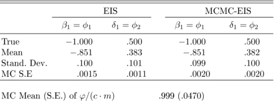
Table 5. Posterior Analysis of the AR(2) Model for Simulated Data EIS MCMC-EIS β1=φ1 δ1=φ2 β1=φ1 δ1=φ2 True −1.000 .500 −1.000 .500 Mean −.851 .383 −.851 .382 Stand. Dev. .100 .101 .099 .100 MC S.E .0015 .0011 .0020 .0020 MC Mean (S.E.) ofϕ/(c·m) .999 (.0470)
NOTE: The estimated model is given by Equation (41) withp= 2. The sample size for the simulated
data from that model isT= 100. The posterior moments are based on 5,500 parameter draws (discarding
the rst 500 draws). The EIS approximation to the likelihood`(φ;y)is based on 4 to 5 EIS iterations.
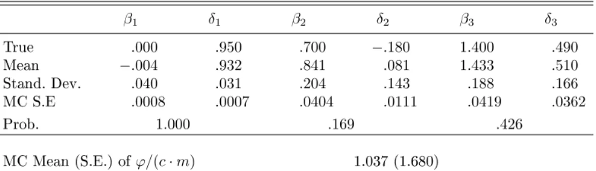
Table 6. MCMC-EIS Posterior Analysis of the AR(6) Model for Simulated Data β1 δ1 β2 δ2 β3 δ3 True .000 .950 .700 −.180 1.400 .490 Mean −.004 .932 .841 .081 1.433 .510 Stand. Dev. .040 .031 .204 .143 .188 .166 MC S.E .0008 .0007 .0404 .0111 .0419 .0362 Prob. 1.000 .169 .426 MC Mean (S.E.) ofϕ/(c·m) 1.037 (1.680)
NOTE: The estimated model is given by Equation (41) withp= 6and re-parameterized according to
(44). The sample size for the simulated data from that model isT = 100. The posterior moments are
based on 5,500 parameter draws (discarding the rst 500 draws). The EIS approximation to the likelihood `(φ;y)is based on 4 to 5 EIS iterations. The MC standard errors are based upon 100 replications of the
Fig. 1. Convergence of MC estimates of Ef(x)wheref is an inverse Gaussian distribution with kernel (30)
andθ1= 1.5 andθ2= 2. The exact value is 1.155. The nal estimates for a MC sample size 50,000 are
Fig. 2. Convergence of MC estimates ofEf(x2)wheref is a standardized student-t with density kernel (34)
andν = 2.5. The exact value is 1. The nal estimates for a MC sample size 50,000 are 0.4520 (MH-EIS),
Fig. 3. Convergence of MCMC posterior means for the SV parameters (left) and autocorrelation functions of the Gibbs draws of the parameters (right). The solid lines represent the results for the MCMC algorithm
based on the (single-block) EIS sampler forλand the dashed lines those for the corresponding single-move