Finding relevant videos in big data environments - how to utilize graph processing systems for video retrieval

Institute of Parallel and Distributed Systems University of Stuttgart

Universitätsstraße 38 D–70569 Stuttgart

Masterarbeit Nr. 123

Finding Relevant Videos in Big

Data Environments

-How to Utilize Graph Processing

Systems for Video Retrieval

Patrik Schäfer

Course of Study: Informatik

Examiner: Prof. Dr. rer. nat. Dr. h. c. Kurt Rothermel

Abstract

The fast growing amount of videos in the web arises new challenges. The first is to find relevant videos for specific queries. This can be addressed by Content Based Video Retrieval (CBVR), in which the video data is used to do retrieval. A second challenge is to perform such CBVR with big amounts of data. In this work both challenges are targeted by using a distributed Big Graph Processing System for CBVR. A graph framework for CBVR is built with Apache Giraph. The system is generic in regard of the used feature set. A similarity graph is built with the chosen features. The graph system provides a insert operation for adding new videos and a query operation for retrieval. The query uses a fast fuuzy search for seeds of a personalized Pagerank, which uses the locality of the similarity graph for improving the fuzzy search. The graph system is tested with SIFT features for object recognition and matching. In the evaluation the Stanford I2V is used.

Contents

1 Introduction 9

2 Content based video retrieval 11

2.1 How to compare videos? . . . 11

2.2 How to describe a video with features? . . . 11

3 Basic Ideas 15 3.1 Similarity Graph . . . 15

3.2 Insert and Query in the Similarity Graph . . . 16

3.3 Using the similarity graph for improving an initial search . . . 16

4 Big Graph Processing 19 4.1 Motivation . . . 19

4.2 Pregel . . . 20

4.3 Other Graph Systems . . . 25

5 Giraph 27 5.1 Block Framework . . . 27

5.2 YARN . . . 28

6 Graph System Implementation in Giraph 31 6.1 Generic Class Structure . . . 31

6.2 Computation Logic . . . 32

6.3 Dynamic Graph . . . 33

7 Features for object recognition 35 7.1 Feature selection . . . 35

7.2 SIFT . . . 36

7.3 Libraries . . . 39

7.4 Implementation of SIFT in the Generic Graph System . . . 40

8.2 Metrics . . . 44 8.3 Setup . . . 45 8.4 Results . . . 46

9 Summary and Outlook 49

Bibliography 51

List of Figures

2.1 Typical Video Retrieval System . . . 11

2.2 Segmentation . . . 12 4.1 Barrier Synchronization . . . 20 4.2 Vertex State . . . 22 4.3 Combiner . . . 23 5.1 Hadoop Evaluation . . . 28 5.2 Hadoop Architecture . . . 29 6.1 Generic Classes . . . 31

6.2 Block Flow Diagram . . . 32

7.1 Difficulties in Image Retrieval . . . 36

7.3 From keypoint to descriptor . . . 37

7.4 SIFT Matching . . . 38

1 Introduction

It has never been easier to make and distribute videos than today. The success of smartphones and tablets with integrated cameras makes it possible for almost everyone to make videos whenever wanted, because this devices accompany us in our everyday live. Advanced communication technology like LTE enables us to distribute our produced video in the internet from wherever we are. Through the Web 2.0 and Social Media, people want to share their content and there are a lot of platforms like YouTube or Facebook, which make it really easy to upload videos to the internet and share them with the community. 300 hours of video are uploaded to YouTube every minute [Rob14]. The Cisco VNI Forecast and Methodology, 2015-2020 states that "Globally, IP video traffic will be 82 percent of all consumer Internet traffic by 2020, up from 70 percent in 2015. Global IP video traffic will grow threefold from 2015 to 2020" and "It would take an individual more than 5 million years to watch the amount of video that will cross global IP networks each month in 2020" [Cis]. That’s a lot of video data and can make it difficult to find relevant videos in a query. Today’s common way to search for specific videos is via text search. The retrieval systems use annotated text in the meta data or surrounding text on a web page. To improve these searches, there is the idea to utilize the video content for retrieval. This leads to Content Based Video Retrieval (CBVR). With CBVR it is additionally possible to search videos, which contain a specific object of query image/video, which is hardly possible with text search. CBVR can improve the search, but through the fast growing amount of videos there is also a Big Data processing challenge. The CBVR system has to be able to process large amounts of data. Therefore a CBVR system is built, which uses a Framework, that is designed for Big Data processing.

The goal of this work is to provide a generic graph system, which is capable of processing a big similarity graph for video retrieval. The system is held generic in terms of features, because there are different recognition tasks and for each a broad spectrum of different features is existing. So it’s free for developers to adapt this graph system for his/her use case with the corresponding set of features. The graph system is built with Giraph, an open-source distributed graph-system for big graphs. To show that this approach can be useful in real world video retrieval tasks, a system, which uses SIFT features

1 Introduction

computation with which vertices are inserted in a similarity graph and a very cheap similarity computation for getting candidates for a query. The best candidates are used as seeds for some kind of personal Pagerank, which exploits the locality of the computed similarity graph to return good query results. This is done under the assumption that there are a lot more queries than inserts and therefore it’s worth to invest in building a similarity graph.

Structure

This work is structured in following way:

Chapter 2 – Content based video retrieval: In this chapter the fundamental func-tional principle of video retrieval is described.

Chapter 3 – Basic Ideas shows the approach for video retrieval proposed in this work. Chapter 4 – Big Graph Processing: In this chapter the ideas and functionality of graph

systems are presented.

Chapter 5 – Giraph: The characteristics of Giraph are shown.

Chapter 6 – Graph System Implementation in Giraph: The specific Giraph imple-mentation is roughly outlined

Chapter 7 – Features for object recognition: Possible features for CBVR are looked on and the SIFT descriptor and its implementation in the graph system is pictured. Chapter 8 – Evaluation: The functionality of the graph system is evaluated.

Chapter 9 – Summary and Outlook: The content of this work is summarized and a look in the future is taken.

2 Content based video retrieval

2.1 How to compare videos?

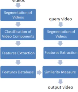
Figure 2.1: Features are extracted from the videos in the database as well as from the queried video. The features are compared and the results with the greatest similarity are returned. (Source: [AM15])

2.1 shows the process of video retrieval. During this process features have to be computed.

2.2 How to describe a video with features?

This question is highly dependent on what kind of videos should be compared to each other. If a video shall be checked in regard to whether it’s an near-duplicate or not, a

2 Content based video retrieval

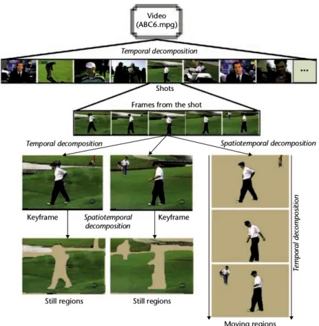
Figure 2.2: There are a lot of different segmentations of a video clip possible. The choice of the respective segmentation depends on the desired comparison objective. (Source: [BCGU10])

are a lot of different objects, scenes and actions in a video clip and it’s not a good idea to sample them in one single feature [AM15].

Here are some common steps how to segment a video: 1. Separate visual and audio data.

2. Segment the clip in so called shots. A shot is a part of the video clip where the scene remains the same and there are only little differences between two neighbored frames, e.g. a typical shot would be one camera angle with the shot boundary at a movie cut.

3. A shot can be segmented in different directions.

a) spatiotemporal: segment the moving object for action recognition features

2.2 How to describe a video with features?

b) temporal: Choose some descriptive frames from the shot and use classic image retrieval for object/scene recognition

4. Keyframes can be segmented further with segmentation techniques, which identify objects in the keyframe or by cutting out the moving object for better scene recognition

Shot detection and keyframe selection are a research field on their own and can become quite sophisticated [QLGW13][RN13].

Which segmentation is chosen depends on the intention of comparison. There also were attempts to combine different features like image features from keyframes, motion features and audio features, which are compared separately and a weighted similarity is built afterwards [BCGU10][YOH16]. The presented generic system can use all kinds of features and is able to combine different ones.

In the explicit use case of the graph system, the main focus is on object recognition. Therefore no spatiotemporal decomposition is done and the problem is reduced to compare keyframes to each other for which image descriptors are sufficient.

3 Basic Ideas

The generic framework, which was built in this work, supports two operations: insert and query. The insert operation adds a new object to the database and the query operation searches for the best matches of the queried item in the database. The system uses a similarity graph for this task.

3.1 Similarity Graph

The similarity graph built in this work is an undirected graph in which the edges are assigned the value of a similarity measure between the feature sets of two vertices. There is only an edge between two vertices if the similarity between them is above an user-defined threshold, so there are no low value edges.

In this work the graph is used to improve the result of a fast fuzzy search. The term fuzzy search is used for a search, which can be computed fast, but the results are not sufficiently precise and can be used as candidate set for better results. A example for a fuzzy search is the SIFT mean search (see Section 7.5 on page 41).

Such a graph could also be used for several other purposes like improving a previous text-based search or label propagation.

• Improving previous text-based searches:

There are a lot of existing search engines, that find relevant images/videos by using a text query which is matched with to images/videos attached text metadata. Other works have shown that visual similarity can be used to improve the search results of this conventional search [YOH16].

• Label Propagation:

Some videos (vertices) are labeled and the rest is not. The goal is to label all vertices. A similarity graph can used for this. A vertex gets the label assigned, which the most neighbors of the vertex had been assigned [WZ08].

3 Basic Ideas

3.2 Insert and Query in the Similarity Graph

• Insert: A new vertex shall be added to the graph. in order to build a perfect similarity graph, the features of the new vertex have to be compared to those of all existing other vertices. If the similarity to another vertex is above the predefined threshold-value an edge with the value of the similarity is generated. The comparison method for this is usually computational expensive. This method does not scale well when doing this for all inserted vertices, since the number of computations is quadratic in complexity. Thus the existing similarity graph is used for a more scalable heuristic insertion operation. The similarity graph provides a method to search for similar vertices, to which a potential edge would be created. The below described query operation is used to get potential candidates. The similarity is only computed to this set of candidates. The number of candidates is chosen a magnitude greater than the number of desired results of an eventual normal query operation, to be sure that there are barely edges not created, which should have been created.

• Query: The query is done by performing a fast fuzzy search to get seed nodes for the personal Pagerank, which uses the similarity graph to improve the fuzzy search (see in next section).

3.3 Using the similarity graph for improving an initial

search

The idea of using the similarity graph for improving a former search result is to exploit the locality of the similarity graph. Good results should have a high visual similarity and should have an edge and/or are close to other good results. Bad results should not have a high similarity to good results and should be more remote. If a vertex is near to many results, then it is probably a good result and is of relevance in this context. To exploit this locality, something like a personal Pagerank is computed. The top n results of the initial fuzzy search act as candidate set for seeds. For all candidates the SIFT matches are computed. If the number of matches is above a defined threshold, then the candidate is a seed. A seed is a vertex, which has a rank greater than zero as initial seed in the Pagerank. In this implementation all seeds get the value 1.0, but it is easily possible to weight the seeds in respect to the similarity to the query object. In standard Pagerank the random surfer has the probability (1 -α) to jump to one of its neighbours and the probability ofαto teleport to a random vertex. In this version the random surfer doesn’t teleport to a random vertex but instead he teleports to a seed vertex. This version of

3.3 Using the similarity graph for improving an initial search

Algorithmus 3.1Unweighted Personal Pagerank procedure VERTEXSEND(neighbors,rank)

for alledges∈neighborsdo send(_#neighborsrank )

end for end procedure

procedure VERTEXRECEIVE(messages,rank,initialRank)

sum←0

for allmessagesdo

sum←sum+value(message) end for

rank ←α∗InitialRank+ (1 +α)∗sum

end procedure

Pagerank can be seen as a generalization of random walkers which start at the seed vertices and walk along the edges in the graph with some probability to teleport back to the seed vertices instead. After computing some rounds of this Pagerank nearby seeds and common neighbors should have a better score than remote seeds.

Furthermore, the value of the edges can be used as well. More similar neighbours should get a greater amount of the rank of a node than less similar neighbors. Therefore, a weighted pagerank could provide the chance to perform better than an unweighted Pagerank.

4 Big Graph Processing

4.1 Motivation

At scale, everything breaks (Urs Hölzle, Google)

The quote of Urs Hölzle also applies to big graphs. Although there are powerful libraries, which perform very well on one machine, if the graph is big enough they are not sufficient anymore and a distributed solution is needed. It’s not very practical to craft a custom distributed infrastructure for different graph algorithms and representations. Thus an easy-to-use distributed framework with some fault tolerance mechanism would be desired. The well-informed reader will notice that this description sounds a lot like MapReduce. And rightly so: MapReduce is an easy-to-use distributed framework with some fault tolerance mechanism and a lot of algorithms are convertible in some way to fit in this framework, including a lot of graph algorithms. Unfortunately MapReduce is not well-suited for the most graph algorithms. In many cases it is not intuitive to express a graph algorithm as map()- and reduce() function. The transformation to these functions can be difficult to understand. Another problem is that a lot of graph algorithms rely on many iterations. A classical MapReduce job reads the data from a distributed file system, does the map- & reduce-step and stores the result back to the file system. It would be very time consuming to do this with a lot of iterations. Of course it is possible to stream MapReduce jobs without storing in between, but for a stream of hundreds of MapReduce steps it’s difficult to provide fault tolerance. That’s the reason why Google developed the Pregel System. Pregel is closed-source but Malewicz et al. published an article about the functionality of this system [MAB+10]. Because later graph systems are inspired by Pregel and Giraph implements the functionality of the Pregel paper one-to-one, the Pregel functionality is described in detail.

4 Big Graph Processing

4.2 Pregel

4.2.1 Bulk Synchronous Parallel

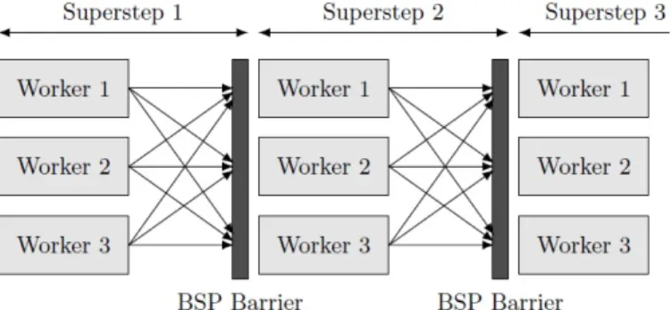
Figure 4.1: All workers need to wait until all other workers have finished the superstep. (Source: [KAA+13])

Pregel is inspired by the Bulk Synchronous Parallel (BSP) model, that was already presented in 1990 [Val90].

The BSP-model consists of three principles: 1. Parallel computation

- Each component can do local computations with locally stored data. 2. Communication

- Each component can communicate with other components and send them data.

3. Barrier Synchronization

- If some component reaches a certain point in computation (barrier), it waits for other components to also reach that point.

The barrier synchronization leads to so-called supersteps. In a superstep all components compute their data in parallel and communicate with each other. If all components finish their work and their communication, the next superstep can be started.

Pregel is vertex-centric which means that there is one compute() function, that each vertex can compute in parallel. The developer has to "think like a vertex", which should provide an easy pattern of thinking, so that it is possible to implement relatively complex algorithms with only a few lines of code.

4.2 Pregel

4.2.2 compute function

The compute()-function has the following properties during superstep s: • can receive messages from superstep s-1

• can send messages to other vertices, which are received at superstep s+1 • can change its value or the value of its outgoing edges

• can request to add/delete vertices or edges

4.2.3 Properties of vertices

Each vertex possesses • an unique identifier

• a mutable, user-defined value • a list of outgoing edges with each

– a mutable value

– an identifier of the target vertex • a halt flag

4.2.4 Setup

The input of Pregel is a directed graph in a (distributed) file system. The machines are called workers and one of them is the master. In superstep 0 the master partitions the graph and distributes the partitions to the workers. Per default the partitioning is solved with simple modulo arithmetic. A vertex with vertex-id i is mapped to the partition: i mod #partitions. The topology of the graph is hence not included. The master coordinates the supersteps, checks the workers for errors and holds the statistics of the current state of computation, e.g. the number of vertices. A worker holds its partitions in main memory, executes the compute()-functions of a partition in serial order and buffers outgoing messages to remote vertices.

4 Big Graph Processing

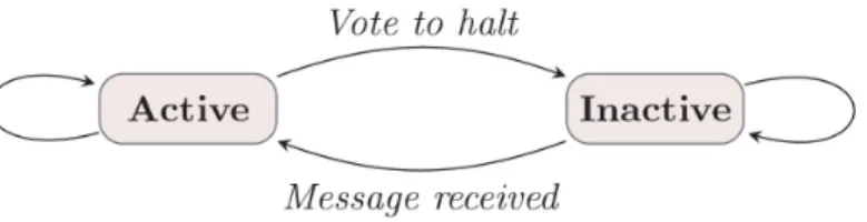
Figure 4.2: There are two states of a vertex: active or inactive. A vertex can vote to halt and becomes inactive until a message is received. (Source: [MAB+10])

4.2.5 Termination

At superstep 0 all vertices are active. In its compute()-function a vertex has got the opportunity to call the voteToHalt()-function. VoteToHalt() deactivates the vertex and sends a voteToHalt-message to the master. A deactivated vertex remains inactive and the compute()-function will not be scheduled until it is reactivated. If a deactivated vertex receives a message it changes its state to active and will be scheduled. The vertex then stays active until it calls the voteToHalt()-function again.

4.2.6 Messages

A message contains a value and the id of the target vertex. Typically messages are sent to neighbours, but this is not necessary. If a vertex knows other vertices, maybe through messages or through a public subset, it is possible to send messages to them, too. The underlying network protocol guarantees the delivery of messages, but makes no statement about the order the messages arrive.

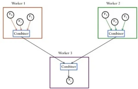
4.2.7 Combiner

The combiner enables the possibility to combine outgoing or incoming messages. The reduction of network traffic is an example use-case of this feature. Combiners can be applied if there is only the result of combined messages needed, e.g. the sum of the messages. The combination function has to be associative and commutative. In such a case it’s possible to build the combine of outgoing messages to the same vertex at the sending worker and instead of a lot messages only one combined message is sent. Incoming messages can also be combined in this way to speed up the compute()-function, because messages can be combined before the next superstep starts.

4.2 Pregel

Figure 4.3: Outgoing messages to the same worker can be combined to reduce traffic. Ingoing messages can also be combined, so the compute() method can be processed faster. (Source: [Zha])

4.2.8 Aggregators

Figure 4.4:Aggregators are used to collect global data (Source: [Zha])

Aggregators are used to collect global state or to enable something like a global commu-nication. E.g. its possible to count the number of edges and publish the result in the

4 Big Graph Processing

are some predefined aggregators like min, max and sum. Others can be written by the developer.

4.2.9 Topology changes

Topology changes can cause conflicts. For instance, one vertex sends a request to delete a certain vertex while another vertex sends a request for adding an edge to this vertex. To resolve such conflicts there is a default partial ordering in which sequence the requests will be executed.

1. delete edges 2. delete vertices 3. add vertices 4. add edges

In the scenario described earlier the vertex would be deleted and the edge request would be discarded. Other conflicts can not be resolved with this strategy, e.g. two different request to add a vertex with same id, but different value. For such a scenario the developer has to add a resolve strategy by himself if it is not wanted that the new vertex has randomly one of both values.

4.2.10 Fault tolerance

In order to make the system fault tolerant, it saves snapshots in regular intervals. The snapshot is taken between two supersteps. The workers save all vertices and outgoing edges including the value of their partition plus the incoming messages for their partition on persistent storage. The developer can specify the size of the interval, e.g. every 50 supersteps. To determine whether a worker has crashed, the master pings the workers periodically. If there is no reply the master assumes that the worker has crashed. The whole computation is reset to the last available snapshot. The graph is partitioned to the remaining workers. All computations since then are lost. To avoid the loss of already computed results, the original paper suggests a limited recovery, however this was not tested in practice. The idea of this approach is that the workers store their outgoing messages since the last snapshot. In case of failure the partition of the failed worker can use the messages to recover. The other workers don’t have to recompute. This strategy needs the graph algorithm to be deterministic, because the state of the recovered partition has to match with the other partitions.

4.3 Other Graph Systems

4.3 Other Graph Systems

After the Pregel paper was published, other distributed Big Graph Systems emerged. Some popular examples:

• Giraph: described in detail in Chapter 5.

• PowerGraph [GLG+12]: Does a vertex cut instead of a edge cut for better load balancing and uses a scatter-gather approach instead of the vertex compute(). It provides the possibility to soften the BSP model with asynchronous computation using a locking mechanism.

• GraphX [XGFS13]: Is part of the Apache Spark project and provides a Pregel API for graph computation. The embedding in Spark and the use of RDFs make it easy to compose a graph computation with e.g. a MapReduce task and another graph computation.

• GPS [SW13]: Additionally to the Pregel functionality GPS proposed dynamic repartitioning of the vertices to minimize network traffic.

In this work I chose to use Giraph, because the overall package seemed to fit the best: • It is open-source.

• It is popular since it is still under development, used by a big community and therefore it is well documented.

• It provides graph mutations.

5 Giraph

Apache Giraph is an open-source implementation of the system described in the Pregel paper [Ave11]. It’s an Apache top level project and is under steady development. It is for example used by Facebook for analyzing their social graph and by Yahoo. It uses Apache Hadoop YARN (see Section 5.2) for resource management and Apache Zookeeper [HKJR10] for synchronization of the supersteps. It is implemented in Java. In addition to the Pregel functionality it provides some extensions like master computation, out-of-core computation, sharded aggregators, edge-oriented input and composable computation. The master computation allows to do some global computation between two supersteps and provides the possibility to broadcast data to the workers.

5.1 Block Framework

The Block Framework is a new API for Giraph applications. Internally the Block Frame-work relies on the normal Pregel/Giraph API with supersteps. Instead of having a compute()-method, which determines the vertex computation in one superstep and the mastercompute() between the supersteps, there are pieces that each consist of a sending phase, the mastercompute() and a following receiving phase. A piece is an atomic block. It’s possible to compose multiple pieces to a more complex block. The separation between sending and receiving is only logical. Internally the receiving phase of one block and the sending of the next block are processed in the same superstep. The new API is introduced to improve the encapsulation and make it easier to implement complex algorithms with different computation phases [15]. Up to now, if there were different conditional computations, the developer had to place them in the compute() method with some conditional switch depending on the number of supersteps or an aggregator value. The message format had to be always the same.

The Block Framework changes this. Different phases of the computation can be imple-mented in different blocks. Blocks can be composed in various ways, such as

5 Giraph

• RepeatBlock: The block is processed for the stated value of iterations times. • RepeatUntilBlock: The block is repeated until the Boolean value changes to true. Data can be transferred between adjacent blocks with ObjectTransfer objects. For example, if the next block needs the results of the former and the results aren’t stored in the vertex value.

The advantage of this approach is that the computation is cleanly separated and it’s easier to model a changing algorithm or consecutive algorithms with it. For example Pagerank could be built with a RepeatBlock of an iteration piece with a number of iterations specified. A more complex example can be found at Section 6.2.

5.2 YARN

Figure 5.1: An additional layer is added to separate the resource management from the computation model.(Source: [14])

The initial Giraph used the Hadoop MapReduce Framework [SKRC10] for pushing its code to the given compute resources. It was a so called map-only application, which didn’t make use of the MapReduce paradigm and was cut off from the Hadoop data pipelines. The use of Hadoop was the resource management and the functionality to schedule the Giraph tasks at the available resources.

Because there were other applications, which used Hadoop without doing a usual MapRe-duce and some other reasons like scalability YARN (Yet Another Resource Negotiator) was created [VSS+13]. YARN decouples the programming model from the resource management.

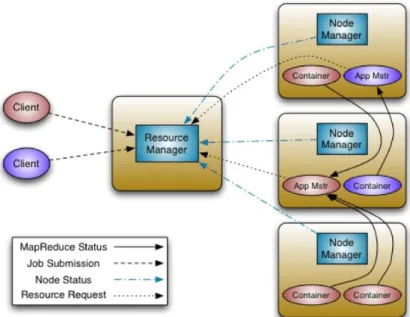
The dedicated Resource Manager (RM) has got a global view of all resources and is responsible for allocating these resources, so-called containers. It obtains its global view

5.2 YARN

Figure 5.2: The Resource Manager starts the Application Master, which is aware of com-putation requirements and requests containers from the RM and manages them. (Source: [Mur])

from NodeManagers which run on all nodes, communicate with the RM and allocate the local resources if the RM commands it. It also accepts new jobs by allocating a container for the ApplicationManager(AM). The AM coordinates the programming logic of the job and requests resources from the RM. The RM doesn’t know the semantics of the requested resources.

6 Graph System Implementation in

Giraph

6.1 Generic Class Structure

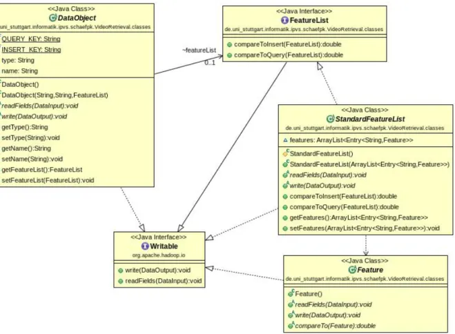
Figure 6.1:Generic Classes

6 Graph System Implementation in Giraph

Figure 7.5 shows the generic class diagram which can be specialized for different sets of features and comparison methods.

The input of the video retrieval system are DataObjects, which consist of a type, a name and a feature list. The type is either QUERY or INSERT. The name is a string, which can be used to identify the object. The FeatureList has got two methods "compareToQuery" and "compareToInsert" which have to be implemented by the developer. "compareTo-Query" should be a fast computation to get an approximation and "compareToInsert" a computation heavy operation to get the edge values. The developer has to ensure that FeatureLists and Features are compared to the same kind of FeatureList/Feature. All classes have to implement the org.apache.hadoop.io.Writable interface, so they can be used in Giraph.

6.2 Computation Logic

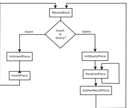
Figure 6.2: Block Flow Diagram

The developed graph system for video retrieval was built using the Block Framework of Giraph, described in Section 5.1. Figure 6.2 shows the flowchart of the execution order of the different blocks. First, the next object (or objects) to insert or query is read in the MasterBlock. The type of read object(s) determines which branch is taken. If more than one object should be processed as batch, the objects have to be either all "insert" or all "query". The data object provider has to ensure that only requests of the same type are bundled. If it is a query object, the left branch is taken and the next Block is

6.3 Dynamic Graph

the InitPiece. If it is an object to insert, the InsertInitPiece is executed. The MasterBlock publishes the read data object to the workers.

The InsertInitPiece performs a query to find candidates for which an edge should be created. In the InsertPiece a new vertex is added and all candidates compute their similarity to the the new vertex. If the similarity is above the user-defined threshold, an edge from the candidate to the new vertex, as well as from the new vertex to the candidate is created.

The query branch consists of several blocks. The first block is the InitPiece. Here, all vertices compute the fast "compareToQuery" method, which will give an approximate similarity. The computed results will be reduced within a priority queue, so the master knows the top n distances. These will be broadcast back to the workers and the top n vertices are matched against the query data object and if there are enough matches, they are set to an initial rank greater than zero for the following personal Pagerank. The next block is the iteration block, which represents basically one iteration of the algorithm described in Algorithm 3.1.

There are two different possible implementations of this block. Either it runs a fixed number of iterations or it runs until the Pagerank converges. After the iterations reached their maximum or the Pagerank has converged the GatherResultBlock is executed. Like in the InitPiece the top n ranks of the Pagerank are reduced to the master with a priority queue. After this the whole loop starts again with the MasterBlock reading a new data object.

6.3 Dynamic Graph

The primary purpose of Giraph is to compute on a premade graph. Giraph indeed allows graph mutations, but these are rather designed to modify an existing graph, e.g. add shortcuts or delete edges in the course of an algorithm. On account of this, the API of the mastercompute() doesn’t have the possibility to send a request to create a vertex. Instead all graph mutations are requested in vertexcompute(). Because all vertices execute the same vertexcompute() there has to be a mechanism to prevent a lot of identical vertex requests. This is solved by a special vertex, which is determined by its id and is responsible to send vertex requests. The data objects read by the MasterBlock are provided by a DataProvider class, which’s implementation is not fixed. In the evaluation example the data objects are stored in a file on the Hadoop file system and the provider delivers them to the MasterBlock.

7 Features for object recognition

7.1 Feature selection

A lot of research has been done and is yet ongoing in terms of image comparison and retrieval.

Hence, there is a broad spectrum of feature descriptors for image retrieval available. There are two main groups of descriptors: global and local descriptors.

7.1.1 Global descriptors

Global features describe an image/object as a whole. They describe an object with just a single vector, but they are not able to distinguish between background and foreground. There are color descriptors and texture descriptors.

• Color descriptors: Color is one of the most important properties for human image comparison. One of the most used color descriptors is the color histogram, which describes the color distribution in the whole image (e.g. MPEG7 CSD [Sik01]). • Texture descriptors: Textures are characteristic, repetitive patterns in a certain

relation, which makes it easy for humans to recognize an object, e.g. leaves or waves. One example for a texture descriptor is the MPEG 7 Edge Histogram Descriptor [Sik01], which categorizes the edges into 5 bins according to their direction.

Creating global descriptors for an entire image is useful, if the overall composition is interesting for image comparison.

To increase the usefulness for object recognition, a preceding segmentation step can be used. A segmentation can be obtained by motion information of a video for example. Without such additional information or a clean background, segmentation is challenging

7 Features for object recognition

7.1.2 Local descriptors

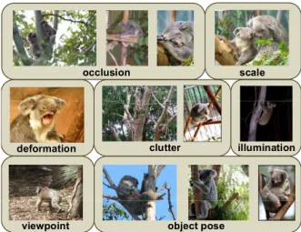
Figure 7.1: There are a lot of varieties in which an object can appear on an image, which makes object recognition quite hard. (Source: [TM07])

To obtain local descriptors, an image is searched for interesting points, so called key-points. The number of detected keypoints varies, because some images can have more interesting points than others. After finding the keypoints, there must be a region defined around the keypoint which should be distinctive and preferably scale- or affine invariant. This region has to be normalized and is put in a descriptor vector that is highly expressive and good for matching. In terms of object recognition and matching, local features have shown to be more robust against image clutter and occlusion [AFS93][TM07].

The most noted state-of-art descriptors are SIFT [Low04] and SURF [BETV08], which are both patented and not free for use. There are a lot more used and competitive descriptors like ORB [RRKB11], BRIEF [LCS11], BRISK [LCS11] and derivatives of SIFT like PCA-SIFT [KS04] or ASIFT [MY09].

I decided to use SIFT. Although this descriptor is existing for more than ten years, it is still very often the benchmark for newly developed descriptors [TM07].

7.2 SIFT

SIFT stands for Scale-Invariant Feature Transform.

SIFT features are fixed length vectors. In practice they have 128 dimensions. Each dimension needs one byte to store, thus a SIFT feature needs 128 byte to store. Like other local descriptors, the SIFT algorithm searches an image for keypoints and the

7.2 SIFT

Figure 7.2: Different octaves with different blurs. The Difference of Gaussians are the differences between two differently blurred images of the same octave. (Source: [TM07])

number of generated features for a given image varies. To achieve scale invariance, the algorithm constructs a scale space. The size of an image is internally halved several times. The different sizes are called octaves. Additionally, the images of the octaves are blurred with the Gaussian Blur several times. This is done in order to compute the Difference of Gaussians (DoG), which are simply the differences between two different blurred images of the same size. The DoG approximates the Laplacian of Gaussian, which reduces random noise and sharpens the edges of the image. For finding keypoints the maxima and minima in the DoGs are located. A pixel is a maximum/minimum, if its the greatest or smallest of all its neighbors. The neighbors are the eight pixels around the pixel plus the nine pixels at the same location at the one less blurred DoG image plus the 9 pixels at the one more blurred DoG image. Keypoints in low contrast environments and keypoints on edges are rejected, since the algorithm is more interested in corners.

7 Features for object recognition

For achieving rotation invariance, the keypoints need an orientation. To assign orien-tations to keypoints, the gradient directions and magnitude of the neighborhood are used to build a histogram. The biggest peak of the histogram is the orientation which is assigned. If there are peaks with at least 80% of the biggest peak, new keypoints are created for them.

To store the determined keypoints and in order to be able to compare them, a represen-tation is needed. First a 16x16 window around the keypoints is created. This window is divided in 4x4 blocks. For each of this block a 8 bin orientation histogram is created. This results in 4x4x16 = 128 numbers, which build the SIFT feature vector. The vector is normalized to numbers between 0 and 512, so each dimension can be stored within one byte.

7.2.1 Matching

Figure 7.4: This example shows the importance of geometric validation with RANSAC to get rid of false matches. (Source: [AFS93])

7.3 Libraries

For matching a set of SIFT features to another set of SIFT features, the nearest neighbors in the other set have to be found. It’s difficult to find an exact solution for this problem in high dimensional spaces with an acceptable runtime. Beis & Lowe proposed the Best Bin First-Algorithm, which is a variation of the k-d-tree search [BL97]. The kd-tree is build in the way that the space is always split in the dimension with the highest variance. The idea of this algorithm is that the bins in high density regions are smaller and thus, it is probable that the nearest neighbor of the queried point is in the leaf bin, where the search ends. If it is not in that bin, there is a high probability that the nearest neighbor is in an adjacent bin. Therefore, the distance to the up to now found nearest neighbor can be stored and a backtracking in the k-d-tree is performed. Bins which are not in the radius of the stored distance can be pruned. This performs well for low dimensions, but if there is a high-dimensional space, it’s not very effective because there are a lot of adjacent bins which can’t be pruned. Beis & Lowe observed, that bins with higher distances to the query point are unlikely to contribute the nearest neighbor, because the nearest neighbour would have to be in a small segment of the whole bin. To exploit this property only a fixed number of the nearest bins are scanned, which leads to a good approximation. To be able to do so, in the backtracking process a priority queue with the distances of not taken branches is built and stored. After a bin is evaluated, the branch of the tree is taken, which has the lowest distance to the query until the fixed number is reached.

Lowe suggests to consider a match a good match, if the distance to the nearest neighbor is smaller than 0.8 times the distance to the second nearest neighbor.

Unfortunately there are still a lot of false matches. In order to reduce them, it is possible to add an additional filter step. Correct matches should be part of a geometric (e.g. an affine) transformation from one image to the other. For learning a good transformation matrix, RANSAC is used [FB81]. The RANSAC algorithm takes a sample of matches with which it computes a model. After that, it tests all other matches, if they satisfy the model (inlier) or not. This will be iterated several times and the transformation with the most inliers is the output. Matches, which are not inliers of the final transformation, are discarded.

7.3 Libraries

There are different libraries for SIFT descriptor extraction and matching. Because Giraph is built in Java, Java libraries were tested in this work.

7 Features for object recognition

But tests showed that OpenCV, which is native in C/C++, but has got a Java interface, outperforms the OpenIMAJ implementation in SIFT matching. OpenCV uses the further developed FLANN [ML09][ML14] matcher for initial matches. Whether the FLANN matching process is faster or the implementation is more efficient was not determined, but the overall time for matching was notably faster. Therefore, I used OpenCV in this work.

7.4 Implementation of SIFT in the Generic Graph System

Figure 7.5:Implementation of SIFT features in the Graph System

7.5 SIFT Mean for fuzzy search

In this work the approach is tested with SIFT features. Therefore, a SIFTDataObject and a SIFTFeatureList with the features SIFTListFeature and SIFTMeanFeature are derived from the abstract classes as described in Section 6.1. The SIFTListFeature contains a list of the 128 dimensional sift vectors and the SIFTMeanFeature contains one vector, which is the mean of all SIFT features of the SIFTListFeature. The "compareTo" method of the SIFTListFeature is the in Section 7.3 mentioned FLANN matching for SIFT features. The "compareTo" of the SIFTMeanFeature is simply the Euclidean Distance between the two vectors of two different SIFTMeanFeatures. The "compareToQuery" method uses the "compareTo" method of the SIFTMeanFeature and the "compareToInsert" method uses the "compareTo" method of the SIFTFeatureList.

7.5 SIFT Mean for fuzzy search

Anh, Nam, Hoang, et al. proposed the idea to condense all SIFT descriptors of one object in a single mean vector, which contains in each of its dimension the mean of all SIFT descriptors in this dimension [ANH+10]. They showed that objects with a lot of SIFT matches are likely to have a lesser Euclidean Distance between the mean vectors than objects, which have a greater distance between the mean vectors. This observation can be used to get a fast candidate set. Other works are also using SIFT mean vectors for candidates [LA16][ABK+12].

8 Evaluation

8.1 Stanford I2V

Standford I2V [ACC+15] is a video database, which addresses the problem of querying a video database with images. It provides 3,800 hours of newscast videos and annotated more than 200 ground-truth queries with a benchmark for retrieval. 8.1 shows example query images with frames of videos which are relevant for this query image.

8 Evaluation

8.2 Metrics

The video retrieval graph system returns an ordered list of n results. A result is either relevant or not relevant.

8.2.1 Mean Average Precision

The usual metrics for retrieval tasks are precision and recall.

Precision= Number of relevant items retrieved Total number of items retrieved

Recall= Number of relevant items retrieved Total number of relevant items

Precision and recall alone aren’t a good metric for evaluating a fixed number of ranked results. What if the number of relevant items is smaller than n and all relevant items are first in the returned list and rest of the list is filled with irrelevant videos, because there were no more relevant videos. The recall would be 1, but the precision would be less than 1, because of the filling with irrelevant videos. Or in another case, where the number of relevant items would be greater than n and the result list consists only of relevant items. The precision would be 1, but the recall would be less than 1, because there exist relevant items, which were not returned. In both scenarios the system returned the best possible result and it would be desired that in both scenarios the system gets a perfect score. Additionally this metrics are not sensitive to the ranking of the n items. Precision and recall would be the same, if the relevant results are in front of the ordered list or at the end. Therefore the mean average precision (MAP) is used for evaluation in this work. This metric is also used in the I2V dataset benchmark and a lot of different video retrievals [DKN08][CMD+05][SOK06]. First the average precision for each query is calculated:

MAP= NR X i=1

Precision(Recalli),

whereNR is the total number of relevant items and i is the i-st relevant item in the list and Precision(Recalli)will be defined as

Precision(Recalli) = Number of relevant items until rank(i)

i

8.3 Setup

,

where rank(i) is the position of the i-st in the ordered list. The MAP is only computed for the relevant items in the result set.

Here is an example: N =5 The first returned item is relevant, the second is not, the third is relevant, the fourth is not relevant and the fifth is relevant again. Thus NRis 3. Precision(Recall1) = 1, Precision(Recall2) = 2₃, Precision(Recall3) = 3₅

Average Precision(R)= 1 + 2 3 + 2 3 3 ≈0.76

Assuming we switch the first with the second item, so that the first is irrelevant and second is relevant: Average Precision(R)= 1 2 + 2 3 + 2 3 3 ≈0.59

One can see, that this metric is sensitive to the ranking and in the scenarios described above, the AP would be 1.0.

The average precision is computed for all queries and the mean of it is calculated:

qMAP= 1 Q Q X q=1 Average Precision (q),

where Q is then number of queries.

8.3 Setup

Giraph is used in the version 1.2 and is compiled for pure YARN. Hadoop is used in the version 3.0.0-alpha. The evaluation is run on a cluster of 6 virtual OpenStack machines with 4 cores and 32GB RAM each. 16 workers are distributed over the 6 machines. Each work has a GiraphYarnHeap of 8GB. With the application master and the the master compute there are 18 containers running on YARN. To keep it simple, keyframes are taken at each second of the used I2V videos. The number of Pagerank iterations was 10. The threshold for creating an edge was 100 matches after RANSAC. This resulted in a sparse graph with just 0,5% edges created of all possible edges. Candidates are seeds if

8 Evaluation

8.4 Results

The first thing to mention is the size of the SIFT descriptors for the keyframes. Because all descriptors are in the vertex value they are loaded in main memory. For all the keyframes from the Stanford I2V there are between 300 and 5000 descriptors. To imagine the data size binary stored descriptors for 25000 keyframes have a size of more than 6GB. For this reason only a small subset of I2V dataset is used to test the system. For future work it could be worthwhile to use smaller descriptors (some are mentioned in Section 7.1.2) to reduce the memory consumption.

8.4.1 Insert

The first discovery, which was made, was that it’s not feasible to compute the SIFT matches (see Section 7.2.1) of each vertex pair to create the edges. The computation of SIFT matches is too expensive and even for small examples the quadratic complexity leads to extreme long runtime. Therefore a heuristic had to be found. The system is able to do queries and so it is intuitive, that performing a query gives a sufficiently good candidate set for which the exact matches can be computed.

In the earlier versions of the graph system, only one vertex was inserted per insert operation. An insert operation needs several supersteps: Reading the data object in the MasterBlock, getting the candidate set with the InitInsertPiece and subsequent computation of exact matches for the candidate set. It showed that this is not efficient for one single vertex, because the communication and synchronization effort is too high and it’s better to insert a batch of vertices:

Figure 8.2: Mean time for a vertex insert in relation to the batch size

Figure 8.2 shows that a good batch size is 100. A greater batch size doesn’t yield an improvement as the average throughput decreases slightly.

8.4 Results

Metric Fuzzy Search Query Result Keyframes Average Precision 0.09 0.21 qMAP 0.22 0.71 Clips Average Precision 0.21 0.30 Average Recall 0.46 0.78 qMAP 0,38 0,85

Table 8.1: Results of the retrieval

8.4.2 Query

Likewise, it is a good idea in terms of efficiency to run more than one query in parallel, because of the synchronization/communication effort. A personal Pagerank for several queries with ten iterations can be computed in 60 seconds.

The size of the candidate set (results of the fuzzy search) had to be larger than expected, because if chosen too small, for some queries no single relevant (enough matches) candidate is returned. With no relevant candidates the Pagerank has no seeds. Tests have shown that the candidate set should be in the size of 5% of the overall vertex number. Maybe the SIFT mean heuristic would work better, if the SIFT descriptors are not extracted for whole images but rather for individual objects after an image segmentation.

The retrieval is evaluated on two levels: The keyframe level and the clip level. In the keyframes level it is evaluated how good the precision is if the result list contains relevant and irrelevant keyframes. When watching Table 8.1 it has to be taken into account, that the average Precision is the ranking insensitive precision in relation to n and the qMAP is the ranking sensitive mean average precision in relation to the recall. At the clip level the result list contains clips instead of keyframes.

As in Section 8.2.1 mentioned, the Precision without relation to the recall is not meaning-ful, because in general n (the size of the results) is greater than the number of relevant results. As seen in Table 8.1 the personalized Pagerank in the similarity graph improves the results of the fuzzy search significantly. Specially the qMAP has a big impact on the quality of the results. The validation makes sure that the seeds are likely to be relevant, so the first results of vertices which are seeds themselves or vertices near them are good results. Unfortunately, the results are not comparable with the benchmark of the I2V

8 Evaluation

It showed that there is no need for a lot of Pagerank iterations. 10 or even less are sufficient for good results. Additional tests have shown that it is possible to reduce the number of messages by setting a threshold for the rank value of a vertex. If the rank of a vertex is below the threshold the vertex doesn’t spread its rank to its neighbors. If chosen small (0.1 still showed reasonably good results), this restriction does not effect the quality of the results.

9 Summary and Outlook

To adress the growing number of videos and the resulting challenges of doing Content Based Video Retrieval in a Big Data environment, this work proposes an approach to do CBVR with a Big Graph Processing System. For CBVR features have to be extracted of the video data, in order to be able to do matching. A generic graph system was built with Apache Giraph to support CBVR for an arbitrary set of features. Giraph is a popular distributed Big Graph Processing System, which is able to do distributed computations on big graphs. The graph system uses a similarity graph to do a personalized Pagerank. To get candidates for seeds of the Pagerank a fast fuzzy search is performed. The system was tested with SIFT descriptors as features. For the fast fuzzy search the SIFT descriptors of a keyframe are composed in one mean vector, which is matched by Euclidean Distance. The evaluation showed that the big data size of the SIFT descriptors is a problem in terms of scalability. The personalized Pagerank with seeds in the similarity graph provides a significant improvement of the fuzzy search. Maybe a similiar system with more light weight descriptors provides comparably good query results with less required memory. The personal Pagerank is a highly local computation, especially if the spread is limited by a threshold. Tests showed that the results don’t get worse if a small enough threshold is applied. The locality can be exploited by better partitioning. Near vertices should be in the same partition. There are systems [SW13][MTLR16], which are able to do such dynamic repartitioning to reduce network traffic, which can be an improvement to the existing system. In my estimation, the growing importance of video retrieval and the vast variety of feature extraction methods will lead to a lot of scientific progress in video retrieval in future years.

Bibliography

[14] How YARN Overcomes MapReduce Limitations in Hadoop 2.0. 2014. URL:

http : / / saphanatutorial . com / how yarn overcomes mapreduce -limitations-in-hadoop-2-0/(cit. on p. 28).

[15] Introducing Blocks Framework for Giraph. 2015. URL:http://mail-archives.

apache . org / mod _ mbox / giraph dev / 201506 . mbox / %3CCABJ n3v -24YLzgNmrT3TZT6R8t4Vw1hrBcWWTghG _ XgaC % 3DYqrg % 40mail . gmail.com%3E(visited on 01/25/2017) (cit. on p. 27).

[16] A comparison of state-of-the-art graph processing systems. 2016. URL:https: //code.facebook.com/posts/319004238457019/a-comparison-of-state-of-the-art-graph-processing-systems/ (visited on 01/18/2017) (cit. on p. 25).

[ABK+12] T. Q. Anh, P. Bao, T. T. Khanh, B. N. Da Thao, T. A. Tuan, N. T. Nhut. “Video Retrieval using Histogram and Sift Combined with Graph-based Image Seg-mentation.” In:Journal of Computer Science8.6 (2012), p. 853.URL:http:// search.proquest.com/openview/034fc7ae091c15571c8febb772204b4e/ 1?pq-origsite=gscholar&cbl=1216344(visited on 01/17/2017) (cit. on p. 41).

[ACC+15] A. Araujo, J. Chaves, D. Chen, R. Angst, B. Girod. “Stanford I2V: a news video dataset for query-by-image experiments.” en. In: ACM Press, 2015, pp. 237–242.ISBN: 978-1-4503-3351-1.DOI:10.1145/2713168.2713197.

URL:http://dl.acm.org/citation.cfm?doid=2713168.2713197(visited on

01/18/2017) (cit. on p. 43).

[AFS93] R. Agrawal, C. Faloutsos, A. Swami. “Efficient similarity search in sequence databases.” In: International Conference on Foundations of Data Organiza-tion and Algorithms. Springer, 1993, pp. 69–84.URL:http://link.springer. com/chapter/10.1007/3-540-57301-1_5(visited on 01/18/2017) (cit. on pp. 35–38).

Bibliography

[AM15] A. Ansari, M. H. Mohammed. “Content based Video Retrieval Systems-Methods, Techniques, Trends and Challenges.” In: International Journal of Computer Applications 112.7 (2015). URL: http : / / search . proquest . com/openview/6150ece2f051ecea27b68530e0bb9fd5/1?pq-origsite= gscholar (visited on 01/18/2017) (cit. on pp. 11, 12).

[ANH+10] N. D. Anh, B. N. Nam, N. H. Hoang, et al. “A new CBIR system using sift combined with neural network and graph-based segmentation.” In: Asian Conference on Intelligent Information and Database Systems. Springer, 2010, pp. 294–301. URL: http://link.springer.com/chapter/10.1007/978-3-642-12145-6_30(visited on 01/17/2017) (cit. on p. 41).

[Ave11] C. Avery. “Giraph: Large-scale graph processing infrastructure on hadoop.” In: Proceedings of the Hadoop Summit. Santa Clara 11 (2011) (cit. on p. 27).

[BCGU10] M. Bastan, H. Cam, U. Gudukbay, O. Ulusoy. “Bilvideo-7: an MPEG-7-compatible video indexing and retrieval system.” In:IEEE MultiMedia17.3 (2010), pp. 62–73. URL: http://ieeexplore.ieee.org/xpls/abs_all.jsp?

arnumber=5692184(visited on 01/18/2017) (cit. on pp. 12, 13).

[BETV08] H. Bay, A. Ess, T. Tuytelaars, L. Van Gool. “Speeded-up robust features (SURF).” In: Computer vision and image understanding 110.3 (2008), pp. 346–359 (cit. on p. 36).

[BL97] J. S. Beis, D. G. Lowe. “Shape indexing using approximate nearest-neighbour search in high-dimensional spaces.” In: Computer Vision and Pattern Recognition, 1997. Proceedings., 1997 IEEE Computer Society Confer-ence on. IEEE, 1997, pp. 1000–1006. URL:http://ieeexplore.ieee.org/xpls/

abs_all.jsp?arnumber=609451(visited on 01/17/2017) (cit. on p. 39). [CEK+15] A. Ching, S. Edunov, M. Kabiljo, D. Logothetis, S. Muthukrishnan. “One

trillion edges: graph processing at Facebook-scale.” In:Proceedings of the VLDB Endowment8.12 (2015), pp. 1804–1815. URL:http://dl.acm.org/

citation.cfm?id=2824077 (visited on 01/18/2017) (cit. on p. 25). [Cis] V. Cisco.Forecast and Methodology, 2015-2020(cit. on p. 9).

[CMD+05] P. Clough, H. Müller, T. Deselaers, M. Grubinger, T. M. Lehmann, J. Jensen, W. Hersh. “The CLEF 2005 cross–language image retrieval track.” In:

Workshop of the Cross-Language Evaluation Forum for European Languages. Springer, 2005, pp. 535–557 (cit. on p. 44).

Bibliography

[DKN08] T. Deselaers, D. Keysers, H. Ney. “Features for image retrieval: an experi-mental comparison.” en. In:Information Retrieval11.2 (Apr. 2008), pp. 77– 107. ISSN: 1386-4564, 1573-7659. DOI: 10.1007/s10791- 007- 9039- 3.

URL:http://link.springer.com/10.1007/s10791-007-9039-3(visited on

01/17/2017) (cit. on p. 44).

[FB81] M. A. Fischler, R. C. Bolles. “Random sample consensus: a paradigm for model fitting with applications to image analysis and automated cartog-raphy.” In: Communications of the ACM 24.6 (1981), pp. 381–395.URL:

http://dl.acm.org/citation.cfm?id=358692 (visited on 01/28/2017) (cit. on p. 39).

[GLG+12] J. E. Gonzalez, Y. Low, H. Gu, D. Bickson, C. Guestrin. “PowerGraph: Dis-tributed Graph-parallel Computation on Natural Graphs.” In:Proceedings of the 10th USENIX Conference on Operating Systems Design and Implemen-tation. OSDI’12. Berkeley, CA, USA: USENIX Association, 2012, pp. 17–30.

ISBN: 978-1-931971-96-6. URL: http : / / dl . acm . org / citation . cfm ? id = 2387880.2387883(cit. on p. 25).

[HDA+14] M. Han, K. Daudjee, K. Ammar, M. T. Özsu, X. Wang, T. Jin. “An Exper-imental Comparison of Pregel-like Graph Processing Systems.” In: Proc. VLDB Endow. 7.12 (Aug. 2014), pp. 1047–1058. ISSN: 2150-8097. DOI:

10.14778/2732977.2732980.URL:http://dx.doi.org/10.14778/2732977.

2732980(cit. on p. 25).

[HKJR10] P. Hunt, M. Konar, F. P. Junqueira, B. Reed. “ZooKeeper: Wait-free Coor-dination for Internet-scale Systems.” In: Proceedings of the 2010 USENIX Conference on USENIX Annual Technical Conference. USENIXATC’10. Berke-ley, CA, USA: USENIX Association, 2010, pp. 11–11. URL:http://dl.acm.

org/citation.cfm?id=1855840.1855851(cit. on p. 27).

[KAA+13] Z. Khayyat, K. Awara, A. Alonazi, H. Jamjoom, D. Williams, P. Kalnis. “Mizan: A System for Dynamic Load Balancing in Large-scale Graph Pro-cessing.” In: Proceedings of the 8th ACM European Conference on Com-puter Systems. EuroSys ’13. New York, NY, USA: ACM, 2013, pp. 169– 182. ISBN: 978-1-4503-1994-2. DOI: 10.1145/2465351.2465369. URL:

http://doi.acm.org/10.1145/2465351.2465369 (cit. on p. 20).

[KS04] Y. Ke, R. Sukthankar. “PCA-SIFT: A more distinctive representation for local image descriptors.” In:Computer Vision and Pattern Recognition, 2004. CVPR 2004. Proceedings of the 2004 IEEE Computer Society Conference on. Vol. 2. IEEE, 2004, pp. II–II (cit. on p. 36).

Bibliography

[LA16] H. Lacheheb, S. Aouat. “SIMIR: New mean SIFT color multi-clustering image retrieval.” en. In: Multimedia Tools and Applications (Feb. 2016).

ISSN: 1380-7501, 1573-7721. DOI:10.1007/s11042-015-3167-3. URL:

http : / / link . springer. com / 10 . 1007 / s11042 - 015 - 3167 - 3 (visited on 01/17/2017) (cit. on p. 41).

[LCS11] S. Leutenegger, M. Chli, R. Y. Siegwart. “BRISK: Binary robust invariant scalable keypoints.” In:Computer Vision (ICCV), 2011 IEEE International Conference on. IEEE, 2011, pp. 2548–2555 (cit. on p. 36).

[LLHY07] L. Liu, W. Lai, X.-S. Hua, S.-Q. Yang. “Video histogram: A novel video signature for efficient web video duplicate detection.” In: International Conference on Multimedia Modeling. Springer, 2007, pp. 94–103. URL:

http://link.springer.com/chapter/10.1007/978- 3- 540- 69429- 8_10

(visited on 01/19/2017) (cit. on p. 11).

[Low04] D. G. Lowe. “Distinctive image features from scale-invariant keypoints.” In:International journal of computer vision60.2 (2004), pp. 91–110.URL:

http://link.springer.com/article/10.1023/B:VISI.0000029664.99615.94

(visited on 01/17/2017) (cit. on p. 36).

[MAB+10] G. Malewicz, M. H. Austern, A. J. Bik, J. C. Dehnert, I. Horn, N. Leiser, G. Czajkowski. “Pregel: A System for Large-scale Graph Processing.” In:

Proceedings of the 2010 ACM SIGMOD International Conference on Man-agement of Data. SIGMOD ’10. New York, NY, USA: ACM, 2010, pp. 135– 146. ISBN: 978-1-4503-0032-2. DOI: 10.1145/1807167.1807184. URL:

http://doi.acm.org/10.1145/1807167.1807184 (cit. on pp. 19, 22). [ML09] M. Muja, D. G. Lowe. “Fast Approximate Nearest Neighbors with

Auto-matic Algorithm Configuration.” In:VISAPP (1)2.331-340 (2009), p. 2.

URL: https : / / lear. inrialpes . fr / ~douze / enseignement / 2014 - 2015 /

presentation_papers/muja_flann.pdf (visited on 01/17/2017) (cit. on p. 40).

[ML14] M. Muja, D. G. Lowe. “Scalable Nearest Neighbor Algorithms for High Dimensional Data.” In:IEEE Transactions on Pattern Analysis and Machine Intelligence36.11 (Nov. 2014), pp. 2227–2240. ISSN: 0162-8828, 2160-9292.DOI:10.1109/TPAMI.2014.2321376.URL:http://ieeexplore.ieee.

org/document/6809191/(visited on 01/17/2017) (cit. on p. 40).

[MTLR16] C. Mayer, M. A. Tariq, C. Li, K. Rothermel. “GrapH: Heterogeneity-Aware Graph Computation with Adaptive Partitioning.” Englisch. In:Proceedings of the 2016 IEEE 36th International Conference on Distributed Computing Systems (ICDCS). Universität Stuttgart, Fakultät Informatik, Elektrotechnik und Informationstechnik, Germany, June 2016, pp. 118–128. DOI: 10.

Bibliography

1109/ICDCS.2016.92. URL:

http://www2.informatik.uni-stuttgart.de/cgi-bin/NCSTRL/NCSTRL_view.pl?id=INPROC-2016-13&engl=0 (cit. on p. 49).

[Mur] A. C. Murthy. Apache Hadoop YARN – Concepts and Applications(cit. on p. 29).

[MY09] J.-M. Morel, G. Yu. “ASIFT: A new framework for fully affine invariant image comparison.” In: SIAM Journal on Imaging Sciences 2.2 (2009), pp. 438–469 (cit. on p. 36).

[QLGW13] Z. Qu, L. Lin, T. Gao, Y. Wang. “An Improved Keyframe Extraction Method Based on HSV Colour Space.” In: Journal of Software 8.7 (July 2013).

ISSN: 1796-217X. DOI: 10.4304/jsw.8.7.1751- 1758. URL: http://ojs.

academypublisher.com/index.php/jsw/article/view/9461 (visited on 01/18/2017) (cit. on p. 13).

[RN13] G. I. Rathod, D. A. Nikam. “An algorithm for shot boundary detection and key frame extraction using histogram difference.” In:International Journal of Emerging Technology and Advanced Engineering3.8 (2013), pp. 155–163.

URL: http://citeseerx.ist.psu.edu/viewdoc/download?doi=10.1.1.445. 7563&rep=rep1&type=pdf(visited on 01/18/2017) (cit. on p. 13). [Rob14] M. Robertson. 300+ Hours Of Video Uploaded To YouTube Every Minute.

reelseo, 2014 (cit. on p. 9).

[RRKB11] E. Rublee, V. Rabaud, K. Konolige, G. Bradski. “ORB: An efficient alterna-tive to SIFT or SURF.” In:Computer Vision (ICCV), 2011 IEEE International Conference on. IEEE, 2011, pp. 2564–2571 (cit. on p. 36).

[Sik01] T. Sikora. “The MPEG-7 visual standard for content description-an overview.” In: IEEE Transactions on circuits and systems for video tech-nology 11.6 (2001), pp. 696–702.URL:http://ieeexplore.ieee.org/xpls/ abs_all.jsp?arnumber=927422(visited on 01/18/2017) (cit. on p. 35). [SKRC10] K. Shvachko, H. Kuang, S. Radia, R. Chansler. “The hadoop distributed file

system.” In:Mass storage systems and technologies (MSST), 2010 IEEE 26th symposium on. IEEE, 2010, pp. 1–10 (cit. on p. 28).

[SOK06] A. F. Smeaton, P. Over, W. Kraaij. “Evaluation campaigns and TRECVid.” In: Proceedings of the 8th ACM international workshop on Multimedia information retrieval. ACM, 2006, pp. 321–330 (cit. on p. 44).

[SW13] S. Salihoglu, J. Widom. “GPS: A Graph Processing System.” In:Proceedings of the 25th International Conference on Scientific and Statistical Database

[TM07] T. Tuytelaars, K. Mikolajczyk. “Local Invariant Feature Detectors: A Sur-vey.” en. In: Foundations and Trends® in Computer Graphics and Vision

3.3 (2007), pp. 177–280. ISSN: 1572-2740, 1572-2759. DOI: 10.1561/ 0600000017.URL:

http://www.nowpublishers.com/article/Details/CGV-017(visited on 01/17/2017) (cit. on pp. 36, 37).

[Val90] L. G. Valiant. “A Bridging Model for Parallel Computation.” In: Commun. ACM 33.8 (Aug. 1990), pp. 103–111. ISSN: 0001-0782. DOI: 10.1145/

79173.79181. URL:http://doi.acm.org/10.1145/79173.79181 (cit. on

p. 20).

[VSS+13] V. K. Vavilapalli, S. Seth, B. Saha, C. Curino, O. O’Malley, S. Radia, B. Reed, E. Baldeschwieler, A. C. Murthy, C. Douglas, S. Agarwal, M. Konar, R. Evans, T. Graves, J. Lowe, H. Shah. “Apache Hadoop YARN: yet another resource negotiator.” en. In: ACM Press, 2013, pp. 1–16.ISBN:

978-1-4503-2428-1.DOI:10.1145/2523616.2523633.URL:http://dl.acm.org/citation.

cfm?doid=2523616.2523633(visited on 01/18/2017) (cit. on p. 28). [WZ08] F. Wang, C. Zhang. “Label Propagation through Linear Neighborhoods.”

In:IEEE Transactions on Knowledge and Data Engineering 20.1 (Jan. 2008), pp. 55–67. ISSN: 1041-4347. DOI:10.1109/TKDE.2007.190672(cit. on

p. 15).

[XGFS13] R. S. Xin, J. E. Gonzalez, M. J. Franklin, I. Stoica. “Graphx: A resilient distributed graph system on spark.” In: First International Workshop on Graph Data Management Experiences and Systems. ACM, 2013, p. 2 (cit. on p. 25).

[YOH16] S. Yoshida, T. Ogawa, M. Haseyama. “Graph-based web video search reranking through consistency analysis using spectral clustering.” In: Multi-media and Expo (ICME), 2016 IEEE International Conference on. IEEE, 2016, pp. 1–6. URL:http://ieeexplore.ieee.org/abstract/document/7552935/

(visited on 01/18/2017) (cit. on pp. 13, 15).

[Zha] P. Zhao. Pregel: A System for Large-Scale Graph Processing. URL: https :

//wiki.illinois.edu//wiki/download/attachments/449544306/pregel.pdf

(cit. on p. 23).

Declaration

I hereby declare that the work presented in this thesis is entirely my own and that I did not use any other sources and references than the listed ones. I have marked all direct or indirect statements from other sources con-tained therein as quotations. Neither this work nor significant parts of it were part of another examination procedure. I have not published this work in whole or in part before. The electronic copy is consistent with all submitted copies.