Exploitation of Robust AoA Estimation and Low Overhead Beamforming in mmWave MIMO System

(1)

Western University Western University

Scholarship@Western

Electronic Thesis and Dissertation Repository

11-18-2019 9:30 AM

Exploitation of Robust AoA Estimation and Low Overhead

Beamforming in mmWave MIMO System

Yuyan Zhao

The University of Western Ontario

Supervisor Wang, Xianbin

The University of Western Ontario

Graduate Program in Electrical and Computer Engineering

A thesis submitted in partial fulfillment of the requirements for the degree in Master of Engineering Science

Follow this and additional works at: https://ir.lib.uwo.ca/etd

Part of the Signal Processing Commons, and the Systems and Communications Commons

Recommended Citation Recommended Citation

Zhao, Yuyan, "Exploitation of Robust AoA Estimation and Low Overhead Beamforming in mmWave MIMO System" (2019). Electronic Thesis and Dissertation Repository. 6774.

https://ir.lib.uwo.ca/etd/6774

This Dissertation/Thesis is brought to you for free and open access by Scholarship@Western. It has been accepted for inclusion in Electronic Thesis and Dissertation Repository by an authorized administrator of

(2)

Abstract

The limited spectral resource for wireless communications and dramatic proliferation of new applications and services directly necessitate the exploitation of millimeter wave (mmWave) communications. One critical enabling technology for mmWave communications is multi-input multi-output (MIMO), which enables other important physical layer techniques, specif-ically beamforming and antenna array based angle of arrival (AoA) estimation. Deployment of beamforming and AoA estimation has many challenges. Significant training and feedback overhead is required for beamforming, while conventional AoA estimation methods are not fast or robust. Thus, in this thesis, new algorithms are designed for low overhead beamforming, and robust AoA estimation with significantly reduced signal samples (snapshots).

The basic principle behind the proposed low overhead beamforming algorithm in time-division duplex (TDD) systems is to increase the beam serving period for the reduction of the feedback frequency. With the knowledge of location and speed of each candidate user equipment (UE), the codeword can be selected from the designed multi-pattern codebook, and the corresponding serving period can be estimated. The UEs with long serving period and low interference are selected and served simultaneously. This algorithm is proved to be effective in keeping the high data rate of conventional codebook-based beamforming, while the feedback required for codeword selection can be cut down.

A fast and robust AoA estimation algorithm is proposed as the basis of the low overhead beamforming for frequency-division duplex (FDD) systems. This algorithm utilizes uplink transmission signals to estimate the real-time AoA for angle-based beamforming in environ-ments with different signal to noise ratios (SNR). Two-step neural network models are designed for AoA estimation. Within the angular group classified by the first model, the second model further estimates AoA with high accuracy. It is proved that these AoA estimation models work well with few signal snapshots, and are robust to applications in low SNR environments. The proposed AoA estimation algorithm based beamforming generates beams without using refer-ence signals. Therefore, the low overhead beamforming can be achieved in FDD systems.

With the support of proposed algorithms, the mmWave resource can be leveraged to meet challenging requirements of new applications and services in wireless communication systems.

Keywords: MIMO, beamforming, codebook, overhead, AoA estimation, neural network i

(3)

Lay Summary

The exploitation of communications based on new range of frequency is helpful to meet the requirement of new applications and services. Multi-input multi-output (MIMO) technique is developed in high-frequency communications, which enables other important physical layer techniques, including beamforming and antenna array based angle of arrival (AoA) estimation. However, challenges exist in the deployment of beamforming and AoA estimation. Significant training and feedback overhead is required for beamforming, while conventional AoA estima-tion methods are not fast or robust. Thus, in this thesis, new algorithms are designed for low overhead beamforming, and robust AoA estimation with reduced signal samples (snapshots).

The signal for transmission from each user equipment (UE) to the base station is not always available in time-division duplex (TDD) systems. Therefore, the low overhead beamforming is designed by increasing the beam serving period for the reduction of the feedback frequency. With the knowledge of location and speed of each candidate UE, the corresponding serving period can be estimated. UEs with long serving period and low interference are selected and served simultaneously. This algorithm is proved to be effective in keeping the high data rate of conventional beamforming, while the feedback required for beams generation can be reduced. Achieving a fast and robust AoA estimation is the most important part for the low overhead beamforming design in frequency-division duplex (FDD) systems. The AoA of the signal with noise from a UE can be used as the direction of beamforming to this UE, while the AoA should be both fastly and correctly estimated for the cases with high frequent beam changing requirement. Two-step neural network models are designed for AoA estimation, which are proved to work well with few signal snapshots, and are robust to applications in low signal to noise ratio (SNR) environments. The proposed AoA estimation based beamforming can determine the directions of downlink beams with uplink transmission signals. Therefore, no extra signals for beams generation are required, and the low overhead beamforming can be achieved in FDD systems.

(4)

Acknowledgements

I would like to sincerely appreciate my supervisor, Dr. Xianbin Wang, for his guidance in the past two years. He broadened my views in the research and always encouraged me to explore the areas with novelty. With his help, I made progress not only in my research area, but also on the ways to do research work. The experience from him will also be treasure for my future life.

Then I would like to show my appreciation to Dr. Zhou, Dr. Dounavis and Dr. Rao in my examination committee. The comments and suggestions from them were meaningful for improving this thesis.

I am also grateful to my colleague, Dr. Yanan Liu, as well as other colleagues in our research group. They were selfless to share me with the research related knowledge, and also willing to help me in the past two years. Due to the excellent atmosphere for research in our group, I could focus on working and be brave enough to face any challenges.

Additionally, I would like to thank every course supervisor and administrative staffin the Western University. They were so helpful with regard to both my research work and campus life.

Last but not least, I should acknowledge my parents and friends for their support, love and encouragement throughout these years.

(5)

List of Figures

1.1 The applications using large scale antenna arrays. . . 2

2.1 Different types of array antenna geometries. . . 13

2.2 Fully digital MIMO architecture. . . 14

2.3 The architecture of fully analog MIMO system. . . 14

2.4 The architecture of SU-MIMO system. . . 15

2.5 The MU-MIMO system architecture. . . 15

2.6 Plane wave arrives at ULA with AoAθ. . . 17

2.7 The MUSIC spatial spectrums for two signals AoA estimation with different SNR and numbers of snapshots. . . 21

2.8 The comparison of MUSIC algorithm and ESPRIT algorithm with different SNR and increasing numbers of snapshots. . . 23

2.9 The structure of a CNN model. . . 25

2.10 The block diagram representation of the RBFNN. . . 26

2.11 The structure of MLP neural network. . . 27

2.12 Frame structure type 1. . . 27

2.13 Frame structure type 2 (for 5 ms switch-point periodicity). . . 28

2.14 Hierarchical codebook for analog beamforming. . . 32

2.15 The comparisons among hybrid beamforming withN = 8 of (a) AoD of inter-ference UE is−15◦(b) AoD of interference UE is−38◦. . . 33

3.1 Beams with different patterns for UEs in two zones. . . 39

3.2 BS model with multi-antennas subarrays. . . 40

3.3 An example for beams pattern in one codebook. . . 45

3.4 The sum data rate comparison for cases with different kinds interference. . . . 48

4.1 AoA estimation resolution based on different numbers of snapshots with di-verse transmitting power. . . 57

4.2 Selected UEs ratio change with different speeds and∆t. . . 59

4.3 The connection ratio comparison between two UE selection algorithms. . . 60

4.4 The throughput comparison between two UE selection algorithms. . . 61

4.5 The cumulative feedback comparison between two UE selection algorithms. . . 62

5.1 Uplink and downlink signals in a mmWave coherence time period. . . 69

5.2 The flow chart of two-step neural network. . . 70

5.3 The neural network framework for both steps. . . 71

5.4 Two angle group division methods. . . 73

(9)

5.5 The comparisons of error CDF for different LAoA estimation models (a) SNR= -5dB (b) SNR=25dB. . . 78 5.6 The comparisons of error CDF for different resolution LAoA estimation

mod-els (a)SNR=-5dB (b) SNR=25dB. . . 79 5.7 The comparisons withNt = 64 of (a) SR among different algorithms (b) SWR

among different algorithms . . . 81 5.8 The comparisons withNt =128 of (a) SR among different algorithms (b) SWR

among different algorithms. . . 82

(10)

List of Tables

2.1 Summary of Reported Outdoor mmWave Channel Measurement Campaigns . . 10

3.1 Simulation Parameters for Beamforming Design in TDD Systems . . . 47

4.1 Codeword Selection Period Comparison . . . 62

5.1 Simulation Parameters for Beamforming Design in FDD Systems . . . 75

5.2 Hyperparameters for Neural Network Models . . . 76

(11)

List of Abbreviations

4QAM four quadrature amplitude modulation

AL activation layer

AoA angle of arrival

AoD angle of departure

AWGN additive white Gaussian noise

BS base station

CDF cumulative distribution functions

CI close-in

CI-opt close-in optimized

CNN convolutional neural network

CSI channel state information

DwPTS downlink pilot time slot

ESPRIT the estimation of signal parameters via rotational invariance technique

FCL fully-connected layer

FDD frequency-division duplex

GP guard period

LAoA LoS path AoA

LoS line of sight

MIMO multi-input multi-output

MLP multi-layer perceptron

mmWave millimeter wave

MU-MIMO multi-user MIMO

MUSIC multiple signal classification x

(12)

NLoS non-LoS

OFDM orthogonal frequency division multiplexing

PLE path loss exponent

RBFNN radial basis function neural network

ReLU rectified linear unit

RF radio frequency

RMSE root mean square error

RSS received signal strength

Rx receiver

SC-FDMA single carrier frequency division multiple access

SDD sequential downlink-downlink

SDU sequential downlink-uplink

SINR signal to interference and noise ratio

SISO single input single output

SNR signal to noise ratio

SR sum data rate

SU-MIMO single user MIMO

SWR sum weighted data rate

TCC two step classification and classification model

TCR two step classification and regression model

TDD time-division duplex

TDoA time difference of arrival

ToA time of arrival

TTI transmission time interval

Tx transmitter

UE user equipment

ULA uniform linear array

UMa urban macrocell

UpPTS uplink pilot time slot xi

(13)

Chapter 1 Introduction

1.1 Overview of Communications with Large Scale Antenna

Array

Nowadays, the limited spectral resource for wireless communications can hardly satisfy the capacity requirements of emerging applications and services. The resource in high frequency band has already been explored for a long time [1], which pushes forward the development of millimeter wave (mmWave) communications. The frequency band in mmWave communi-cations ranges from 30 to 300 GHz, the high carrier frequency leads to the small wavelength, while the wavelength is always considered to be proportional to the space between adjacent antennas in antenna array design. Therefore, on the antenna array for mmWave signals trans-mission, the intervals among adjacent elements are smaller, and large numbers of antennas can be packed on a small-size antenna array. It makes the large scale antenna array (antenna array with plenty of elements) transmission become possible at both transmitter and receiver in the wireless communications. The large scale antenna arrays play important roles in many applications such as radar, navigation, remote sensing, vehicular communications and biomed-ical imaging as shown in Fig. 1.1. They also promote the development of communications in multiple input multiple output (MIMO) systems.

In cellular communications, the large scale antenna arrays, which are always equipped at the BS, make it possible to separate UEs using the same frequency/time resource by spatial selectivity. Beamforming is a widely utilized technology to make full use of spatial domain re-source, which is designed based on large scale antenna arrays. It can improve the sum data rate

(14)

2 Chapter1. Introduction

Biomedical

Imaging

Radar

Remote

Sensing

Navigation

Vehicular

Communi

-cations

Figure 1.1: The applications using large scale antenna arrays.

and energy efficiency in multiuser systems by interference reduction in spatial domain [4][5]. However, the whole channel state information (CSI) is required in beamforming algorithms design, which is obtained by sending preambles or reference signals. The frequency/time re-source for these signals and their corresponding feedbacks are viewed as overhead for beam-forming, in the whole CSI-based beambeam-forming, huge resources are required as overhead [6]. In order to reduce the overhead of beamforming, angle-based beamforming and codebook-based beamforming algorithms are explored. Both of them are viewed as part CSI-based beamform-ing, which generate beams with a part of channel features such as angle of departure (AoD) and multipath delay [7].

The angle-based beamforming utilizes the AoD of the dominant paths to determine the beams design. In downlink angle-based beamforming, the angle of arrival (AoA) of uplink

(15)

1.1. Overview ofCommunications withLargeScaleAntennaArray 3

paths from UEs can be viewed as the AoD of the corresponding downlink paths due to the angle reciprocity in both time-division duplex (TDD) and frequency-division duplex (FDD) systems, when the time elapse between uplink and downlink signals can be neglected [8][9]. The extra uplink signals for AoA estimation are always in need, although AoA changes slower than channel matrix in mmWave channel, it still brings significant overhead. In conventional codebook-based beamforming algorithms, the estimation for AoA and CSI are not required any more. Instead, the training signals are necessary for suitable codeword selections, and both training and feedback signals should be considered as overhead, the amount of which is decided by the number of codewords for selection and the changing rate of channel. In all, for both angle-based and codebook-based beamforming, although the amount of overhead is reduced compared with the whole CSI-based beamforming, to make a further reduction is still a challenge.

The large scale antenna arrays are also helpful in applications with requirement for localiza-tion. In conventional localization methods, the fingerprinting is widely used in indoor scenar-ios, but this method is not adaptive to changing environments [10]. The environment-adapted localization can be achieved by location dependent parameters detection, which includes time difference of arrival (TDoA), time of arrival (ToA), AoA, received signal strength (RSS) or the combination of them. These parameters are detected by multiple reference nodes or anchor nodes, and the time-costing synchronization step is required for each time of localization [11]. In cellular system with single base station (BS), the requirement for multiple reference nodes is unrealistic. In this case, the large scale antenna arrays employed at the BS can be considered to achieve the single-anchor based localization, which means that the location information of user equipment (UE) can be obtained by uplink array signal processing at single receiver.

To specify the single-anchor based localization method with large scale antenna array, for a UE location detection based on the receiving multipath signal with line of sight (LoS) path, the ToA of the first arriving path can be utilized to calculate the straight-line distance from the UE [12]. At the same time, the AoA of LoS path can be extracted from the receiving array signal vector. The conventional antenna array based AoA estimation methods, such as the Estima-tion of Signal Parameters via RotaEstima-tional Invariance Technique (ESPRIT) and Multiple SIgnal Classification (MUSIC) methods, cannot work well in environments with large noise [15].

(16)

Be-4 Chapter1. Introduction

sides, these methods can only provide high resolution AoA estimation with a large number of snapshots [13], for the cases such as estimating AoA for critical automotive applications, when only a limited number of snapshots are available in each time of estimation, the unignorable error may be made. To conclude, these conventional AoA estimation methods cannot achieve the requirement for fast and robust AoA estimation. Hence, based on few snapshots, achieving the high accuracy AoA estimation in low SNR environments is still a challenge.

1.2 Thesis Motivations

The mmWave large scale antenna array system is widely utilized in different scenarios, tech-niques such as beamforming and single-anchor based localization are designed with the help of antenna arrays. The large overhead for beamforming and the slow AoA estimation with low robustness in single-anchor based localization are pointed out as challenges in the last section. The work in thesis is motivated by the aforementioned challenges in order to achieve better performance in different applications with large scale antenna arrays.

Significant overhead for beamforming: In different beamforming algorithms, the informa-tion of channel is always required for beam generainforma-tion. For both the whole CSI-based beam-forming, and the part CSI-based beamforming including angle-based and codebook-based beamforming, the CSI or channel features should be estimated with less error, in order to make an appropriate beamforming design to UEs. The high quality CSI or channel features are obtained from multiple reference signals or training/feedback signals, which is viewed as overhead for beamforming and consumes plenty of transmitting resource. Therefore, the con-tradiction exists between the required overhead for high quality beamforming and the sacrifice of transmission signals, which brings a motivation for the research work on the high data rate and low overhead beamforming.

Non-robust AoA estimation: Due to the fact that the conventional subspace-based AoA esti-mation algorithms require numerous snapshots to formulate reliable signal and the noise

(17)

sub-1.3. ResearchObjectives 5

spaces [14], these methods only work well with a large number of snapshots or in environments with high signal to noise ratio (SNR). However, the requirement for AoA estimation exists in environments with low SNR while only few snapshots are available, the aforementioned meth-ods should be evaluated as non-robust methmeth-ods for these cases (not robust to large noise and few snapshots use cases). As a result, it remains a problem to achieve accurate AoA estimation for applications in low SNR environments with only few snapshots.

1.3 Research Objectives

The objectives of this thesis are dealing with the challenges mentioned in the last section, which can be generally described as reducing the overhead in beamforming, and designing a robust AoA estimation method. To be mentioned that, in downlink beamforming, due to the diff er-ence between TDD and FDD systems, which is the availability of uplink signal in the downlink transmission. Therefore, the reduction of beamforming overhead can be discussed in TDD and FDD systems, respectively.

Low overhead beamforming in TDD systems: In TDD systems, the uplink transmission is not available all the time. Therefore, the beams should be ensured to adapt to UEs for the period between two times of uplink transmission. It can be found that the longer the period is, the less frequently the beams change, and the lower overhead required for beamforming when the overhead for each time of beam change is fixed. As a result, the objective of cutting down the beamforming overhead can be transformed into the long serving time connection beam-forming design in TDD systems.

Low overhead beamforming in FDD systems: Different from TDD systems, in FDD sys-tems, the uplink transmission is always available while transmitting the downlink signals. Therefore, for the beamforming design in FDD systems, the aim is to obtain channel fea-tures complying with reciprocity from uplink transmission signals directly without utilizing reference signals. Therefore, the downlink beams can be regenerated frequently while the low

(18)

overhead objective can be achieved.

Robust AoA estimation: In the environment with any SNR, the received array signal should be decided by the AoA of the dominant paths signal. The neural network is mentioned to have the function that classifies objects into groups according to their hidden features. Therefore, the neural network design becomes the objective, it should work to achieve the high accuracy AoA estimation with different SNR and small numbers of signal snapshots.

1.4 Technical Contributions of the Thesis

The main contributions of this thesis are summarized as follows:

• The multi-pattern codebook is designed in Chapter 3. In the cellular wireless communi-cations system, it assumes that the candidate UEs with similar linear speed are in need of service in the serving space. Their angular speeds change with the straight-line distances to the BS, and the path loss is also distance related. In this chapter, the serving space is divided into zones according to the straight-line distances. UEs with similar distance to the BS are allocated into the same zone. A specific pattern codebook is designed to adapt to the UEs in a zone, where the beams are generated with the same beamwidth in spatial frequency domain and with fixed beam gain.

• Two UE selection algorithms are proposed in Chapter 4 based on the multi-pattern code-book design. With the AoA and straight-line distance information detected at the BS, the zone for all candidate UEs are specified and serving beams can be initialized firstly for both UE selection algorithms, then the UEs served with low interference are selected for a long serving time beamforming service in TDD systems. Two UE selection algorithms are designed as ultra low overhead oriented and large connection oriented, separately, which can be adaptive to different use cases.

• Two-step neural network models are designed to achieve the fast and robust AoA estima-tion in Chapter 5. In the propagaestima-tion channel with single dominant path from the BS to

(19)

1.5. ThesisOutline 7

each UE, the proposed model can provide AoA estimation with high accuracy based on few snapshots in the low SNR environments. Besides, the proposed neural network mod-els estimate AoA by signals with arbitrary transmitted symbols. Therefore, the uplink transmission signals can be utilized for AoA estimation, which can avoid the overhead required for sending reference signals in conventional beamforming algorithms, while the high sum data rate is kept in FDD systems.

1.5 Thesis Outline

The rest of the thesis is organized as below:

In Chapter 2, a literature survey starts from the introduction to the mmWave communica-tions and multi-input multi-output (MIMO) communicacommunica-tions based on the large scale antenna array system. Then the principles and procedures of conventional AoA estimation methods are detailed, in order to make performance comparisons with the novel method in Chapter 5. At the same time, some widely used neural network structures proposed are surveyed for the neural network structure selection. After that, the frame structures for TDD and FDD systems shown in 3GPP TS 36.211 are compared to prove the requirement of separate beamforming designs in two kinds of systems. Finally, different kinds of beamforming methods are introduced and compared.

In Chapter 3, the straight-line distance based zoned serving space and the propagation model in mmWave channel are firstly introduced in the multiuser MIMO system. Then the multi-pattern codebook design is proposed with the concept basis of spatial frequency domain. The beamwidth and beam gain are adaptive to candidate UEs in different zones. In the simula-tion work, the influence of three kinds intra-zone interference are compared.

Two UE selection algorithms are put forward in Chapter 4 on the basis of multi-pattern codebook design. In the system introduced in the last chapter, two UE selection algorithms are designed based on location information, one of them is ultra low overhead oriented algorithm, and the other one is large connection oriented algorithm. Simulation work makes compar-isons among two UE selection algorithms based beamforming and a conventional beamforming

(20)

method with regard to their UEs connection ratio, sum data rate performance and the number of cumulative feedback bits required.

In Chapter 5, the application of two-step neural network based AoA estimation in FDD systems beamforming is presented. With the defination of uplink and downlink signals in simplified channel model, the structure of neural network model for uplink signal AoA estima-tion is firstly detailed. With the estimated AoA, the codeword selecestima-tion can be employed for downlink beamforming. The simulation work shows the AoA estimation accuracy of the novel algorithm is improved compared with MUSIC algorithm with few snapshots in low SNR envi-ronments, and the higher sum weighted data rate (SWR), which is a parameter defined to reflect both the performance of sum data rate (SR) and the percentage of signal used as overhead for beamforming, can be achieved.

Finally, all the contributions presented in the previous chapters are concluded in Chapter 6, while the future plan for research is discussed in this Chapter as well.

(21)

Chapter 2 AoA Estimtion and Beamforming Design

in mmWave MIMO System

The antenna array based AoA estimation and beamforming methods have been researched for a long time in mmWave MIMO systems. In this chapter, several kinds of mmWave MIMO systems are introduced firstly. Then the conventional antenna array based AoA estimation methods are detailed. Due to the difference of TDD and FDD systems, some partial CSI beamforming methods are reviewed as the basis of low overhead beamforming designs.

2.1 mmWave Band Communications

2.1.1 Characteristics of mmWave Band Communications

In the enabling technologies explored for the fifth generation (5G) mobile system, mmWave is developed as one dominant technology. It shows potentials to provide significantly rise on user throughput, spectral and energy efficiency. Also, the mmWave communication shows increase on the capacity of mobile networks with the joint capabilities of the huge available bandwidth in the mmWave frequency bands [16]. This section starts from the definition of mmWave communications. After that, the parameters for mmWave applications are compared, and a path loss model in mmWave transmission is detailed. In the end, the problem brought by the high carrier frequency is given, while the corresponding solving method is mentioned.

For the definition of mmWave communication, it spans a wide frequency range from 30 GHz to 300 GHz. Especially for outdoor applications in 5G cellular mobile systems, many

(22)

10 Chapter2. AoA Estimtion andBeamformingDesign in mmWaveMIMO System

Table 2.1: Summary of Reported Outdoor mmWave Channel Measurement Campaigns Carrier frequency Service site Radio frequency bandwidth Max Tx-Rx distance Target applications 28 GHz

Urban (street) 5 kHz 1.5 km Point-to-point

Orchard 5 kHz 0.9 km Point-to-point

Suburban 18 MHz 6 km LMDS

Dense urban 800 MHz 500 m Cellular/Backhaul

38 GHz Urban moderately dense 800 MHz 930 m Cellular 73 GHz Urban (campus) 800 MHz 200 m E-band mobile /cellular backhaul 81-86 GHz Urban (street canyon) 5 GHz 685 m E-band radio

research interests can be found on the frequency bands in the 28-38 GHz and 70-90 GHz range [17]. This frequency band range can be further divided to adapt to different target applications. As shown in Table 2.1, part of the summary of reported measurement campaigns for charac-terization of outdoor millimeter wave propagation channels is given [17], which includes the information of service sites, radio frequency (RF) bandwidth, maximum Tx-Rx distance and target applications for transmission with different carrier frequencies.

Path loss is one of significant problems arisen by the high frequency carrier of mmWave communications. As mentioned in [18], the equation for close-in (CI) path loss model is

PL(f,d)=F(f,d0)+10nlog₁₀ d

d0

!

(23)

2.1. mmWaveBandCommunications 11 F(f,d0)=20log10 4πf d0×109 c ! . (2.2)

In this model, the predefinitions are required for the reference distance d0(m) and carrier fre-quency f(GHz). The model named as CI model or close-in optimized (CI-opt) model with different values ford0. Whend0 = 1m, the model is simply CI model, while the CI-opt model can be called when the optimizedd0 is selected based on f. nandχσ are viewed as path loss exponent (PLE) and shadowing parameter, respectively. d(m) is the Tx-Rx distance,σ is the standard deviation for zero-mean Gaussian random variableχσ, in mmWave transmission, σ for NLoS paths is much higher than that of LoS path, which means the signals transmitted from NLoS paths suffer from more severe path loss than the ones transmitted from LoS path. The specific value forn,χσand the range fordcan be determined based on the selection ofd0 and f. crepresents the speed of light in Eq. (2.2). In 3GPP/ITU [19], the path loss model is rewritten in the form of

PL(f,d)= F(f,d0)+10nlog10 d d0 ! +χσ,(d >d0) =20log₁₀4πd0×109 c +20log₁₀(f) +10nlog₁₀ d d0 ! +χσ = C+20log₁₀(f)+10nlog₁₀ d d0 ! +χσ where C = 20log₁₀ 4πd0×10 9 c ! , (2.3)

The drawback of mmWave transmission can be proved that when d and d0 are fixed values, the channel path loss increases with the rising carrier frequency f. However, in large scale antennas array design, the distance between adjacent antennas is inversely proportional to f, which means that more antennas can be packed on an antenna array in high frequency band transmission, this is helpful to improve the transmitting power gain to overcome the problem of path loss. In the next section, the development of MIMO system will be explored with mmWave signal.

(24)

2.1.2 MIMO in mmWave Communications

As mentioned in the last section, the high frequency carrier in mmWave communications makes the utilization of antenna arrays with plenty of elements become common. In this section, different types of antenna arrays are shown firstly. After that, the definitions for different systems using large scale antenna arrays are introduced and compared.

The large scale antenna arrays can be classified into planar arrays and linear arrays accord-ing to their geometrical configurations [2]. As shown in Fig. 2.1, commonly the planar array structures are the rectangular or square array with equal space between adjacent elements in columns and rows, while the circular arrays are also viewed as planar arrays, they are equipped with the antenna elements arranged in concentric circles. As one of the advantages, the planar arrays can achieve beam steering in both the azimuth and elevation planes. Besides, the circu-lar arrays is mentioned to be able to scan in the minimum change of beamwidth azimuthally. However, the utilization of planar arrays brings high cost and complexity because of the com-plicated array arrangement. Compared with planar arrays, linear arrays are much simpler. The antenna elements in this kind of arrays are uniformly arranged in a line. Therefore, with lin-ear phase shifters, the main antenna lobes beam steering of linlin-ear arrays are obtained in single plane. The linear arrays conform to a Vandermonde structure, which makes the receiving signal precessing to be less challenging than that of some planar arrays. Therefore, the linear arrays are still used in many research works.

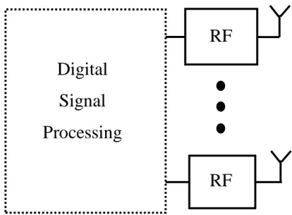
In MIMO systems, more than one antennas are equipped at both the transmitting side and receiving side. The conventional MIMO system mentioned in [20] is fully digital, which means all signal processing work are finished in baseband. Therefore, when the large scale antenna array is employed at any side in transmission, a large number of RF chains are required, which leads to the unaffordable energy consumption and cost in hardware. As a result, a fully analog architecture can be utilized to reduce the number of RF chains required. The phase shifter are employed to adjust signal to achieve an array gain, which process can be explored as analog beamforming. In Fig. 2.2 and Fig. 2.3, the signal process with fully digital architecture and fully analog architecture are shown respectively.

(25)

2.1. mmWaveBandCommunications 13

Linear

array

φ

Circular

array

Rectangular

array

φ

(26)

Digital

Signal

Processing

RF

Figure 2.2: Fully digital MIMO architecture.

Analog

Signal

Processing

RF

(27)

2.1. mmWaveBandCommunications 15

Rx

Tx

Wireless

Channel

Figure 2.4: The architecture of SU-MIMO system.

Rx

Tx

Wireless

Channel

Rx

(28)

As defined in [16], compared with single input single output (SISO) systems, which only have single antenna equipped at both the transmitter and the receivers, MIMO systems use multiple antennas at both sides. MIMO offers higher capacity and reliability. Also, in terms of the multiplexing, diversity and array gains, the MIMO channels have considerable advantages over SISO channels.

MIMO systems have two basic configurations, which can be divided into the single user MIMO (SU-MIMO) and multi-user MIMO (MU-MIMO) systems, which are shown in Fig. 2.4 and Fig. 2.5, respectively. Linear antenna array is considered in both systems. Single active UE is served or scheduled in a transmission time interval (TTI) in SU-MIMO systems, while the large scale antenna arrays are equipped at both transmitter and receiver. In this kind of system, the single UE transmission means that all time-frequency resource are allocated to one terminal, which means the diversity in spatial domain is ignored. Compared with SU-MIMO, in MU-MIMO systems, the same time-frequency resource are reused by multiple UEs. The multi-UE diversity is considered in spatial domain, which brings large gains compared with SU-MIMO, especially in the cases that channels are spatially correlated.

Except from the advantage of the spatial diversity usage, compared with SU-MIMO sys-tems, single antenna can be employed by each UE in MU-MIMO systems. In this case, the expensive equipment is just needed at the BS, which results in a large cost reduction.

In the comparison between SU-MIMO and MU-MIMO systems, last but not least, a rich scattering is seldom required in MU-MIMO systems because they are relatively less sensitive to the propagation environment. This feature may be beneficial to reduce the complexity of channel estimation in MU-MIMO systems.

(29)

2.2. AoA Estimation inMIMO System 17

2.2 AoA Estimation in MIMO System

2.2.1 Receiving Signal Model with Uniform Linear Array

Plane Wave 𝜃 dsin𝜃 d 2 1 3 N

Figure 2.6: Plane wave arrives at ULA with AoAθ.

The uniform linear array (ULA) with N elements is employed to receive signals. As shown in Fig. 2.6, the distance between adjacent antennas isd, the plane wave is assumed to hit the antenna array with an angle θ. The angle θ is the AoA of the receiving signal plane wave, which is measured clockwise from the vertical line of the antenna array. In this section, the model of receiving signal vector on a ULA for AoA estimation is detailed.

In Fig. 2.6, a time delay (i−1)τcan be found for the signal received at theith(i=1,· · · ,N) element of the array antenna compared with the first element. Therefore, the signal at the ith

(30)

element in the time domain is expressed as

xi(t)= x(t−(i−1)τ)= ej2πf t·e−j2πf(i−1)τ, (2.4)

where jrepresents the imaginary unit of a complex number, f is the carrier frequency,xis the transmitted signal. The time delay between adjacent antennasτis

τ= dsinθ

c =

dsinθ

fλ0

. (2.5)

λ0is the corresponding wavelength for the carrier frequency f. Substitute τin Eq. (2.4) with Eq. (2.5) xi(t) = e j2πf t_· e−j2πf(i−1)dsin θ fλ₀ = ej2πf t_·_e−j2π(i−1)dsinλ₀θ = ej2πf t ·e−j(i−1)ψ . (2.6) ψ= 2πdsinθ

λ0 is only decided by the AoA of signal on a specific antenna array with a fixed carrier frequency, it is seen as a new expression of AoA in the following equations for simplification. Considering the Additive White Gaussian Noise (AWGN) in the channel for transmission, the receiving signal vector with sizeN×1 at the antenna array can be written as

y(t)=                                  1 e−jψ e−j2ψ ... e−j(N−1)ψ                                  x(t)+                                  n1(t) n2(t) n3(t) ... nN(t)                                  . (2.7)

WhenMsignals are received at the antenna array simultaneously with different AoAψ

1, ψ1,· · · , ψM,

the receiving signal vector model at ULA is

y(t) = M P m=1 α(ψm)xm+n(t) = Ax(t)+n(t) , (2.8)

(31)

where α(ψm) =

h

1,e−jψm,_{· · ·} ,_e−j(N−1)ψmiT _{is defined as steering vector for the} _mth _signal,

[·]T represents the transpose of a matrix or vector, A=α

(ψ1), α(ψ2),· · · , α(ψM). x(t) =

h

x1,x2,· · · ,xMiT represents all the transmitting signals, andn(t) = [n1(t),n2(t),· · · ,nN(t)] T

is the noise vector. y(t) is the temporal sample of array receiving signal for the time instant t (snapshot t). A large number of temporal samples taken in the period with unchanged Aare helpful for improving the AoA estimation accuracy.

2.2.2 Conventional AoA Estimation Methods

The antenna array based AoA estimation methods can be divided into the subspace methods and non-subspace methods [22]. it is mentioned that compared with subspace methods, some non-subspace methods, such as the maximum likelihood methood, have computational inten-sive searching step and have poor performance in terms of estimation resolution. The MUSIC algorithm and ESPRIT algorithm belong to subspace methods, both of them are popular and widely utilized. In this section, the principles and procedures of MUSIC and ESPRIT algo-rithms are detailed, while their estimation resolution are compared in the cases with different numbers of signal snapshots, and in manifold SNR environments.

The main idea of MUSIC algorithm is to separate the signal space and noise space accord-ing to the orthogonality, the separation is achieved by the eigendecomposition step operated on the average array covariance matrix of the receiving signal. As the algorithm for comparison with the novel algorithm in the thesis, the MUSIC algorithm is detailed as follows.

In the MUSIC AoA estimation algorithm, the number of antennas in the receiving array should be ensured to be larger than the number of signals, i.e. N > M. The whole algorithm can be divided into four steps:

• Construct the average array covariance matrix based on the receiving signal vector; According to the receiving signal vector defined in Eq. (2.8), the matrix can be expressed as ¯ Ryy= E h yyHi= AEhx1x1H i AH+σ2nI, (2.9)

(32)

noise variance,E[·] is the expectation operator based on multiple signal snapshots.

• Obtain the eigenvalues and eigenvectors of correlation matrix by eigendecomposition, resort eigenvalues and eigenvectors;

After the operation of eigendecomposition,Neigenvalues and their corresponding eigen-vectors can be obtained. Sort the eigenvalues from the largest value to the smallest value, at the same time change the order of eigenvectors. The reordered matrix for eigenvectors is [v1,v2,· · · ,vM,vM+1,· · · ,vN].

• FormN−Meigenvectors with the smallest eigenvalues into the matrix of noise subspace; The matrix of noise subspace isVn =[vM+1,· · · ,vN], it satisfies

[vM+1,· · · ,vN]⊥α(ψ1), α(ψ2),· · · , α(ψM)

⇒ _αH₍_ψ

m)VnVnHα(ψm)= 0, (m=1,· · · ,M)

, (2.10)

Eq. (2.10) means the signal space, which is represented by the steering vectors of signal components are orthogonal to the noise subspace eigenvectors.

• Scan the range of angle to create spatial spectrum, the angles located at peaks of spatial spectrum are the estimated AoA ˆθm(m=1,· · · ,M).

With the matrix of noise subspace, the MUSIC spatial spectrum can be generated by the steering vectors scanning in the range of angle as below

P(ψ)= 1 αH₍ψ₎_V nVHnα(ψ) ψ= 2πsinθ λ0 , θ ∈[−90 ◦_, 90◦] , (2.11)

By locating the peaks of the spatial spectrum, the AoA of the signals can be estimated. Fig. 2.7 gives an example of MUSIC spatial spectrums. Comparing different curves, the influence of SNR and snapshots can be found. 8 antennas are employed on the receiving array, and the AoA for two signals are estimated at the same time, for which the AoA are fixed as -30 degrees and 30 degrees. It shows that the spikes are becoming more definite with the increase of SNR, while the performance rises sharply with more available snapshots.

(33)

Figure 2.7: The MUSIC spatial spectrums for two signals AoA estimation with different SNR and numbers of snapshots.

The ESPRIT algorithm decomposes an antenna array with N sensors into two identical subarrays,Neelements are equipped at each subarray, while the distance between two subarrays

is known. It is the objective of this algorithm that estimating AoA by calculating the operator

ϕe for the rotation from signal on one subarray to that on the other one.

Suppose that Ne = N−1 for each subarray, and the distance between two subarrays is d.

Matrixes of steering vectors for both subarrays are part ofAfor the whole antenna array, which is A1=                          1 e−jψ1 ... e−jNeψ1 · · · · · · · · · · · · 1 e−jψM ... e−jNeψM                          , A2 =                          e−jψ1 e−j2ψ1 ... e−j(Ne+1)ψ1 · · · · · · · · · · · · e−jψM e−j2ψM ... e−j(Ne+1)ψM                          . (2.12)

(34)

of signal. The expression offT is

fT =                          e−jψ1 ₀ _{· · ·} ₀ 0 e−jψ2 _{· · ·} ₀ ... ... ... ... 0 0 · · · e−jψM                          , (2.13)

When the subarray distance and the carrier frequency of each signal are known, the AoA of each signal can be calculated fromfT. However, the matrix of steering vectors of subarrays

cannot be recovered from receiving signals directly, hence,fT cannot be obtained. In the

ES-PRIT algorithm, based on the fact that the steering vectors in matrixAspan the same subspace asVs = [v1,· · · ,vM], therefore, the signal subspaceVsis utilized to generate the matrixes of

eigenvectors forA1andA2, which are represented byV1andV2, respectively. There exists an invertible matrixTto achieve the transform fromA1,A2 toV1andV2, which brings

V1 =A1T

V2 =A2T=A1fTT

, (2.14)

the relationship betweenV1andV2is

V1 =V2T−1fT−1T, (2.15)

[·]−1 represents the inverse of a matrix. RecordF−1

T = T

−1_f−1

T T, therefore, V1 = V2F−T1, i.e.

V2 =V1FT. fT is a diagonal matrix of the eigenvalues ofFT. WithFT,fT can be obtained, and

the AoA of signals can be calculated.

On the basis of the aforementioned principles, the ESPRIT algorithm can be achieved by the following steps:

• Construct the input correlation matrixR¯yy based on the receiving signal vector, find its

signal subspaceVsby eigendecomposition;

• Extract signal subspaces of subarraysV1andV2fromVs;

(35)

2.2. AoA Estimation inMIMO System 23 the estimatedFT isFˆT = VH 1V1 −1 VH 1V2;

• The diagonal matrix for the eigenvalues ofFˆT is the estimated ˆfT, the estimated AoA of

signals in degrees are obtained by ˆθm=−180_π sin

−1arg(e−jψm)λ0 2πd

, (m=1,· · · ,M).

Figure 2.8: The comparison of MUSIC algorithm and ESPRIT algorithm with different SNR and increasing numbers of snapshots.

In Fig. 2.8, The root mean square error (RMSE), which is defined as Eq. (2.16), is com-pared between MUSIC algorithm and ESPRIT algorithm in the environment with low and high SNR (−5dBand 25dB) SNR and with different numbers of snapshots. Nep times of

ex-periments are done to calculate each point in the figure to prevent the influence of abnormal results. The number of antennas in the whole array is 8, while 7 antennas are allocated to each subarray. Similar performance can be found for both of the algorithms with any SNR or number of snapshots, while the low RMSE, which means the high estimation resolution can be provided by two algorithms in high SNR environments with only several snapshots. However, with low SNR, more snapshots are required for high estimation resolution. Therefore, the high

(36)

resolution AoA estimation is still an open issue in low SNR environment with few snapshots.

RMS E=         1 MNep Nep X n=1 M X m=1 θm− _ θm !2        1/2 , (2.16)

2.2.3 Applications of Neural Network in AoA Estimation

Many research works are focusing on the neural network based high resolution AoA estimation methods, in order to achieve accurate AoA estimation for different cases. The convolutional neural network (CNN), radial basis function neural network (RBFNN) and the multi-layer perceptron (MLP) based neural networks are three kinds of popular neural network models which have been studied for a long time. Many papers can be found about their applications in AoA estimation.

The structure of the CNN model for beam based AoA estimation designed in [23] is shown in Fig. 2.9. It can be found that the CNN model is consisted of convolutional layers, sub-sampling layers and fully-connected layers. The convolutional layers are used to extract the high-level features such as edges, from the input nodes. In this model, each convolution plane is connected to one or more subsampling planes. In fact, the subsampling layers are always set after convolutional layers, which are designed to downsample the output of convolutional layers. The fully-connected layer is utilized as the output layer of this model. The CNN model designed in [23] is mentioned to be capable to select the suitable radiation beams without the knowledge of the source signals number, while the signals are received from different direc-tions. The input covariance matrix defined in Eq. (2.9) is utilized to generate input matrixXin,

while the output Yout are the beams indices selected for each signal. In this AoA algorithm,

although ranges of the selected beams can always cover the directions of signals, the estimation resolution is not high for it is limited by the coverage of beams in angle domain.

The RBFNN models are utilized with relatively fixed structure, so the number of neurons in hidden layer is very important for the performance of model [24]. The model is named as this because the radial basis function is used in the hidden layer of model. It is said that the RBFNN with enough hidden neurons can approach to functions with any resolution. To

(37)

2.2. AoA Estimation inMIMO System 25 Convolutional Layer 2 Subsampling Layer 2 Subsampling Layer 1 In p u t N od es X in Ou tp u t N od es Y ou t Convolutional Layer 1 Output Layer Last Convolutional Layer Output Neuron

Convolution Plane Subsampling Plane

Figure 2.9: The structure of a CNN model.

be mentioned that the input nodes shown in Fig. 2.10 for this model should be the vectored covariance matrix, while the output nodes are the AoA of signals. The mapping function of RBFNN in hidden layer is given in Eq. (2.17)

Yout =F(Xin)= L

X

l=1

wlφ(kbl−Xink), (2.17)

whereφ(x) is the radial basis function of x, andk·krepresents the 2-norm operation. Lis the number of neurons in the hidden layer,wlrepresents the weight of hidden neurons, while thebl

is the center vector for the radial basis function, which is usually determined through K-means clustering. The radial basis function φ(x) is usually assumed to be un-normalized Gaussian function, which is

φ(x)= e −x2

2σ2, (2.18)

(38)

structure of RBFNN, the AoA estimation error of this model can hardly be low enough.

ԡ∙ԡ

∅ሺ∙ሻ

Ou

tp

u

t N

od

es

Y

ou t

In

p

u

t N

od

es

X

in

Hidden Layer

𝝎

_𝐿

𝝎

1

𝝎

_𝑙

−𝒃

₁

−𝒃

_𝑙

−𝒃

𝐿

Figure 2.10: The block diagram representation of the RBFNN.

The MLP neural network is a kind of multi-layer and nonlinear neural network [25]. Com-monly a MLP neural network is consisted of multiple layers, which include an input layer, hidden layers and an output layer. Nonlinear activation functions can be selected for each fully-connected layer (FCL) neuron, after the activation layer (AL) these neurons are con-nected with the neurons in the next layer. Multiple hyperparameters are needed for the MLP model structure design, including the number of hidden layers, the number of neurons for each layer, the activation functions selection, and so on. These predefined hyperparameters make the MLP neural network design become flexible, in order to satisfy any kinds of input-output mapping requirements. The structure of MLP neural network model is shown in Fig. 2.11. Many MLP neural network based AoA estimation algorithms have been proposed to provide high resolution results, while the large potential still can be found for both high resolution and robust estimation by MLP neural network model due to its high flexibility.

(39)

2.3. FDD/TDD Communications 27

Input

Layer

In

p

u

t N

od

es

X

in

Ou

tp

u

t N

od

es

Y

ou t

Output Layer

FCL AL

A

C

T

I

V

A

T

I

O

N

Hidden Layer 1

FCL AL

A

C

T

I

V

A

T

I

O

N

Figure 2.11: The structure of MLP neural network.

2.3 FDD

/

TDD Communications

2.3.1 Frame Structures for FDD

/

TDD

#0 #1 #2 #3 #18 #19

One radio frame, Tf = 307200Ts = 10 ms

One slot, Tslot = 15360Ts = 0.5 ms

One subframe

Figure 2.12: Frame structure type 1.

In this section, the frame structures for TDD systems and FDD systems are compared to prove the requirement of separate beamforming designs for different systems. The frame structure type 1 is defined for FDD scenario in 3GPP TS 36.211 [21], which is shown Fig. 2.12. For both

(40)

full duplex and half duplex FDD, 10 subframes, 20 slots, or up to 60 subslots are available for both uplink and downlink transmissions in each 10msinterval. Compared with the half-duplex FDD systems, the full-duplex FDD has fewer restrictions, it can transmit and receive signal at the same time.

One slot,

Tslot=15360Ts

GP UpPT_S DwPTS

One radio frame, Tf = 307200Ts = 10 ms

One half-frame, 153600Ts = 5 ms 30720Ts One subframe, 30720Ts GP UpPT_S DwPTS

Subframe #2 Subframe #3 Subframe #4

Subframe #0 Subframe #5 Subframe #7 Subframe #8 Subframe #9

Figure 2.13: Frame structure type 2 (for 5 ms switch-point periodicity).

Frame structure type 2 is only applicable to TDD systems. As shown in Fig. 2.13, the frame structure is similar to that of FDD systems, for each 10msradio frame, 10 subframes are equally divided, each of which can be further split into two slots. The signals cannot be transmitted and received simultaneously, therefore, it is mentioned that this type of frame structure can support two kinds of switch-point periodicities for the conversion of uplink and downlink signals, one subframe is required for the downlink pilot time slot (DwPTS), uplink pilot time slot (UpPTS) and guard period (GP). The smallest downlink-to-uplink switch-point periodicity is 5ms, which is much higher than the coherence time of mmWave channel even if the UEs are moving in a low speed. Here the coherence time is the period over which the channel impulse response (channel matrix) is considered to be unchanged. When carrier frequency f = 38GHz, UE moving speedv= 5m/s, the coherence timeTcois

Tco =

0.423

v f/c ≈0.63ms< 5ms, (2.19)

herec= 3×108is the speed of light. Therefore, the uplink signal is not always available in each coherence time, which means the beams can hardly be selected for downlink transmission adaptively. Based on the difference of frame structures for TDD and FDD systems, it can be

(41)

2.4. Beamforming inMIMO System 29

concluded that the most significant difference between two systems is the availability of uplink signal during the downlink transmission. Due to this difference, the beamforming algorithms should be designed separately to adapt to different systems.

2.4 Beamforming in MIMO System

2.4.1 Types of Beamforming

With the development of massive MIMO system, the beamforming technique is explored based on the large scale antenna array for its advantage of large power gain. In MU-MIMO system, the beamforming design can not only improve the link quality, but also reduce the influence of interference [26].

In many beamforming methods, the transmitting beamformers are designed with the as-sumption of available full CSI. However, in practise, the transmitters with larger scale antenna arrays can only obtain partial CSI, such as the AoD of paths, based on the feedback in TDD systems communications or the channel reciprocity in FDD systems communications [27]. The codebook based beamforming and angle based beamforming are two kinds of partial CSI beamforming methods which are widely explored.

2.4.2 Codebook based Beamforming

The codebook based beamforming works to improve transmitting power and reduce interfer-ence by the perfect selection of codewords, which are generated based on the codewords from a codebook. Here the codebook is defined as a matrix consisted of vectors for precoding (beams generation). The beam training step is always required to find out the best transmit-ting/receiving beams for UEs, which should be suitable to their CSI. In the beam training step for regular codebook based beamforming, the beams using all codewords as precoders are transmitted, after which the indices of codewords brings large power gain and small interfer-ence are feedbacked for the beams generation in the data transmission. This kind of training

(42)

process is called exhaustive search training, this training method is conceptually straightfor-ward. However, because of the large number of candidate codewords in the codebooks for mmWave communication, the overall search time is prohibitive, and a large amount of resource is wasted as the training and feedback overhead.

To reduce the overhead for the beam training step while keeping the advantage of perfect codeword selection, the hierarchical codebook is designed in [28], which is utilizing codewords from several layered codebooks for training, the beams generated by codewords from different layered codebooks have diverse beamwidth and power gain. The principle of the hierarchical codebook is to train beams generated by codewords from the lowest layer to the highest layer. Not all of the codewords are needed to be trained in each layered codeword because the training range on the angle domain is narrowed by the selected codeword range in the last layer. Two basic criteria should be satisfied to design the hierarchical codebook, which are:

1. The beam coverage union generated by all the codewords in each codebook should be able to cover the whole angle domain;

2. The coverage of each beam generated by a codeword from a non highest-layer codebook should be covered by the coverage union of a couple of codewords in the next layer.

The hierarchical codebook is designed for the codeword selection at both the transmitting side and receiving side, for the two sides the designing principles are totally the same. For the

cth₍_c= ₁, . . . ,_C₋_{1) layer codebook, the range of beams generated by}_C

wadjacent codewords

in the (c+1)th layer should cover the beamwidth of a codeword in thecthlayer. The highest-layer codebook is firstly designed withN codewords, which number is equal to the number of antennas. Each codeword can be expressed as

w(C,in)=α(N,−1+(2in−1)/N), (in= 1, . . . ,N) , (2.20)

α(N,sinθ)= √1 N

h

1,ejπsinθ, . . . ,ejπ(N−1) sinθiT. (2.21) The number of layersC = log_C

w(N). For the codewords in the layerc = logCw(N)−k, where

(43)

1. The elements inw(c,1) can be uniformly divided intoL=Cf loor(

k+1 2 )

w groups, each group

is wl(c,1)= [w(c,1)](l−1)N

L+1:lNL, (l=1, . . . ,L) ;

2. Ifkis odd, setNL = L/2; else,NL= L. wl(c,1) is set as

wl =            e−jlN_N−LπαN L,−1+ L(2l−1) N , l= 1, . . . ,NL 0N L×1, l= NL+1, . . . ,L ; (2.22) 3. w(c,in)=w(c,1)◦ √NαN,2(_Cin−1) wc , (in= 2,3, . . . ,Cwc) . 4. Normalizew(c,in).

Where◦represents entry-wise product. An example of the hierarchical codebook is shown on Fig. 2.14. A multi-sectional search beamforming algorithm is proposed in [28] utilizing the hierarchical codebook. When the hierarchical codebooks utilized at the transmitting side and the receiving side are totally the same, it requires 2log_C

wN bits for the training, and other

2logCwN bits for the feedback for each receiver in order to select suitable codewords for both

precoding and receiving. For the application of hierarchical codebook in the MU-MIMO sys-tem, a large scale antenna array serves multiple single-antenna UEs in the downlink, therefore, log_C

wN bits are needed for downlink training and uplink feedback, separately, which means

2logCwN are used for the perfect precoding codeword selection of a UE. It can be found that

the large number of antennas at the transmitting side brings large overhead for codewords se-lection.

The SWR oriented beamforming designed based on the hierarchical codebook further re-duces the overhead for codebook based beamforming while the SR is partly sacrificed [29][67]. This algorithm also searches the suitable codeword for a UE from the lowest layer to the high-est layer. However, the SWR is considered in the algorithm design, which is the parameter reflects both the influence of overhead and SR. In the training process, when the SWR is esti-mated to reduce with the further training, the training step stops and the best codeword in the current layer codebook is selected.

(44)

-1

w

(2,1)

w

(2,Cw)

w

_(C(2,Cw w-1)+1)

w

(1, Cw)

w

(2,Cw2)

w

(1,1)

w

(C,N)

w

(C,1)

1

st

_layer

2

nd

_layer

C

th

_layer

1 Angle domain (

sinθ

)

Figure 2.14: Hierarchical codebook for analog beamforming.

2.4.3 Angle based Beamforming

Angle based beamforming makes full use of the AoD of dominant paths in the transmission channel. As a partial CSI based beamforming, getting the angle information of paths is much easier than obtaining the full CSI information. In TDD systems, the uplink pilot signal can be utilized to estimate the downlink CSI directly due to the channel reciprocity; While in FDD systems, for the cases that the carrier frequencies of uplink and downlink channels are not far away from each other, the AoA estimated for the uplink paths can be viewed as the AoD for the corresponding downlink paths, when the time elapse between uplink and downlink signals can be neglected [9][30].

With the AoD information of dominant paths, the angle based beamforming can be de-signed to increase the power gain in the required directions, while reduce the power gain in the interference directions. The beamforming design can be applied on both analog and digital parts. The angle based analog beamforming vector for themthUE with AoDθmis

wm_A(N,sinθm)= 1 √ N h 1,ejπsinθm, . . . ,_ejπ(N−1) sinθmiT. _(2.23)

(45)

(a)

(b)

Figure 2.15: The comparisons among hybrid beamforming withN = 8 of (a) AoD of interfer-ence UE is−15◦(b) AoD of interference UE is−38◦.

(46)

Compared with the analog beamforming design, the digital beamforming considers not only the AoD of the aim UE, but also that of other UEs. Therefore, the estimated AoD matrix

H=[α(N,sinθ1), α(N,sinθ2),· · · , α(N,sinθm)] H

should be utilized for digital beamforming design. The zero forcing (ZF) digital algorithm is widely used in digital precoder design, which is chosen as an example [8]

WZF =HH

HHH−1. (2.24)

However, in the applications with large scale antenna arrays, the size of matrixHis too large to apply the digital beamforming in a limited time. The hybrid beamforming is designed to face this challenge, it utilizes both analog and digital beamforming at the same time. This means the ZF algorithm can work on the dimension-reduced AoD matrix in this example, which is

WAZF =HHA HAHHA −1 , (2.25) HA =HWA, (2.26) whereWA = h w1 A,w2A,· · · ,w M A i

is the matrix of analog beamforming vectors forMUEs. It is the fact that compared with analog beamforming, the digital beamforming is designed based on all UEs AoD vector, i.e. for a specific aim UE with fixed AoD, the difference on the AoD of interference UEs brings different digital beamforming design, while the analog beamforming for this UE is always the same. Fig. 2.15 compares the hybrid beamforming design for an aim UE with fixed AoD, while the interference UE has different AoD. The totally different beam patterns (power gain and beamwidth) prove our conclusion. We can also find that the hybrid beamforming can work to reduce interference to other UEs with any dominant path AoD with flexibility. However, this may reduce the power of signal to the aimed UE.

2.5 Chapter Summary

This chapter starts from the introduction to the mmWave channel and the MIMO system in mmWave communicatons. Except from the configurations of antenna arrays and two kinds of signal preprocessing methods with MIMO, the SU-MIMO and MU-MIMO systems are

(47)

2.5. ChapterSummary 35

detailed as well. After that, the antenna array based AoA estimation is review in the second section. The receiving signal model is introduced at first, based on that the procedures of AoA estimation by MUSIC and ESPRIT algorithms are shown step by step, the numerical results for the performance of MUSIC and ESPRIT algorithms with diverse SNR and snapshots are given, which show the challenge in conventional AoA estimation explicitly. Then the neural networks with different structures and used to be mentioned in AoA estimation methods design are discussed to compare their characteristics. In Section 2.3 and 2.4, the frame structures of TDD and FDD systems are compared to prove the necessity of separated beamforming designs in different systems. Then in the last section, some low overhead partial CSI beamforming methods including the codebook and angle based beamforming, are introduced and compared.

Exploitation of Robust AoA Estimation and Low Overhead Beamforming in mmWave MIMO System

Scholarship@Western

Scholarship@Western

Exploitation of Robust AoA Estimation and Low Overhead

Exploitation of Robust AoA Estimation and Low Overhead

Beamforming in mmWave MIMO System

Beamforming in mmWave MIMO System

Abstract

Lay Summary

Acknowledgements

Contents

List of Figures

List of Tables

List of Abbreviations

Chapter 1

Introduction

1.1

Overview of Communications with Large Scale Antenna

Array

Biomedical

Imaging

Radar

Remote

Sensing

Navigation

Vehicular

Communi

-cations

1.2

Thesis Motivations

1.3

Research Objectives

1.4

Technical Contributions of the Thesis

1.5

Thesis Outline

Chapter 2

AoA Estimtion and Beamforming Design

in mmWave MIMO System

2.1

mmWave Band Communications

2.1.1

Characteristics of mmWave Band Communications

2.1.2

MIMO in mmWave Communications

Linear

array

φ

Circular

array

Rectangular

array

φ

Digital

Signal

Processing

RF

RF

Analog

Signal

Processing

RF

RF

Rx

Tx

Wireless

Channel

Rx

Tx

Wireless

Channel

Rx

Rx

2.2

AoA Estimation in MIMO System

2.2.1

Receiving Signal Model with Uniform Linear Array

2.2.2

Conventional AoA Estimation Methods

2.2.3