System reliability when components can be swapped
upon failure
NAJEM, AESHA,MOHAMMAD,M
How to cite:
NAJEM, AESHA,MOHAMMAD,M (2019) System reliability when components can be swapped upon failure, Durham theses, Durham University. Available at Durham E-Theses Online:
http://etheses.dur.ac.uk/13110/
Use policy
The full-text may be used and/or reproduced, and given to third parties in any format or medium, without prior permission or charge, for personal research or study, educational, or not-for-prot purposes provided that:
• a full bibliographic reference is made to the original source
• alinkis made to the metadata record in Durham E-Theses
• the full-text is not changed in any way
The full-text must not be sold in any format or medium without the formal permission of the copyright holders. Please consult thefull Durham E-Theses policyfor further details.
components can be swapped upon
failure
Aesha M. Najem
A Thesis presented for the degree of
Doctor of Philosophy
Department of Mathematical Sciences
University of Durham
England
2019
swapped upon failure
Aesha M. Najem
Submitted for the degree of Doctor of Philosophy
April 2019
Abstract
Resilience of systems to failures during functioning is of great practical impor-tance. One of the strategies that might be considered to enhance reliability and resilience of a system is swapping components when a component fails, thus replac-ing it by another component from the system that is still functionreplac-ing. This thesis studies this scenario, particularly with the use of the survival signature concept to quantify system reliability, where it is assumed that such a swap of components re-quires these components to be of the same type. We examine the effect of swapping components on a reliability importance measure for the specific components, and we also consider the joint reliability importance of two components. Such swapping of components may be an attractive means toward more resilient systems and could be an alternative to adding more components to achieve redundancy of repair and replacement activities.
Swapping components, if possible, is likely to incur some costs, for example for the actual swap or to prepare components to be able to take over functionality of an-other component. In this thesis we also consider the cost effectiveness of component swapping over a fixed period of time. It is assumed that a system needs to function for a given period of time, where failure to achieve this incurs a penalty cost. The expected costs when the different swap scenarios are applicable are compared with the option not to enable swaps. We also study the cost effectiveness of component swapping over an unlimited time horizon from the perspective of renewal theory. We assume that the system is entirely renewed upon failure, at a known cost, and
we compare different swapping scenarios. The effect of components swapping on preventive replacement actions is also considered.
In addition, we extend the approach of component swapping and the cost effec-tiveness analysis of component swapping to phased mission system. We consider two scenarios of swapping possibilities, namely, assuming that the possibilities of component swapping can occur at any time during the mission or only at transition of phases.
The work in this thesis is based on research carried out at the Department of Mathe-matical Sciences, Durham University, UK. No part of this thesis has been submitted elsewhere for any other degree or qualification and it is all my own work unless referenced to the contrary in the text.
Copyright c 2019 Aesha M. Najem.
“The copyright of this thesis rests with the author. No quotations from it should be published without the author’s prior written consent and information derived from it should be acknowledged”.
All praise due to the Almighty Allah, without His great help, this work could not have been done.
I am speechless and cannot express my deep thanks and gratitude to my su-pervisor Professor Frank Coolen. He was very supportive and kind. I will never forget how much time he gave me. Without his patience, insightful comments and guidance, I could not have overcome many obstacles I faced and my thesis could not have been completed. So, thank you so much for everything you have done for me during your invaluable supervision period on my research.
My parents were my source of strength, thank you my beloved mother Khadija and my great father Muhammad. Without you both and your countless support, I could not reach this happy ending today.
My dearest gratitude to my family, my dear husband Amin, who was very sup-portive for many years, not only during my PhD study, but in all my life aspects. I really cannot find the words to thank him. My beloved children: Ahmed, Ibtihal, Omar and Ibrahim, who are my life, always empowered me in my hard times. Thank you all for your endless support, patience and understanding. I can tell you now, your mum finally has finished.
My thanks also to my sponsor, the Saudi Electronic University for facilitating my scholarship and continually supporting me.
My thanks and gratitude are extended to Durham University Mathematics De-partment for the help and support they offered me. I cannot forget to thank my classmates at the Department for their kindness and great time we had together.
Abstract iii Declaration v Acknowledgements vi 1 Introduction 2 1.1 Resilience . . . 5 1.2 System reliability . . . 5 1.2.1 Structure function . . . 6 1.2.2 Reliability measurement . . . 9 1.3 Reliability importance . . . 11
1.4 The survival signature . . . 14
1.5 Research aim and objectives . . . 18
1.6 Outline of the thesis . . . 19
2 System reliability and component importance when components can be swapped upon failure 21 2.1 Introduction . . . 21
2.2 Swapping components . . . 22
2.2.1 Alternative approach . . . 27
2.3 Component reliability importance . . . 37
2.4 Joint reliability importance (JRI) . . . 47
2.5 Concluding remarks . . . 50
3 Cost effective component swapping to increase system reliability 54
3.1 Introduction . . . 54
3.2 Penalty costs for system failure with component swapping . . . 55
3.2.1 Time independent penalty costs . . . 55
3.2.2 Time dependent penalty costs . . . 56
3.3 Optimal swapping based on renewal theory . . . 60
3.3.1 Preventive Replacement . . . 62
3.4 Concluding remarks . . . 66
4 Phased mission systems with components swapping 68 4.1 Introduction . . . 68
4.2 Phased mission systems . . . 71
4.3 Swapping components upon failure . . . 72
4.3.1 PMS with single type of components . . . 72
4.3.2 PMS with multiple types of components . . . 78
4.4 Swapping components according to structure importance . . . 85
4.5 Cost analysis of PMS with component swapping . . . 93
4.5.1 Time independent penalty costs . . . 94
4.5.2 Time dependent penalty costs . . . 95
4.6 Concluding remarks . . . 105
5 Concluding Remarks 107
Introduction
With the need for highly reliable systems, there are many possibilities to make a basic system more reliable or more resilient to possible faults. It may be possible to add component redundancy or make individual components more reliable. In addition, one may be able to repair failed components or replace them with new ones. In this thesis, we consider a quite straightforward way in which some systems may become more reliable and resilient to component failure, namely, the possibility to replace a failed component by another component in the system that has not yet failed, in effect swapping components. This is logically restricted to components which are of the same type, hence it is likely that only some swapping opportunities exist in a system. It seems that the increase in system reliability through such component swapping has not received much attention in the literature, yet in some scenarios it can be an attractive opportunity to prevent a system from failing. In practice, this could enable preparation of substantial repair activities, or it may be deemed to leave the system reliable enough to complete its mission.
Scenarios where swapping of components may be an option can include the fol-lowing examples. Aerospace systems with multiple computers on board, where some computers tasked with minor functions can be prepared to take over crucial functions in case another computer fails. Lighting systems, where multiple locations must be provided with light under contract but where partial lighting at any location may be sufficient to meet the contractual requirements. Transport systems, where parts of one mode of transport can be used to keep another one running. Organizations,
where employees can be trained to take over some functioning of others in case of unexpected absence.
It should be emphasized that swapping a component, upon failure, with another component from the system, differs from the well-studied scenarios of using cold or warm standby components or adding components in parallel to achieve increased reliability [25, 33, 61, 71]. When we replace a failed component with a functioning component that was already in the system, the subsystem, in which the later compo-nent was originally placed, becomes less reliable. One can also compare the kind of component swapping studied in this thesis to a minimal repair [60], in that the fail-ure time distribution of the component does not change, but this is combined with a change in the overall structure of the system due to the functioning component being removed elsewhere.
In this thesis we consider the effect of defined component swap possibilities on the total system reliability. We also consider the importance of individual components, which can be strongly affected by opportunities to swap them and the joint reliability importance (JRI) of two components. The survival signature concept is used to derive the corresponding system reliability [18].
A system is usually designed and installed for completing a specific function. If a system fails, it can cause losses such as loss of lives, damage to health, release of hazardous materials, or economic losses including repair or replacement of any damaged structures. These losses incur costs. It would be attractive if the cost that is associated with system failure could be reduced by increasing system reliability through component swapping. The operation of swapping components is likely to incur some costs, for example for the actual swap or to prepare components to be able to take over functionality of another component. This thesis also consider the cost effectiveness of component swapping to increase system reliability. The cost aspects is studied under the assumption that a system would need to function for a given period of time, where failure to achieve this incurs a penalty cost. We compare different swap scenarios with the option not to enable swaps, focusing on minimum expected costs over the given period. We also consider the cost effectiveness of component swapping from the perspective of renewal theory, so effectively over an
unlimited time horizon. We assume that the system is entirely renewed upon fail-ure, at a known cost, and we compare different swapping scenarios. The effect of components swapping on preventive replacement actions is also considered [64].
A phased mission system (PMS) is one that performs several different tasks or functions in sequence. In order to accomplish the mission successfully, the system in every phase has to be completed without failure. Therefore, it is often difficult for a PMS to work with high reliability. Generally, there are mainly two approaches that can be used to improve the reliability of the PMS. The first way is increasing the component reliability (reliability allocation), and the other way is using redundant components in parallel (redundancy allocation) e.g. [3, 23, 43, 50]. As an alternative to these approaches, in this thesis we introduce the approach of component swapping to enhance the reliability of phased mission system and to make it more resilient to component failure. This approach is attractive since the reliability and the number of the components do not need to be increased to improve the system reliability as the other approaches. We consider two strategies of components swapping to improve the reliability of PMS, namely, swapping components upon failure and swapping components according to structure importance. The effect of both strategies on the reliability of the PMS is studied under two scenarios of swapping possibilities. First, it is assumed that the swap between components can be done at any time during the mission. Second, it is assumed that the swap between components can be done only at transition of phases. In this thesis we also study the effectiveness of the cost of component swapping in reducing the expected costs of the failure of the PMS. The expected costs when the two different scenarios of swapping possibilities are applicable are compared with the option not to enable swaps, focusing on minimum expected costs over the given period.
This introductory chapter is organized as follows. Section 1.1 introduces the concept of resilience. Section 1.2 briefly reviews the concepts related to system reli-ability and its measurement. Section 1.3 provides a brief introduction to relireli-ability importance. Section 1.4 introduces the concept of survival signature. Section 1.5 illustrates the aim and objectives of this research. A detailed outline of this thesis is given in Section 1.6, with details of related publications.
1.1
Resilience
The concept of resilience originated in the field of ecology. It is defined in this field as the speed with which an ecosystem returns to the equilibrium state after a perturbation [24]. After it emerged in the field of ecology, this concept is gradually developed into different research fields. Despite an increase in the usage of the term resilience, there is no universal agreement on its definition. It is defined variously in different research fields such as social [1], organizational [30] and economical [56] fields. In each research field the term has taken more specific meaning depending on the field that it is introduced in. Although the concept of resilience has been around for a long time, this concept is relatively new in the field of systems engineering [39]. Various definitions of the term resilience in the field of systems engineering have been reviewed by [36]. In this thesis, resilience is defined to be the ability of systems to recover quickly from failures.
In engineering systems redundancy is embedded in system design in order to make the system resilient to possible faults. This strategy causes increase in the cost of the system and does not always yield competitive results [69]. As an alternative to this strategy, component swapping that is introduced in this thesis could be embedded in system design, precisely, systems could be designed to be resilient through allowing its components to be swapped. This would ensure that the system returns to function quickly. In a more resilient system, the design of the system would allow for component swaps to be beneficial in practice.
1.2
System reliability
In this thesis we assume that the term system is used to describe the collection of
components when connected to each other in some way to create the whole system. We might consider any electronic devices as an example of a system. In this section we briefly introduce the notation and concepts related to system reliability and its measurement. In Section 1.2.1, we present the theory of structure function and we briefly discuss related concepts. In Section 1.2.2, we discuss reliability measurement based on the structure function.
1.2.1
Structure function
The main characteristic of any systems in this thesis is that the functioning state of the whole system is dependent on the functioning states of its components. To quantify if the system is functioning or failed, it is assumed that the system and each component are binary, which means that they are only in one of two possible states: functioning or failed. We use the indicator 1 to denote the system or component functions, and 0 to denote that the system or component fails.
Definition 1.2.1 For a system with m components, the state vector is a vector
x= (x1, x2, ..., xm)∈ {0,1}m, wherexiis a binary variable indicating the functioning
state of the component i, for each i, so xi = 1 if the ith component functions and
xi = 0 if the ith component fails [42]. The labelling of the components is arbitrary
but must be fixed to define x.
It is assumed that the state of the system is completely determined by the states of its components. A mapping called the structure function determines whether or not the system is functioning when its components are in specific states.
Definition 1.2.2 Consider the space {0,1}m of all possible state vectors for an
m-component system [42]. The structure function φ : {0,1}m −→ {0,1} is a
mapping that associates those state vectors x for which the system functions with
the value 1 and those state vectors x for which the system does not function with
the value 0.
The quantification of the structure function φ is dependent on the structure of a
system. The structure of a system shows how its components are connected to each other. The connection between components represents how functioning of the components influences the functioning of the system. A system is called coherent, if its structural function is non-decreasing and each its component is relevant [42]. In this thesis we consider only coherent systems. The following examples demonstrate
C
A B
Figure 1.1: A series system with three components
B A
C
Figure 1.2: A parallel system with three components
Example 1.2.1 (Series systems)
In a series system the components are connected to each other in series [2]. All the components in a series system must function for the system to function. Figure 1.1 shows an example of a series system consisting of 3 components. The structure
function of a series system consisting ofm components is
φ(x) =
m
Y
i=1
xi (1.2.1)
Example 1.2.2 (Parallel systems) In a parallel system, the components are
con-nected to each other in parallel [2]. A parallel system functions, if at least one of its components functions. For the system to be failed, all of its components must be failed. Figure 1.2 shows an example of a parallel system consisting of 3 components.
The structure function of a parallel system consisting ofm components is
φ(x) = 1−
m
Y
i=1
(1−xi) (1.2.2)
Example 1.2.3 (Series-parallel and series systems) Series-parallel and
parallel-series systems consist of only combinations of subsystems in parallel-series or parallel con-figuration [2]. A series-parallel system consists of parallel subsystems which are connected to each other in series. A parallel-series systems consists of series subsys-tems which are connected to each other in parallel. The structure functions of these
B
C
A
Figure 1.3: A series-parallel system with three components
B
C
A
Figure 1.4: A parallel-series system with three components
types of systems can be calculated using a combination of Formula (1.2.1) for series systems and (1.2.2) for parallel systems. Figure 1.3 shows a series-parallel system
consisting of 3 components. The structure functionφ for this system is given by
φ(x) =x1(1−(1−x2)(1−x3)) (1.2.3)
Figure 1.4 shows a parallel-series system consisting of 3 components. The first series subsystems consists of the components A and B, and the second one consists
of the component C. The structure functionφ for the overall system is
φ(x) = 1−(1−x1x2)(1−x3) (1.2.4)
Example 1.2.4 (k-out-of-m systems) A system with m components which
func-tions if and only if at leastk of themcomponents function, for 1≤k ≤m, is called
ak-out-of-m:G system [72]. The structure function for a k-out-of-m:G system is
φ(x) = 1 if Pm i=1xi >k 0 if Pm i=1xi < k (1.2.5)
A system with m components that fails if and only if at least k of the m
com-ponents fail, for 1 ≤ k ≤ m, is called a k-out-of-m:F system [72]. Based on the
system is equivalent to an (m−k+ 1)-out-of-m:F system. The structure function of ak-out-of-m:F system is φ(x) = 1 if Pm i=1xi >m−k+ 1 0 if Pm i=1xi < m−k+ 1 (1.2.6)
The term k-out-of-m system is often used to refer to either a G system or a
F system or both. Series systems and parallel systems are special cases of k
-out-of-m systems. A series system is equivalent to an m-out-of-m:G system, and to a
1-out-of-m:F system. A parallel system is equivalent to a 1-out-of-m:G and to an
m-out-of-m:F system.
1.2.2
Reliability measurement
The reliability of a system is defined as the probability that the system functions
properly at a time t, and is denoted by R. To calculate the system reliability at a
fixed timet, we consider a system withmcomponents. LetXibe a random variable,
and Xi = 1 if componenti functions 0 if componenti fails (1.2.7)
Let pi = P(Xi = 1) be the probability that component i functions. Assuming
that Xi, i = 1,2, ..., m are mutually statistically independent, and introducing
no-tation X = (X1, X2, ..., Xm) and p= (p1, p2, ..., pm), the reliability of a system is a
function of the reliability of its components and can be computed from the structure function of the system [42],
R =P(φ(X) = 1) =R(p) (1.2.8)
The following example demonstrates reliability of some simple systems based on their structure functions [42].
Example 1.2.5 The reliability of a series system consisting of m components, so
with structure function φ(x) =Qm
i=1xi, is given by R(p) = m Y i=1 pi (1.2.9)
The reliability of a parallel system consisting of m components, with structure functionφ(x) = 1−Qm i=1(1−xi), is given by R(p) = 1− m Y i=1 (1−pi) (1.2.10)
If we assume that the random quantities Xi which represent the function of
the system components, are independent and identically distributed (i.i.d.), so if
p1 =p2 =...=pm =p, then the reliability of ak-out-of-m:G systems with structure
functionφ(x) = 1 if Pm i=1xi >k, is given by R(p) = m X i=k m i pi(1−p)m−i (1.2.11)
In the i.i.d. case, the reliability of m-component series and parallel systems are
given by R(p) =pm and R(p) = 1−(1−p)m, respectively.
The reliability measure defined above deals with time as implicit and fixed
be-cause of this the time t doesn’t appear in the previous reliability equations. For
example, in the case of a 3-component series system, the system reliability is given
by R(p) = p1p2p3. The values of p1, p2 and p3 are given for a common time and
the reliability of the system is calculated for that time. However, in many real life applications no specific time is specified in advance. In this situation, the time could be considered as a variable in the reliability measure [42]. Let
Xi(t) =
1 if component ifunctions at time t
0 if component ifails at time t
(1.2.12)
Let random variable Ti ≥ 0 be the failure time of component i, i = 1,2, ..., m.
The component failure characteristics can be described by probability distributions.
Assuming that component i has an absolutely continuous failure time distribution
with cumulative distribution function(CDF)Fi(t) and with probability density
func-tion (pdf)fi(t), then Fi(t) represents the probability that component i fails before
or at timet,
Fi(t) =P(Ti ≤t) (1.2.13)
The reliability function of component i at time t is the probability that a
by timet, or survives at time t, we have
1−Fi(t) = P(Ti > t) =P(Xi(t) = 1) (1.2.14)
If we consider the 3-components series system in Figure 1.2.1, the reliability of the
system can be rewritten asP(TS > t) = [1−F1(t)][1−F2(t)][1−F3(t)]. In the case
that if the system components are i.i.d., Fi(t) = F(t) for i = 1,2,3, the reliability
of the system is be given by P(TS > t) = [1−F(t)]3. What is important and needs
to be emphasized is that, in this thesis, both the system and its components are assumed to be non-repairable, so if a component is failed, it cannot work again, so there are no repair activities.
1.3
Reliability importance
One of the important purposes of a reliability and risk analysis is to study the component importance. Component importance measures are frequently used as tools to evaluate and rank the impact of components on the system reliability [52]. The most important (critical) component for the system reliability should be given priority with respect to improvements or maintenance. There are many applications of importance measures in probabilistic risk analysis [12, 29, 34].
The first importance measure concept is introduced by Birnbaum in 1969 [11]. Birnbaum categorises the importance measures into three categories based on the knowledge needed for determining them, namely, structure importance measures, reliability importance measures and lifetime importance measures [11]. Structure importance measures assume that the system structure is known and it measures the relative importance of various components with respect to their positions in a system. It is relevant to system design when several components with different reliabilities can be arbitrarily assigned to several locations in the system. One would like to assign more relible components to positions with higher structure importance. Reliability importance measures depend on both the structure of the system and reliability of components. It measures the change in the system reliability with respect to the change in reliability of a specific component. The lifetime importance
measures, depends on both the structure of the system and component lifetime distribution [4].
Birnbaum reliability importance measure is defind as the rate at which the system reliability changes with respect to changes in the reliability of a given component. It is also defined as marginal reliability importance [32, 38]. It is obtained for a binary coherent system, by partial differentiation of the system reliability with respect to
the given component reliability. The reliability importance of component i when
the mission time of a system is implicit and fixed is given by
RIi =
∂R(p)
∂pi
(1.3.15)
where pi is the reliability of the ith component, p= (p1, p2, ..., pm) is the vector
of components reliability and R is the reliability of the system. The Birnbaum
reliability importance of component ican be rewritten in the form
RIi =R(1i, pi)−R(0i, pi) (1.3.16)
wherepi represents the vector of components reliability withpi removed, (1i, pi) and
(0i, pi) represents the component reliability vector when component i is in state 1
and 0, respectively.
In the case that the mission time of a system is not fixed, the reliability
impor-tance of componenti is defined as
RIi(t) =P(TS > t|Ti > t)−P(TS > t|Ti ≤t) (1.3.17)
where TS is the random system failure time and Ti the random failure time of
componenti, i= 1,2, ..., m.
If it is assumed that all components are equally reliable and the reliability of each
component pj = 1/2, for all j 6= i, the Birnbaum reliability importance measure
reduces to Birnbaum structural importance measure, denoted bySIi,
SIi =SIi(i,1/2,· · · ,1/2) = 1 2m−1 X xi φ(1i, xi)−φ(0i, xi) (1.3.18)
where xi represents the component state vector with x
i removed, (1i, xi) and
respectively,φ is the structure function of the system and 2m−1 represents the total
number of different state vectors withm−1 in it [11].
Since Birnbaum reliability importance measure is introduced, there have been quite many different importance measures introduced in the literature. Some of them are based on the three categories defind by Birnbaum such as Fussell-Vesely measure of importance [65] and the criticality importance measure [41], and there are others which are apart from the three categories, such as the risk achievement worth and the risk reduction worth [15, 16]. Feng et al [31] introduce component importance measure based on survival signature to analyse systems with multiple types of components.
The joint importance of two components for the system reliability has attracted considerable attention in the reliability literature. Hong and Lie [35] defined the the joint reliability importance (JRI) as a measure of how two components in a system interact in contributing to system reliability. For a system with statistically
independent component reliabilities, the JRI of component i and j is defined as
J RIi,j =
∂2R(p)
∂pi∂pj
(1.3.19) This can be simplified as [8],
J RIi,j =R(1i,1j, pi,j)−R(1i,0j, pi,j)−R(0i,1j, pi,j) +R(0i,0j, pi,j) (1.3.20)
wherepi,j represents the vector of components reliability withpiandpj removed,
1i and 0i represents the state when component i functions and doesn’t function,
respectively, and 1j and 0j represents the state when component j functions and
doesn’t function, respectively.
In the case that the mission time of a system is not fixed, the JRI of component
iand j is given by
J RIi,j(t) =P(TS > t|Ti > t, Tj > t)−P(TS > t|Ti > t, Tj ≤t)
−P(TS > t|Ti ≤t, Tj > t) +P(TS > t|Ti ≤t, Tj ≤t) (1.3.21)
where TS is the random system failure time, Ti the random failure time of
in several ways. For example, Armstrong [8] presents a joint importance measure for dealing with the statistical dependence between components and Wu [67] gen-eralized JRI to multistate systems. Recently, Eryilmaz et al [27] have presented general results on marginal and JRI for components with dependent failure time distributions; they also used the concept of survival function.
The importance of a component and the joint importance of two components are defined through their functions in a system, hence, we can expect that the ability to swap components can have a strong effect on them. In Chapter 2 we examine the effect of swapping components on the importance of individual components and on the joint reliability importance (JRI) of two components.
In this thesis we introduce the strategy of swapping components according to the structural importance. In this strategy the structural importance is used to measure the importance level of the components of the same type in contributing to system reliability. After the components are prioritized by structural importance, the swapping rules are defined upon this prioritization. This is explained in more detail in Chapter 4.
1.4
The survival signature
Quantification of system reliability has traditionally been based on the structure function [5, 72]. Samaniego [57] introduced the system signature as a tool for relia-bility assessment for systems consisting of components of a single type, which means that their failure time distributions are exchangeable [44,48]. Samaniego’s signature can be regarded as a summary of the structure function that is sufficient to derive the system reliability function if the failure times of all the system’s components are exchangeable, so in the case that all the system’s components are of one type.
Consider a coherent system of m components with independent identically
dis-tributed failure times. Let TS be the random failure time for the system, and Ti
be the random failure time of component i, i = 1,2, ..., m. Tj:m is the jth order
statistic of the m random component failure times giving the jth smallest
system’s signatureis defined to be them-dimensional probability vectors, where
its jth element s
j is the probability that the jth component failure causes system
failure [58],
sj =P(TS =Tj:m) (1.4.22)
The value of an element sj of the system signature for j = 1,2, ..., m can be
computed by implementing combinatorics and order statistic. The signatures is a
probability vector, so,Pm
j=1sj = 1 andsj ≥1 for allj. The reliability of the system
R(t) = P(TS > t) is R(t) = m X j=1 sjP(Tj:m > t) (1.4.23)
If the failure time distribution for the components is known and has cumulative
distribution function (CDF)F(t), then
R(t) = m X j=1 sj j−1 X i=0 m i [F(t)]i[1−F(t)]m−i (1.4.24)
In the previous equation the reliability of the system is expressed as a function
of s and F(t) alone. It is clear that the main attraction of this signature is that
it enables separation of aspects of the system structure and the components failure times distribution, which simplifies a range of reliability related problems such as stochastic comparison of different system structures and inference on the system reliability from component failure data.
The major drawback of Samaniego’s signature is that it can only be applied to systems with single type of components, which is quite rare for real-world systems and prevents the method to be used for analysis of networks [7]. To overcome this limitation, Coolen and Coolen-Maturi [18] introduced the survival signature as an alternative tool for system reliability quantification. This is also a summary of the system structure function that is sufficient for a range of reliability computations and inferences, including derivation of the system reliability function, and crucially, it can be used for systems with multiple types of components. The only requirement is that failure times of components of the same type are exchangeable. Components of different types can be dependent. Of course, any such dependence must be mod-eled, for example, through the use of copulas [47] or the use of multivariate failure
time models including dependence [27, 28]. In this thesis, to present the swapping opportunities without further complications, we throughout assume that the ran-dom failure time of components of different types have independent failure times, and in addition, we assume that the random failure times of components of the same type are conditionally independent and identically distributed. These assumptions can be relaxed without difficulty, such relaxation can of course alter the effect of enabled swaps on the overall system reliability.
For a coherent system consisting of m components that are all of the same
type, the survival signature, denoted by Φ (l), for l = 1, ..., m, is defined as
the probability that the system functions, given that precisely l of its components
function [18]. Since in this thesis we considered only a coherent system Φ(l) is an
increasing function ofl, with Φ(0) = 0 and Φ(m) = 1. If exactlyl of the components
function, this means that there are ml state vectorsx with preciselyl components
xi = 1, so with Pmi=1xi = l, and all remaining xi = 0. Let Sl denote the set of
these state vectors, so|Sl|= ml
. Since we assume that all of the components are of the same type, which means that they have exchangeable failure times, these state vectors are equally likely to occur, hence
Φ(l) = m l −1 X x∈Sl φ(x) (1.4.25)
Let Ct ∈ {0,1, ..., m} denote the number of components in the system that
function at timet >0. Let the probability distribution of the component failure time
to have CDF F(t). F(t) gives the probability that a component is not functioning
at time t. If we assume that there are exactly l components functioning, then the
remaining m−l components must not function. Thus, for l ∈ {0,1, ..., m}
P(C(t) =l) = m l [F(t)]m−l[1−F(t)]l (1.4.26)
By using the partition theorem, the probability that the system functions at time
t can be derived easily by
P(TS > t) = m
X
l=0
Φ(l)P(C(t) = l) (1.4.27)
through the survival signature Φ(l), while the term P(C(t) = l) takes the random failure times of the components into account.
Generalization of the signature to multiple types of components is quite compli-cated [18]. However, the survival signature can be easily generalized for systems with
multiple types of components. Consider a system that consists of m components of
K ≥2 types, withmk components of type k ∈ {1,2, ..., K} and PKk=1mk=m [18].
Assume that the random failure times of components of the same type are exchange-able, while full independence is assumed for the random failure times of components
of different types. Let the state vectorxk = xk
1, xk2, ..., xkmk
∈ {0,1}mk be the state
vector representing the state of the system components of typek, withxk
i = 1 if the
ithcomponent of typek functions andxk
i = 0 if not. The labeling of the components
is arbitrary but must be fixed to definexk. Letx= x1, x2, ..., xK
∈ {0,1}m be the
state vector for the overall system. The structure function φ:{0,1}m → {0,1},
de-fined for all possiblex, takes the value 1 for a particular state vector xif the system
functions and 0 if the system does not function for the state vectorx. The survival
signature is denoted by Φ (l1, l2, ...lK) and represents the probability that the system
functions, given that exactly lk of type k components function, for lk = 0,1, ..., mk,
for each k = 1,2, ..., K.
There are mklk state vectors xk with exactly l
k of its mk components xki = 1,
so with Pmk
i=1x
k
i = lk. We denote the set of these state vectors for components of
typek bySk
l. Let Sl1,...,lK denote the set of all state vectors for the whole system for
which Pmk
i=1x
k
i =lk, for k = 1,2, ..., K. Because of the assumption that the failure
times of mk components of type k are exchangeable, all the state vectors xk ∈ Slk
are equally likely to occur, Thus, Φ (l1, l2, ...lK) can be calculated by
Φ (l1, l2, ...lK) = K Y k=1 mk lk −1! × X x∈Sl1,...,lK φ(x) (1.4.28)
Let Ctk ∈ {0,1, ..., mk} denote the number of type k components in the system
that function at time t > 0. Using the assumed independence of failure times of
components of different types, the reliability of the system R(t) = P(TS > t) is
R(t) = m1 X l1=0 ... mK X lK=0 " Φ(l1, ...lK) K Y k=1 P(Ctk =lk) # (1.4.29)
Note that if one would not assume independence of the failure times of compo-nents of different types, then the product of the marginal probabilities for individual
events Ck
t = lk in this formula would be replaced by the joint probability of these
events, from which point a model must be assumed for this joint probability. Hence-forth we assume, in addition to exchangeability of failure times of components of the same type, that these failure times are conditionally independent and identically distributed, with the probability distribution for the failure time of components of
typek specified by the cumulative distribution function (CDF)Fk(t). This leads to
R(t) = m1 X l1=0 ... mK X lK=0 " Φ(l1, ...lK) K Y k=1 mk lk [Fk(t)]mk−lk[1−Fk(t)]lk # (1.4.30)
The survival signature is closely linked to Samaniego’s system signature for sys-tems with a single type of components, and it is particularly useful for larger syssys-tems with only a few different types of components. Recently, the survival signature has attracted considerable interest from researchers in reliability, who have considered both mathematical properties and aspects of application, including statistical infer-ence [7, 19], comparison of different systems [59], and fast simulation methods [49]. Feng et al. [31] demonstrates a methodology to include explicitly the imprecision, which leads to upper and lower bounds of the survival function of the system. An efficient algorithm for computing exact system and survival signatures has been in-troduced by [54, 55]. Aslett [6] has created a function in the statistical software R to compute the survival signature, given a graphical presentation of the system structure.
1.5
Research aim and objectives
The possibility to replace a failed component by another component in the system that has not yet failed, swapping components, could be considered as a new approach to enhance reliability and resilience of a system. In this thesis we aim to introduce and study this approach.
The research objectives are:
2. Examining the effect of swapping components on the total system reliability and reliability importance.
3. Analysing the cost effectiveness of component swapping.
4. Extending the approach of component swapping and the cost effectiveness analysis of component swapping to phased mission systems.
1.6
Outline of the thesis
This thesis is organized as follows. In Chapter 2, the survival signature concept is implemented to study the effect of component swapping on the total system reliability. We also consider the effect of component swapping on the importance of individual components and the joint reliability importance of two components. A paper presenting the results of Chapter 2 has already been published in Applied Stochastic Models in Business and Industry [46]. Some results in this chapter have been presented at Research Students Conference in Probability and Statistics in Durham in April 2017 and at the training school for Uncertainty Treatment and Optimisation in Aerospace Engineering in 2018 at Durham University. It also been presented at several seminars.
In Chapter 3, we study the cost effectiveness of component swapping to increase system reliability over a fixed period of time. We also study the cost effectiveness of component swapping over an unlimited time horizon from the perspective of renewal theory. The effect of components swapping on preventive replacement actions is also studied in this chapter. Some results in this chapter have been presented at 10th IMA International Conference on Modelling in Industrial Maintenance and Relia-bility in Manchester in June 2018 and a short paper has appeared in the conference proceeding [45]. A paper based on this chapter has been submitted to the 29th edi-tion European Safety and Reliability Conference (ESREL 2019) in Hannover that will be held in September 2019. This chapter has also been presented at several seminars.
introduced in Chapter 2, to improve the reliability of phased mission system (PMS) and to make it more resilient to component failure. We also in this chapter intro-duce another strategy that could be used to improve the reliability of PMS which is swapping components according to the structural importance. In this chapter we also extend the cost effectiveness analysis of component swapping that is introduced in Chapter 3 to PMS. The strategy of swapping components according to the struc-tural importance and the analysis related to it has been done in the collaboration with Professor Xianzhen Huang (School of Mechanical Engineering and Automation, Northeastern University, China) during his research visit to Durham University. A paper based on this chapter is being prepared for submission to an international peer-reviewed journal. We summarize our results with some concluding remarks in Chapter 5. Part of this thesis will also be presented at 1st UK Reliability Meeting in Durham in April 2019. All figures in this thesis were obtained using R. The R codes are available from the author upon request.
System reliability and component
importance when components can
be swapped upon failure
2.1
Introduction
In Chapter 1, we introduced an attractive strategy in which some systems may become more reliable and resilient to component failure, namely, swapping com-ponents. In this chapter we aim to use the survival signature concept that was introduced in Section 1.4 to examine the effect of resilience through components swapping on the reliability of systems with multiple types of components. Actually, throughout this thesis we assume that there are fixed swapping rules, which pre-scribe upon failure of a component precisely which other component takes over its role in the system, if possible and if the other component is still functioning. The objective of component swapping in this chapter is to increase the system reliability by making the system more resilient to possible fault, so we further assume here that such a swap of components can be done only when the system cannot function with the existing components in place. Also, we assume that such a swap of compo-nents takes neglectable time and does not affect the functioning of the component that changes its role in the system nor its remaining time until failure. Under these assumptions, in this chapter we analyse the effect of swapping components upon
ure on the total system reliability and reliability importance. Section 2.2, considers the effect of swapping components on the total system reliability. We consider the impact of possible component swapping on a reliability importance measure for an individual component in Section 2.3, followed in Section 2.4 by attention to joint re-liability importance of two components. In each section, we illustrate our approach via examples. We end the chapter with some concluding remarks.
2.2
Swapping components
As we introduced in Section 1.4, the reliability of a system with m components of
K different types can be obtained by the use of the partition theorem involving
the survival signature of the system Φ (l1, l2, ...lK) and the probabilities that given
the numbers of components of each type will be functioning as given in Equation (1.4.29). The survival signature takes into account the structure of the system, and this information is separated from the failure time distributions of the system components. We are able to quantify the reliability of the system if some components can be swapped by two approaches. The effect of a regime of specified swaps can be reflected through the system structure function, and hence, it can be taken into account for computation of the system reliability through the survival signature. Alternatively, the component can be defined based on its location, then, the effect of the regime of specified swaps can be taken into account for computation of the system reliability through the failure times of specific locations. The time at which a specific location in the system will contain a failed component, might depend on whether other specific locations contain a failed or functioning component. We explain this approach in more detail later in Section 2.2.1, after we introduce the first approach.
For a regime of specified swaps that will occur if specific components fail, let
φw(x) denote the system structure function given the defined swap in place.
Com-pared to the system’s structure function without swapping opportunities,φ(x), φw
will typically be equal to 1 for somexfor which φwas equal to 0, reflecting the
denote the survival signature given the defined swapping regime is in place, so Φw(l1, l2, ...lK) = K Y k=1 mk lk −1! × X x∈Sl1,...,lK φw(x). (2.2.1)
LetTw denote the random system failure time with the specified swapping regime
in place. Therefore, the reliability of the system with the specified swapping regime
in placeRw(t) =P(Tw > t) is Rw(t) = m1 X l1=0 ... mK X lK=0 " Φw(l1, ...lK) K Y k=1 mk lk [Fk(t)]mk−lk[1−Fk(t)]lk # (2.2.2)
It is important to notice here that the swapping regime is entirely reflected in the system survival signature. Crucially, the components have kept the same failure time distributions and the same assumptions apply, that is failure times of components of the same type remain independent and identically distributed, and failure times of components of different types remain independent. The increase in reliability caused by the swapping regime, when compared to the system without possible swapping, is given by Rw(t)−R(t) = m1 X l1=0 ... mK X lK=0 " {Φw(l1, ...lK)−Φ(l1, ...lK)} K Y k=1 mk lk [Fk(t)]mk−lk[1−Fk(t)]lk # (2.2.3) Hence, as long as a swapping regime leads to an increase of the survival signature, for at least one of its values, it will be of benefit for the overall system reliability. It is also obvious that a series system can never benefit from such swapping, simply because it only functions if all of its components function. This is reflected by the fact that for a series system, the two survival signatures considered here are always equal. The above result for the difference of the reliability of the system with and without possible swapping, ensures that some relevant computations, for example, for importance measures as presented in Sections 2.3 and 2.4, are quite straightforward. To illustrate the above way to reflect the effect of a component swapping regime, we present the following two examples.
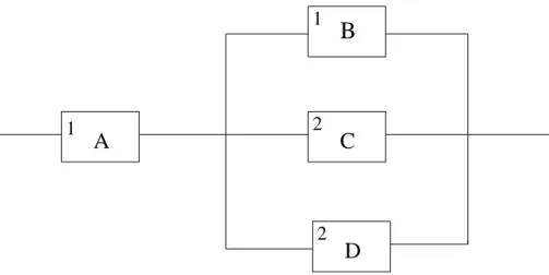
Example 2.2.1 Consider the system in Figure 2.1, which consists of four
compo-nents of two types, so m1 = m2 = 2. We want to examine the reliability of this
A
D
C
B
1 1 2 2Figure 2.1: System with four components of two types
l1 l2 Φ Φw 0 0 0 0 0 1 0 0 0 2 0 0 1 0 0 0 1 1 1/2 1 1 2 1/2 1 2 0 1 1 2 1 1 1 2 2 1 1
Table 2.1: Survival signatures for the system in Figure 2.1
swap only has a positive effect on the system reliability if component A fails while component B still functions and at least one of components C or D also still func-tions. So, the system’s structure function with this swap applied if needed, changes
from value 0 to 1 for three values of the state vectorx (with entries alphabetically
ordered): (0,1,0,1),(0,1,1,0),(0,1,1,1), as in these cases the failed component A
will be replaced by component B which is functioning, and indeed at least one more
component functions. The corresponding survival signatures, Φ (l1, l2) for the
sys-tem without the swap, and Φw(l
1, l2) with this specific swap applied if needed, are
given in Table 2.2 for all l1, l2 ∈ {0,1,2}.
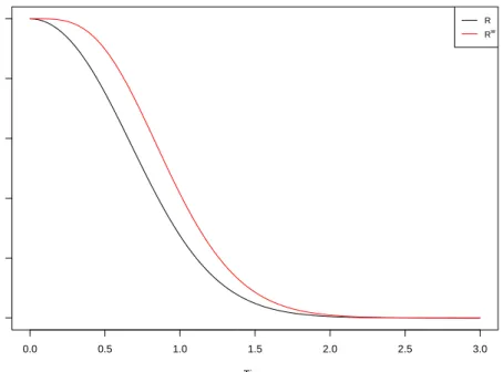
The reliability of the system without the swap being possible, and the reliability
0.0 0.5 1.0 1.5 2.0 2.5 3.0 0.0 0.2 0.4 0.6 0.8 1.0 Time Reliability R Rw
Figure 2.2: Reliability of system in Figure 2.1
and Φw(l
1, l2) by the probability that the number of components of each type will
be functioning, assuming independence of failure time of components of different types. Let the CDFs of the failure times of the Type 1 and Type 2 components be
F1(t) and F2(t), respectively. Then the reliability R(t) of the system without the
swap being possible, and the reliability Rw(t) of the system with the swap applied
if needed are
R(t) = [F1(t)][1−F1(t)][1−[F2(t)]2] + [1−F1(t)]2
Rw(t) = 2[F1(t)][1−F1(t)][1−[F2(t)]2] + [1−F1(t)]2 (2.2.4)
Figure 2.2 presents R(t) and Rw(t) if the failure times of Type 1 components
have a Weibull distribution with shape parameter 2 and scale parameter 1, that
is with CDF F1(t) = 1−e−t
2
, and the failure times of Type 2 components have
an Exponential distribution with expected value 1, so with CDF F2(t) = 1−e−t.
This figure clearly presents the gain in reliability of the system due to the possible component swap.
2 2
D
E
2C
B
1A
1Figure 2.3: System with five components of two types
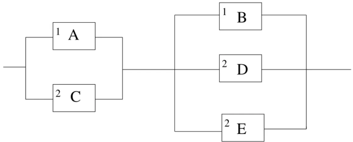
Example 2.2.2 Consider the system in Figure 2.3, which consists of five
com-ponents m = 5 with two types K = 2, so m1 = 2 and m2 = 3. We want to
examine the reliability of this system in the case that components A and B can be swapped. The system can benefit from this swap if components A and C are functioning while components B, D and E are failed and if components A and C are failed while component B and at least one of components D and E are function-ing. So, the system’s structure function with this swap applied, changes from value
0 to 1 for four values of the state vector x (with entries alphabetically ordered):
(1,0,1,0,0),(0,1,0,1,0),(0,1,0,0,1),(0,1,0,1,1). The survival signature, Φ (l1, l2)
for the system without the swap, and Φw(l
1, l2) with the swap applied, are given in
Table 2.2 for alll1 ∈ {0,1,2}and l2 ∈ {0,1,2,3}.
Let the probability distribution of the Type 1 components failure time have CDF
F1(t) and the probability distribution of the Type 2 components failure time have
CDFF2(t). Then the reliability of the systemR(t) without the swap being possible,
and the reliabilityRw(t) of the system with the swap applied if needed are
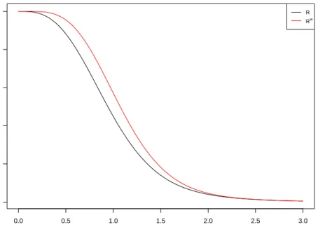
R(t) =[F1(t)]2 h 2[F2(t)][1−F2(t)]2 + [1−F2(t)]3 i + [F1(t)][1−F1(t)] h 3[F2(t)]2[1−F2(t)] + 5[F2(t)][1−F2(t)]2+ 2[1−F2(t)]3 i + [1−F1(t)]2. Rw(t) =[F1(t)]2 h 2[F2(t)][1−F2(t)]2+ [1−F2(t)]3 i + 2[F1(t)][1−F1(t)] h 1−[F2(t)]3 i + [1−F1(t)]2. (2.2.5)
l1 l2 Φ Φw 0 0 0 0 0 1 0 0 0 2 2/3 2/3 0 3 1 1 1 0 0 0 1 1 1/2 1 1 2 5/6 1 1 3 1 1 2 0 1 1 2 1 1 1 2 2 1 1 2 3 1 1
Table 2.2: Survival signatures for the system in Figure 2.3
If we keep the same scenario for the failure times of Type 1 and Type 2 com-ponents as in Example 2.2.1, we can see in Figure 2.4 how the system’s reliability change over time before and after the possible component swaps. It is clear that there would be a good improvement in the system’s reliability if the system is de-signed in the way that we could implement the defined swap.
It is clear from the previous example that the effect the swap between components A and B is fully taken into account through the system structure function, and hence the survival signature. This has the important advantage that each components remains of the same type when compared to the system without swaps being possible. This is not the case in the alternative approach as we will see.
2.2.1
Alternative approach
In this approach we consider the change that might happen in reliability of a system if its components can be swapped upon failure in the failure times of the specific locations that the system’s components fixed on. For example, for the system in
Figure 2.1, let us assume that LA, LB, LC and LD denote the locations in the
system that components A, B, C and D are fixed on, respectively. If a swap could
0.0 0.5 1.0 1.5 2.0 2.5 3.0 0.0 0.2 0.4 0.6 0.8 1.0 Time Reliability R Rw
Figure 2.4: Reliability of the system in Figure 2.3
time the maximum of the failure times of components A and B, and location LB
would have as failure time the minimum of the failure times of components A and B.
Hence, LA and LB would not have exchangeable failure times anymore, and hence
they would not be of the same type, so the swap breaks down these locations into two different types.
In order to consider the change that might happen in reliability in the failure times of the specific locations, we define the survival signature according to the
specific locations. Consider a system withm components. Let L1, L2,· · · , Lm
rep-resent different locations in the system that the components might be fixed on. TLj
denote the failure time of locationLj, j ∈ {1,2,· · · , m} and it represents the time
at which this location will contain a failed component. The survival signature of
specific locations gives the probability that system functions if there is exactlyYb of
typeb locations functioning. Assuming that the random failure times of locations of
the same type are exchangeable, while full independence is assumed for the random
failure times of locations of different types. If we haveB ≥2 types of locations with
functioning states of thej location of typeb. abj = 1 ifjth location of typebfunction
and ab
j = 0 if it fails. ab = ab1, ab2,· · · , abmb
is a state vector that represents the
state of type b locations and a = a1, a2,· · · , aB
is the state vector for the overall system. The structure function that gives the overall state of the system according
to the functioning status of specific locations is denoted by φL(a).
There are mbYb
state vectors ab with exactly Y
b of its mb locations abj = 1, so
with Pmb
j=1abj = Yb. We denote the set of these state vectors for locations of type
b by Sb
Y. Let SY1,...,YB denote the set of all state vectors for the whole system for
which Pmb
j=1abj =Yb, for b = 1,2, ..., B. Because of the assumption that the failure
times of mb locations of type b are exchangeable, all the state vectors ab ∈ SYb are
equally likely to occur. The survival signature of specific locations is denoted by ΦL(Y1, Y2,· · · , YB), and is given as follows:
ΦL(Y1, Y2,· · · , YB) = B Y b=1 mb Yb −1! × X a∈SY1,···,YB φ(a). (2.2.6)
To find the reliability of the system Rw(t) that considers a defined swap, we
find ΦL(Y1, Y2,· · · , YB) , then we multiply it by the probability that the number of
specific locations of each type will be functioning, taking into account the defined
swap in the failure time of specific locations. Let Nb
t ∈ {0,1, ..., mb} denote the
number of type b locations in the system that function at time t > 0. To find
P(N1
t = Y1, Nt2 = Y2,· · · , NtB = YB), we need to find the joint probability that
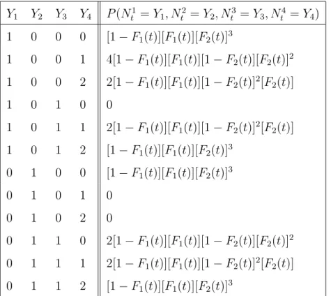
consider the dependency that occurred between specific locations as a result of the defined swap. Rw(t) = m1 X Y1=0 ... mB X YB=0 ΦL(Y1, Y2,· · · , YB)P(Nt1 =Y1, Nt2 =Y2,· · · , NtB=YB) (2.2.7) This approach is illustrated in more detail through the following two examples.
Example 2.2.3 Consider the same system in Figure 2.1 and the same swapping
possibility between components A and B as discussed in Example 2.2.1. The time
at which locationLAfails,TLA, is dependent on the time at which location LB fails,
TLB. TLA = max(TA, TB) and TLB = min(TA, TB) where TA is the failure time of
Y1 Y2 Y3 ΦL Y1 Y2 Y3 ΦL 0 0 0 0 1 0 0 0 0 0 1 0 1 0 1 1 0 0 2 0 1 0 2 1 0 1 0 0 1 1 0 1 0 1 1 0 1 1 1 1 0 1 2 0 1 1 2 1
Table 2.3: Survival signature ΦL of system in Figure 2.1
B with disregard to its location. It is clear that under the defined swap, LA and
LB represent two different types of locations. We have Y1 ∈ {0,1} corresponding
to locationLA and we have Y2 ∈ {0,1} corresponding to location LB. The defined
swap does not change the locations of Type 2 components, so all of the locations of Type 2 components still have the same type as its components we denote this Type
3 and we have Y3 ∈ {0,1,2}.
In order to find the reliability of the system, we calculate ΦL(Y1, Y2, Y3) with
disregard to the structure of components in the system. For example, in the
situ-ation that if locsitu-ationLA fails while locations LB, LC and LD are still functioning,
the structure function in this situation is φL(a11 = 0, a12 = 1, a31 = 1, a32 = 1) = 0,
comparing to the structure function φ(x11 = 0, x21 = 1, x21 = 1, x22 = 1) = 0 for the
original system,φLbreaks down the system locations to different types according to
the change that happens in their failure times as a result of the defined swap. Table
2.3 demonstrates ΦL for all Y1, Y2 ∈ {0,1} and Y3 ∈ {0,1,2}.
To find P(Nt1 = Y1, Nt2 = Y2, Nt3 = Y3) for all Y1, Y2 ∈ {0,1} and Y3 ∈ {0,1,2}.
We need to find the joint probability of P(N1
t =Y1, Nt2 =Y2) for all Y1, Y2 ∈ {0,1}
then multiply it by the probability that the number of locations of type 3 will be
functioning P(N3
t =Y3) because under the defined swap, Nt3 is still independent of
Nt1 and Nt2.
Components A and B are of the same type. So, TA and TB are identically
distributed TA, TB ∼ F1(t) where F1(t) is CDF of the failure time of Type 1
LB are functioning together at time t > 0 is P(Nt1 = 1, Nt2 = 1) = [1−F1(t)]2
and the probability that these two locations are not functioning at time t > 0 is
P(N1
t = 0, Nt2 = 0) = [F1(t)]2. The event that locationLA functions while location
LB is failed will occur when location LA contains functioning component A and
location LB contains a failed component B or when component A fails at location
LAand it was swapped with functioning component B. The probability of this event
is P(N1
t = 1, Nt2 = 0) = 2[F1(t)][1−F1(t)]. Also, it is impossible that location LB
functions while location LA fails. So, P(Nt1 = 0, Nt2 = 1) = 0. If we substitute the
values of ΦL and the joint probability in Equation (2.2.7), we can find that
Rw(t) = 2[F1(t)][1−F1(t)][1−[F2(t)]2] + [1−F1(t)]2 (2.2.8)
Comparing the results in Equations (2.2.4) and (2.2.8), we can clearly see that we arrived at the same result by implementing the two different approaches.
Example 2.2.4 Consider again the system in Figure 2.3 and the same swapping
possibility between the components A and B as discussed in Example 2.2.5. The
defined swap will only change the failure time of locations LA and LB in the
situations when the location LC functions while the locations LD and LE fail,
TLA = min(TA, TB) and TLB = max(TA, TB), and in the situation that the location
LC fails while at least one of the locationsLD and LE function,TLA = max(TA, TB)
andTLB = min(TA, TB). In the situation that the locationLC,LD andLE are
func-tioning together or failed together, the swap will not influence the failure time of
locationsLA and LB. Thus, they still have their original failure times in this
situa-tion,TLA =TAandTLB =TB. It clear that the failure timeTLA is not exchangeable
with the failure timeTLB. So, the locationsLAandLB represent two different types
namely Type 1 and Type 2 locations and we have Y1 ∈ {0,1} corresponding to the
number of Type 1 locations functioning and we have Y2 ∈ {0,1} corresponding to
the number of Type 2 locations functioning. SinceTLA and TLB dependent onTLC
and either one of TLD and TLE, we breakdown the location of Type 3 components
into two types, namely Type 3 location represents the locationLC and Type 4
rep-resents the location LD and LE. So, we have Y3 ∈ {0,1} and Y4 ∈ {0,1,2}. Table
Y1 Y2 Y3 Y4 ΦL Y1 Y2 Y3 Y4 ΦL 0 0 0 0 0 1 0 0 0 0 0 0 0 1 0 1 0 0 1 1 0 0 0 2 0 1 0 0 2 1 0 1 0 0 0 1 1 0 0 1 0 1 0 1 0 1 1 0 1 1 0 1 0 2 0 1 1 0 2 1 0 0 1 0 0 1 0 1 0 0 0 0 1 1 1 1 0 1 1 1 0 0 1 2 1 1 0 1 2 1 0 1 1 0 1 1 1 1 0 1 0 1 1 1 1 1 1 1 1 1 0 1 1 2 1 1 1 1 2 1
Table 2.4: Survival signature ΦL of system in Figure 2.3
Components A and B are of the same type. So, TA and TB are identically
dis-tributedTA, TB ∼F1(t) whereF1(t) is CDF of the failure time of Type 1 components.
Components C, D and E are of the same type. So,TC,TD andTE are identically
dis-tributedTC, TD, TE ∼F2(t) whereF2(t) is CDF of the failure time of Type 2
compo-nents. It is clear that the joint probability P(Nt1 =Y1, Nt2 =Y2, Nt3 =Y3, Nt4 =Y4)
would be different than the joint probability for the original system only in the
situations when Nt1 = 1 and Nt2 = 0 or when Nt1 = 0 and Nt2 = 1. For example,
P(N1
t = 1, Nt2 = 0, Nt3 = 0, Nt4 = 1) = 4[1−F1(t)][F1(t)][1−F2(t)][F2(t)]2 because
the event that LA and one of LD or LE function while LB and LC are failed will
occur in 4 situations namely, when LA contains functioning component A and LD
contains functioning component D and LB, LC and LE contain failed components,
or whenLAcontains functioning component A and LE contains functioning
compo-nent E andLB,LC andLD contain failed components, or when component A fails at
LAand it is swapped by the functioning component B and LD contains functioning
component D and LB, LC and LE contain failed components, or when component
Y1 Y2 Y3 Y4 P(Nt1 =Y1, Nt2 =Y2, Nt3 =Y3, Nt4 =Y4) 1 0 0 0 [1−F1(t)][F1(t)][F2(t)]3 1 0 0 1 4[1−F1(t)][F1(t)][1−F2(t)][F2(t)]2 1 0 0 2 2[1−F1(t)][F1(t)][1−F2(t)]2[F2(t)] 1 0 1 0 0 1 0 1 1 2[1−F1(t)][F1(t)][1−F2(t)]2[F2(t)] 1 0 1 2 [1−F1(t)][F1(t)][F2(t)]3 0 1 0 0 [1−F1(t)][F1(t)][F2(t)]3 0 1 0 1 0 0 1 0 2 0 0 1 1 0 2[1−F1(t)][F1(t)][1−F2(t)][F2(t)]2 0 1 1 1 2[1−F1(t)][F1(t)][1−F2(t)]2[F2(t)] 0 1 1 2 [1−F1(t)][F1(t)][F2(t)]3
Table 2.5: The probability in the cases when N1
t = 1 and Nt2 = 0 and in the cases
whenN1
t = 0 and Nt2 = 1 in Example 2.2.4
contains functioning component C and LB, LC and LD contain failed component.
Table 2.5 shows P(N1
t =Y1, Nt2 =Y2, Nt3 =Y3, Nt4 =Y4) in the cases when Nt1 = 1
and Nt2 = 0 and in the cases when Nt1 = 0 and Nt2 = 1 , for all Y3 ∈ {0,1} and
Y4 ∈ {0,1,2}.
By substituting the values of ΦL(Y1, Y2, Y3, Y4) and P(Nt1 = Y1, Nt2 =Y2, Nt3 =
Y3, Nt4 =Y4) for all Y1, Y2, Y3 ∈ {0,1} and Y4 ∈ {0,1,2} in Equation(2.2.7), we can
find that Rw(t) =[F1(t)]2 h 2[F2(t)][1−F2(t)]2+ [1−F2(t)]3 i + 2[F1(t)][1−F1(t)] h 1−[F2(t)]3 i + [1−F1(t)]2. (2.2.9)
Therefore, we arrived at the same result as in Example 2.2.2. It clear from the previous examples that while we arrived at the same result by implementing the two different approaches. The first approach in which the effect of a defined swapping regime is fully taken into account through the system structure function,
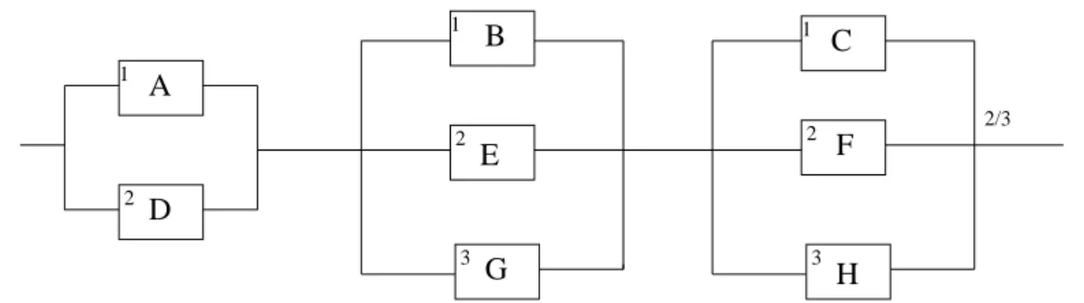
A B C D E G H F 3 3 1 2 1 2 2 1 2/3
Figure 2.5: System with 8 components of 3 types; C,F,H form a 2-out-of-3 subsystem
and hence the survival signature is more attractive than the second one, since it has continued with the same advantage of survival signature by modeling the structure of systems and separating it from the random failure time of components. However, in the second approach in which the effect of such a component swap is taken into account through the failure times of specific locations, the lifetime distributions become extremely complex and may not be feasible if one has a variety of swapping opportunities. This thesis considers only the first approach for reliability assessment when system components can be swapped.
The following extensive example is comparing the change that might happen in the reliability as a result of different swapping opportunities. We can see through this example how the reliability of the system can be obtained easily by considering the first approach, however it would be quite difficult to obtain it by the second approach.
Example 2.2.5 The system in Figure 2.5 consists of 8 components of 3 types,
m = 8 and K = 3, m1 = 3, m2 = 3 and m3 = 2. The letters A to H represent
the specific components, the numbers 1 to 3 represent the component types. This system consist of three subsystems in series configuration. The first subsystem is a parallel system consisting of components A and D, the second subsystem is a parallel system consisting of components B, E and G, and the third subsystem is a 2-out-of-3 system consisting of components C, F and H.
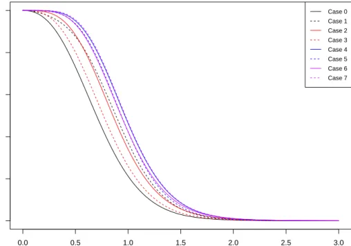
The reliability of this system might be enhanced by a variety of swapping op-portunities, we compare 7 swapping cases. In Case 1, we assume that we are able to swap only Type 1 components, in Case 2, we assume that we are able to swap
only Type 2 components, in Case 3, we assume that we are able to swap only Type 3 components, in Case 4, we assume that we are able to swap both Type 1 and Type 2 components, in Case 5, we assume that we are able to swap both Type 1 and Type 3 components, in Case 6, we assume that we are able to swap both Type 2 and Type 3 components, in Case 7, we assume that we are able to swap Type 1, Type 2 and Type 3 components. In each case the swap can be done in any way when needed to keep the system functioning.
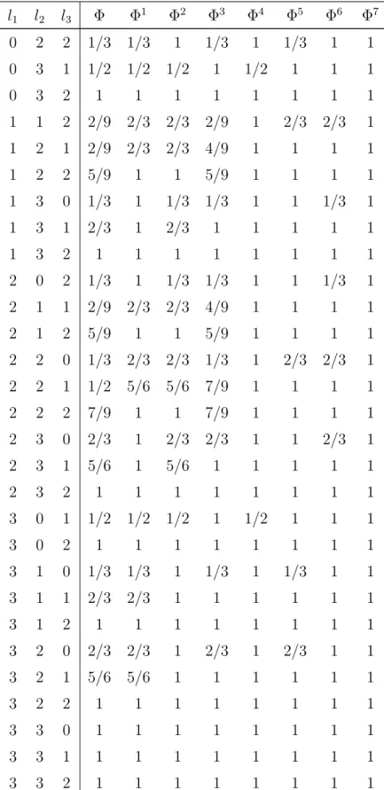
The survival signatures are given in Table 2.6, where Φ is the survival signature
for the original system and Φw, w ∈ {1,2,3,4,5,6,7} are the survival signatures in
Cases 1, 2, 3, 4, 5, 6 and 7. In this table we present only nonzero values. The zero values represent the situations when the system has only 3 functioning components or less, because the system needs at least 4 components to function. In Case 7, all nonzero values are equal to 1, because in this case we can swap components of all types, so the system just needs four functioning components of any type in order to function.
In order to see the change to the system’s reliability as a result of each of swap-ping case, we assume that the failure times of Type 1 components have a Weibull distribution with shape parameter 2 and scale parameter 1, the failure times of Type 2 components have an Exponential distribution with expected value 1 and the failure times of Type 3 components have an Exponential distribution with expected
value 2, soF1(t) = 1−e−t
2
, F2(t) = 1−e−t and F3(t) = 1−e−t/2. The reliability
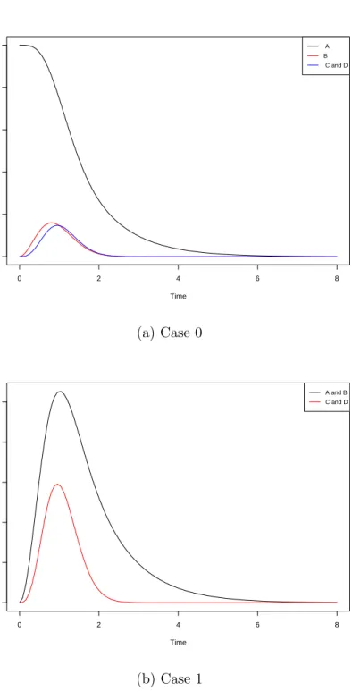
functions of the system in Cases 1, 2, 3, 4, 5, 6 and 7 are given in Figure 2.6. Case 0 in this figure represents the reliability function for the original system. Clearly, while all swap cases would enhance the system reliability, Cases 7 and 4 provide the best improvement, which is mainly due to the fact that in Case 7 all the components are involved in the swaps and in Case 4, six components are involved in the swaps, including the two components in the first subsystem.
l1 l2 l3 Φ Φ1 Φ2 Φ3 Φ4 Φ5 Φ6 Φ7 0 2 2 1/3 1/3 1 1/3 1 1/3 1 1 0 3 1 1/2 1/2 1/2 1 1/2 1 1 1 0 3 2 1 1 1 1 1 1 1 1 1 1 2 2/9 2/3 2/3 2/9 1 2/3 2/3 1 1 2 1 2/9 2/3 2/3 4/9 1 1 1 1 1 2 2 5/9 1 1 5/9 1 1 1 1 1 3 0 1/3 1 1/3 1/3 1 1 1/3 1 1 3 1 2/3 1 2/3 1 1 1 1 1 1 3 2 1 1 1 1 1 1 1 1 2 0 2 1/3 1 1/3 1/3 1 1 1/3 1 2 1 1 2/9 2/3 2/3 4/9 1 1 1 1 2 1 2 5/9 1 1 5/9 1 1 1 1 2 2 0 1/3 2/3 2/3 1/3 1 2/3 2/3 1 2 2 1 1/2 5/6 5/6 7/9 1 1 1 1 2 2 2 7/9 1 1 7/9 1 1 1 1 2 3 0 2/3 1 2/3 2/3 1 1 2/3 1 2 3 1 5/6 1 5/6 1 1 1 1 1 2 3 2 1 1 1 1 1 1 1 1 3 0 1 1/2 1/2 1/2 1 1/2 1 1 1 3 0 2 1 1 1 1 1 1 1 1 3 1 0 1/3 1/3 1 1/3 1 1/3 1 1 3 1 1 2/3 2/3 1 1 1 1 1 1 3 1 2 1 1 1 1 1 1 1 1 3 2 0 2/3 2/3 1 2/3 1 2/3 1 1 3 2 1 5/6 5/6 1 1 1 1 1 1 3 2 2 1 1 1 1 1 1 1 1 3 3 0 1 1 1 1 1 1 1 1 3 3 1 1 1 1 1 1 1 1 1 3 3 2 1 1 1 1 1 1 1 1