ModelMage: A TOOL FOR AUTOMATIC MODEL GENERATION, SELECTION AND MANAGEMENT

ModelMage: A TOOL FOR AUTOMATIC MODEL GENERATION, SELECTION AND MANAGEMENT

MAX FL ¨OTTMANN1 _{J ¨ORG SCHABER}1 _{STEPHAN HOOPS}2 [email protected] [email protected] [email protected]

EDDA KLIPP1 _{PEDRO MENDES}2,3 [email protected] [email protected]

1_{Max-Planck-Institute for Molecular Genetics, Ihnestr 63-73, 14195 Berlin, Germany} 2_{Virginia Bioinformatics Institute - 0477, Virginia Tech, Bioinformatics Facility I,}

Blacksburg, Va 24061, USA

3_{The University of Manchester, 131 Princess Street, Manchester M1 7DN, United}

Kingdom

Mathematical modeling of biological systems usually involves implementing, simulating, and discriminating several candidate models that represent alternative hypotheses. Gen-erating and managing these candidate models is a tedious and difficult task and can easily lead to errors. ModelMage is a tool that facilitates management of candidate models. It is designed for the easy and rapid development, generation, simulation, and discrim-ination of candidate models. The main idea of the program is to automatically create a defined set of model alternatives from a single master model. The user provides only one SBML-model and a set of directives from which the candidate models are created by leaving out species, modifiers or reactions. After generating models the software can au-tomatically fit all these models to the data and provides a ranking for model selection, in case data is available. In contrast to other model generation programs, ModelMage aims at generating only a limited set of models that the user can precisely define. ModelMage uses COPASI as a simulation and optimization engine. Thus, all simulation and opti-mization features of COPASI are readily incorporated. ModelMage can be downloaded fromhttp://sysbio.molgen.mpg.de/modelmage and is distributed as free software. Keywords: model families; systems biology; model discrimination; candidate model; model simulation; model generation

1. Introduction

It has been recognized that despite the increasing amount and accuracy of molecular biological data, uncertainty about biochemical network structures and dynamics is still immense. The uncertainty is not only limited to different parameter sets, but also affects structure and kinetics of models [1]. This naturally prompts alterna-tive hypotheses about biological processes, which directly translate into alternaalterna-tive mathematical model formulations.

Generating and handling alternative model formulations poses a considerable challenge to the modeler for several reasons. First, each model has to be imple-mented, simulated and analyzed separately. Often, model alternatives vary only

slightly in structure and kinetics [2], which seduces the modeler to copy the original model and then introduce the modifications by hand. This is an error-prone pro-cess. Secondly, changes that affect the whole family of models have to be updated in each model separately, which is also error-prone and a tedious task, especially when the number of models is high. Biological models with many uncertainties often lead to a very high number of possible alternatives, because of combinatorial complex-ity, which renders it impossible to implement and handle each model individually. Under these conditions keeping track of changes in models is also a hard task.

The above mentioned problems resulted in the development of several formalisms and tools that address these problems. In addition to model building and analysis tools like Copasi [3] or Celldesigner [4], there are a number of tools that specifically deal with uncertainties in model building [5–7].

These state-of-the-art approaches have a major short-coming. Even though most tools aim at handling combinatorial complexity, they produce only one model at the end, which includes all or a reduced number of possible molecular interactions generated from certain rules. As an alternative, we present a tool that automatically implements and manages a set of models, which differ in the number of species, reactions or kinetics, because this is what modelers in systems biology usually are confronted with. MMT2 [8] is a tool that aims into that direction but it falls short in the ability to actually control the number and structure of generated models, because it produces all combinatorial possible alternatives.

In our daily work and in discussions with the community [9] we see that it is not so much the combinatorial complexity that poses problems for the modelers but rather to create and handle a specific set of candidate models that represent alternative formulation of biological processes. Often modelers have a very clear idea what different versions of a model they want to test. It is just too tiresome and error-prone to do this by hand, and this way good models may be omitted because of a lack of time.

ModelMage provides modelers with a tool that facilitates managing a set of candidate models. In the following we describe the main idea and the technology of ModelMage. Finally, we also provide a simple example of its usage.

1.1. The Idea

ModelMage automatically generates models based on a master model and certain directives that specify how candidate models are to be derived from the master model. Such candidate models are created by two basic processes, first, by removing species, modifiers or reactions from the master model and, second, by generating certain alternative kinetics for specified reactions.

The generated candidate models are automatically documented in a way that it is always comprehensible how they were derived from the master model, thereby keeping track of model versions. The principle of generating candidate models by leaving out components of a master model implies that the master model must

comprise all components of the candidate models.

The user has to provide only the structure of the master model, with or without kinetics, and directives for ModelMage. When no initial kinetics are assigned, Mod-elMage assumes mass action kinetics of appropriate order by default. There is no need to edit the individual models at any time. Thereby common parameters, mod-ifications or directives are changed in one place only and are automatically updated in each candidate model. This removes the errors introduced by modifying each model individually. Finally, all models are simulated, fitted to data and compared automatically, if data is available. At the end, the user is provided with a ranking of the model fits and statistical measures that help to discriminate between model alternatives. Command Line Reduction Directives SBML | Copasi Child Model SBML | Copasi Child Model SBML | Copasi Child Model SBML | Copasi Child Model SBML | Copasi Child Model SBML | Copasi Child Models Command Line Model Ranking SBML | Copasi Child Model C 1. SBML | Copasi Child Model A 2. SBML | Copasi Child Model D 3. SBML | Copasi Child Model B 4. SBML | Copasi Child Model E 5. ModelMage Generator ModelMage Discriminator CopasiUI Parameter Estimation Task CopasiSE Parameter Estimation SBML | Copasi Master Model S re2 re3 re11 re3 re5 re6 re7 re12 x1 x2 x3 x4 x5 r u

Fig. 1. Workflow of ModelMage.

2. Methods

2.1. Generating Alternative Models

Generation of candidate models in ModelMage is a two step process. The first step is to create a master model in Copasi or in any other SBML [10, 11] compliant editor like CellDesigner [4] or Semantic SBML [12]. This model must include all possible species and reactions that shall be included in at least one of the alternative models. In the second step the set of candidate models is built by removing reactions, species or modifiers from the master model. (Fig. 1)

The removal and exchange is done by giving simple directives to the program as command line parameters. There are two parameters that can be specified to generate alternatives (Table 1). The parameter --kinetics is used to exchange the kinetic law in the specified reactions. This can be achieved by a simple syntax without typing the whole formula and with default values for parameters. The user has to choose the reaction and to give ModelMage a short form of the kinetics that shall be passed to it i.e.re 2(MM)would set reaction re 2 to Michaelis-Menten kinetics in one candidate model if the number of reactants and modifiers is suitable. At the moment, only mass action (MA) and Michaelis-Menten (MM) kinetics can

Parameter Values Function

-r, --remove logical combinations of

species and reactions, e.g.

species 1 & reaction 2

defines which

species,reactions or mod-ifiers should be removed from the master model

-k, --kinetics X(MA | MM) change the kinetics of

re-action X to mass

ac-tion (MA) or Michaelis-Menten (MM)

-d, --discriminate RSS, AIC AICc AICc is

default

Run a parameter estima-tion in COPASI and rank the models by the selected criterium.

-o, --output path/filename Path and basic filename

for the output files. Mod-elMage will add identifiers to the created models and create the subdirectories

ResultSBMLFiles and

ResultCopasiFiles

-v, --verbose no arguments Returns

more detailed command line output about the cre-ated models.

be set by using this parameter.

The SBML structure is not easy to work with internally, so the first step in the internal generation process is the conversion of the master model to a bipartide graph with one set of nodes for the reactions and the other set of nodes for the species.

To create the network structures of the candidate models one can use the

--removeparameter. The values of this parameter can be all possible logical

combi-nations of species, modifiers and reactions that should be removed from the master model to generate the candidate models.

2.1.1. Removing Reactions and Modifiers

Executing the command-r reaction identifier, ModelMage removes the speci-fied reaction from the model and leaves the connected species untouched. Removing reactions is fairly simple, because these can simply be deleted from the model and the worst effect can be two or more unconnected networks in the model. If the re-moval of a reaction results in unconnected subgraphs ModelMage by default prints

out a warning, but nevertheless removes the reaction.

The second graph entity that can be removed in ModelMage is the property of a component as a modifier in reactions. This is represented as an edge from the species to the reaction in the graph structure. Modifiers are also removed using the -r option. Removing the species as a modifier is invoked by a colon between both identifiers (e.g.-r species identifier:reaction identifier). In this case the modifiers of the specified reaction is removed, and the kinetics are changed to mass action kinetics of appropriate order to make sure that ModelMage generates a working model. re3

E

S

P

S

T

P

S

P

re1 re2 A B C D AB re3 A B C D A B C

Fig. 2. Examples of removed species. (A)Removal of an intermediate species. Species T is removed and reactions r1 and r2 are combined. (B) When an enzyme-substrate-complex is removed from a reaction ModelMage creates a new reaction with the enzyme set as a modifier. (C) Removal of species AB leads to new a reaction that is a combination of all incoming and outgoing reactions of the removed species.

2.1.2. Removing Species

When the user specifies a species for removal, ModelMage analyzes the neighbor-hood of this species and rewires the model in an intelligent manner. The rewiring heuristic follows the principle of reachability and it works the following way:

First, ModelMage detects the incoming and outgoing reactions of the species that shall be removed and analyses the species involved in these reactions, i.e. the substrates of which the removed species was the product and the products of which the removed species was the substrate (see Fig. 2). Then, ModelMage tries to combine all pairs of incoming and outgoing reactions into one single new reaction. The new reaction inherits all substrates and products from the combined reactions and assigns a kinetic for the new reaction. The inserted kinetic can either

be the kinetics of the ancestors if they were equal and are still suitable for the combined reaction, or mass action otherwise. There are three possible cases for each combination of incoming and outgoing reactions that have to be considered and treated separately.

(1) If the combination of a pair of incoming and outgoing reactions would result in reaction, which has the same species, both as substrates and as products, i.e. a self loop to a list of species, the respective reactions are not combined.

(2) If there is only a subset of species equal in both substrates and products, then these species are regarded as enzymes and are set as a modifiers for the resulting reaction (Fig. 2 B).

(3) If the sets are disjunct then the reactions are combined in the above described way.

The main algorithm to remove one species looks like this: def remove ( s ) : f o r i in s . i n c o m i n g R e a c t i o n s : f o r o in s . o u t g o i n g R e a c t i o n s : i f i == o : s e l f L o o p ( i , o ) e l s e i f i p a r t i a l l y E q u a l o : s u b s t r a t e E n z y m e ( i , o ) e l s e: combine ( i , o ) del( i , o ) del( s )

As mentioned before, removing combinations of species and reactions can lead to large numbers of candidate models. The user has to be careful how many com-ponents are combined for removal, because there is the danger of combinatorial explosion, especially if the components are combined by OR operators (Fig. 3). Exchanging kinetics also increases the number of models, because every structural model is generated with every possible set of kinetics.

To simplify the process of finding the right logical formulations to create cer-tain model families, the user can specify different sets of models in one sin-gle run of ModelMage. This can be achieved by concatenating different logical formulas by ’,’ i.e. ModelMage.py -r (species 1 ^ species 2),(reaction 4 &

reaction 1) example.cps. This would generate three new alternative models. Two

are generated from the first bracket, where in one species 1 and in the other

species 2is removed. The third model is generated from the second bracket, where

both reactions are removed from the model.

2.2. Model Discrimination

When data for certain components is available, ModelMage can select the best model from the generated model family. ModelMage can automatically fit the mod-els to the data by estimating parameters and is able to rank the modmod-els by different

A

C

B

E

D

A

B

C

D

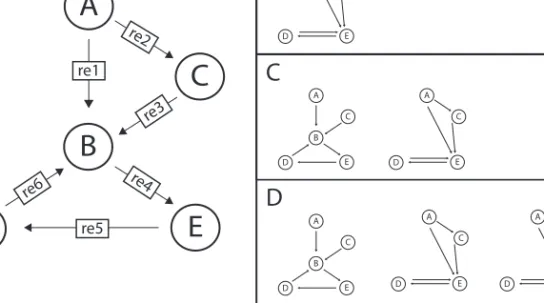
Fig. 3. Logical combinations of alternative models. (A) Master Model from which the alternatives can be generated by ModelMage.(B)One model is generated by the logical string ”B & re 2”. The logical AND means that species B and reaction re 2 must both be removed in this model.(C)The XOR in the command ”B ^ re 2” produces two models, because in each of them only one node is removed.(D)The OR operator ”B | re 2” creates a combination of B and C

statistical measures to determine the best model. For parameter estimation Model-Mage utilizes Copasi’s various parameter estimation routines, which makes it very fast and flexible. The parameter estimation task is most conveniently defined in Co-pasi’s graphical user interface and can later be executed by ModelMage. The user has to set up the task only once for the master model. ModelMage automatically defines the parameter estimation task for all generated candidate models. Parame-ters of new or changed reactions are added to the estimation task if the parameParame-ters of the original reactions were part of the parameters estimation task of the master model. If there are parameters that do not exist in the specific alternative model they are deleted from the estimation task for this model.

The parameter estimation in Copasi creates output files for all of the models that contain details about the results of the estimation. ModelMage parses these files and extracts the objective value, which is the sum of weighted squared residuals of the fitted model (RSS). From this, e.g., the Akaike Information Criterion [13] is calculated for each model:

AIC= 2k+n(ln(RSS/n) + 1), (1)

where n is the number of observations and k is the number of estimated pa-rameters, which are also parsed from the Copasi output. From the AIC we can also compute the second order AIC (AICc):

AICc=AIC+2k·(k+ 1)

n−k−1 (2)

The AICc is used as the standard measure for ranking and model selection in ModelMage. The lower the AICc the better is the fit to the data and the higher is the ranking the model gets. AICc corrects the AIC for small number of observations, which is common in systems biology. But it can be also employed with bigger samples, because it converges to AIC when big sample sizes are available. [14, 15]

2.3. Implementation

We use SBML and libSBML because it is accepted as standard for exchange of models between systems biology tools. [9, 16] We decided to develop ModelMage closely related to Copasi because it is widely used in the community to work with dynamical models and has a rich set of features to build upon. ModelMage is written in Python, which makes it very flexible and portable to many platforms. Currently, it is tested on Linux, Mac OS and Windows. Parameter estimation is done by the fast Copasi algorithms. The rest of ModelMage’s features are not computationally intense which justifies the use of an interpreted language like Python for the tool. To install and run ModelMage, a system must meet the following requirements:

• Python≥2.5

• Networkx package for Python

• libSBML 3.0.1≥[17]

• Copasi≥4.2

3. Results and Discussion 3.1. Example

To verify ModelMage’s functionality we created a small master model that resembles a signaling cascade that includes three hypothetical feedback loops. (Fig. 4) From one alternative model we generated time-series data by simulating the model for 80 time units and sampled the values of species S, X5 and X6 at 7 time points. To get a more realistic test case we introduced small normally distributed errors into the data. After that, we used ModelMage to generate a family of ten models from the master model and fitted every model to the artificial data in a blind test. i.e. the person who used ModelMage did not know the model that produced the data beforehand. The model that produced the data was correctly recovered by the discrimination procedure of ModelMage.

The fits were done only for parameters of the reactions re3, re10, re11 and re12. The rest of the parameters were set to 0.1 to reduce the number of estimated parameters. For the parameter estimation we used the ”Evolutionary Programming” algorithm in Copasi and ranked the models by AICc. Results are shown in table 2.

S

X1

X2

X3

X4

X5

X6

u

The dashed lines were our hypotheses about feedbacks that possibly regulate the production ofr. ModelMage was started with the parameters -r ’re11, re11:X5 & re11:X6 , X4 & re11:X5 & re11:X6 , re11:X6 & re3:X6 , re11:X6

& re3:X6 & X4 , re11:X5 & re3:X6 , re11:X5 & re3:X6 & X4 ’ -k "re11(MM)" and produced all possible candidate models with different kinetics for re11 where possible. All these alterna-tives were also created with a double or single phosphorylation. Additionally one model with re11 completely removed was created.

# Model Objective Value AIC AICc n k

1. re11:X5 & re3:X6 & X4 0.0731 -46.9367 -44.9367 21 4

2. re11:X5 & re11:X6 & X4 0.1246 -33.7391 -29.7391 21 5 3. re11:X5 & re11:X6 & X4 0.1621 -30.2117 -28.2117 21 4

4. re3:X6 & re11:X6 & X4 0.1833 -27.6309 -25.6309 21 4

5. master model 1.3734 14.6623 16.6623 21 4

6. re11:X5 & re11:X6 1.6720 18.7939 20.7939 21 4

7. re11:X5 & re3:X6 1.6841 18.9455 20.9455 21 4

8. re3:X6 & re11:X6 1.7246 19.4449 21.4449 21 4

9. re11:X5 & re11:X6 1.5689 19.4577 23.4577 21 5

10. re11 4.4530 37.3652 37.3652 21 3

The ranking of candidate models clearly divided the models into 3 separate groups. The first group consists of the models which did not include species X4. They had objective values that were about 10 times smaller than those of the second group while fitting the same number of parameters. This also leads to big differences in the AICc. From this group the first ranking model, has a big difference to the following 3 models which all have very similar AICcs. This model is the one the data was created with.

The second group includes all the models that still include species X4 and rep-resent different ways of feedback. The master model, which was also fitted, ranked highest in this group, which is probably due the fact that it has all feedbacks still included and therefore can better regulate concentration of X6 then all the other models. Because of this obvious classification we did time course simulations for the best candidate model and the one that ranked seventh place. These models are very similar, the only difference is that the first ranking model contains X4 and the other one does not (Fig. 5).

The third group consists of the model where reaction re11 is completely removed, which has the worst fit of all the models. The bad fit is mainly due to the missing degradation of S. The other curves in this model also fit quite well, because there is still one feedback that can regulate X5 and X6 quite well.

0 20 40 60 80 0 0.2 0.4 0.6 0.8 1 1.2 t t t S 0 20 40 60 80 0 0.5 1 1.5 X5 0 20 40 60 80 0 1 2 3 4 5 X6

Fig. 5. Plots of simulations with the fitted models.(A)The signal is fitted similarly by models from both groups. (B) The lower ranking models do not reach the high amplitude in the X5 concentration.(C)The concentrations of X6 reach a maximum and decay after 70s in the model from the second group, whereas they reach a limit in the model from the first group. This difference can be seen in all the models.

3.2. Conclusions

The software we developed can substantially facilitate and accelerate the genera-tion and discriminagenera-tion of model alternatives. Model families can be created, ana-lyzed and changed far easier than it was possible before. The generated models are portable to any other SBML compliant software, which gives the user the possibil-ity to view and analyze them with an array of already existing tools. Our example model could be generated and clearly be recovered from a family of slightly different models in a very short time.

To use Modelmage it must be installed locally and can be downloaded from

http://sysbio.molgen.mpg.de/modelmage, but it would be possible to create a web-based version of the generator to make it easier to use.

The ranking criteria worked well despite a limited set of data to fit. If this is also the case in real biological examples remains to be investigated. Nevertheless

the user has to be careful when selecting models and the ranking by AIC should only be used as a hint to which might be the best model [8].

The most complicated step in using ModelMage is the formulation of the logical combination of removals, which can become quite difficult in some cases. We hope to improve this by adding a more sophisticated user-interface to ModelMage in upcoming versions. We are also planning to integrate a broader set of exchangeable kinetics to give the user more possibilities for alternatives.

Acknowledgements

MF was supported by the Max Planck Society and the German Academic Exchange Service (DAAD). JS was supported by the European Commision (QUASI (Contract No. 503230) and CELLCOMPUT (Contract No. 043310) and the DAAD.

References

[1] Kuepfer, L., Peter, M., Sauer, U., Stelling, J., Ensemble modeling for analysis of cell signaling dynamics,Nat Biotechnol, 25: 1001–10066, 2007.

[2] Geva-Zatorsky, N., Rosenfeld, N., Itzkovitz, S., Milo, R., Sigal, A., Dekel, E., Yarnitzky, T., Liron, Y., Polak, P., Lahav, G., Alon, U., Oscillations and variabil-ity in the p53 system,Mol Syst Biol, 2:0033, 2006.

[3] Hoops, S., Sahle, S., Gauges, R., Lee, C., Pahle, J., Simus, N., Singhal, M., Xu, L., Mendes, P., Kummer, U., COPASI–a complex pathway simulator, Bioinformatics, 22(24): 3067-30-74, 2006.

[4] Funahashi, A., Morohashi, M., Kitano, H., and Tanimura, N., Celldesigner: a process diagram editor for gene-regulatory and biochemical networks,Biosilico, 1: 159–162, 2003.

[5] Shapiro, B.E., Levchenko, A., Meyerowitz, E.M., Wold, B.J., Mjolsness, E.D., Celler-ator: extending a computer algebra system to include biochemical arrows for signal transduction simulationsBioinformatics, 19(5): 677–678, 2003.

[6] Blinov, M.L., Faeder, J.R., Goldstein, B., Hlavacek, W.S., BioNetGen: software for rule-based modeling of signal transduction based on the interactions of molecular domains,Bioinformatics, 20(17): 3289–3291, 2004.

[7] Lok, L. and Brent, R., Automatic generation of cellular reaction networks with mole-culizer 1.0.,Nat Biotechnol, 23(1): 131–136, 2005.

[8] M. Haunschild, B. Freisleben, R. Takors and W. Wiechert, Investigating the dynamic behavior of biochemical networks using model families,Bioinformatics, 21(8): 1617– 1625, 2005.

[9] Klipp, E., Liebermeister, W., Helbig, A., Kowald, A., and Schaber, J., Systems biology standards–the community speaks,Nat Biotechnol, 25: 390–391, 2007.

[10] Finney, A. and Hucka, M., Systems biology markup language: Level 2 and beyond,

Biochem Soc Trans, 31: 1472–1473, 2003.

[11] Hucka, M., Finney, A., Sauro, H. M., Bolouri, H., Doyle, J. C., Kitano, H., Arkin, A. P., Bornstein, B. J., Bray, D., Cornish-Bowden, A., et al., The systems biology markup language (SBML): a medium for representation and exchange of biochemical network models,Bioinformatics, 19: 524–531, 2003.

[12] Schulz, M., Uhlendorf, J., Klipp, E., and Liebermeister, W., SBMLmerge, a system for combining biochemical network models,Genome Inform,17(1): 62–71, 2006.

[13] Akaike, H., Information theory and an extension of the maximum likelihood principle,

Selected Papers of Hirotugu Akaike, 1998.

[14] Wagenmakers, E.-J. and Farrell, S., AIC model selection using Akaike weights,

Psy-chon Bull Rev, 11: 192–196, 2004.

[15] Burnham, K. and Anderson, D.,Model Selection and Multimodel Inference: A

Prac-tical Information-Theoretic Approach, Springer, 2002.

[16] Kell, D. B. and Mendes, P., The markup is the model: Reasoning about systems biology models in the semantic web era,J Theor Biol, 252(3): 538–543, 2008. [17] Bornstein, B. J., Keating, S. M., Jouraku, A., and Hucka, M., LibSBML: An API