c
SEMI-PARAMETRIC MODELS FOR RESPONSE TIMES AND RESPONSE
ACCURACY IN COMPUTERIZED TESTING
BY
CHUN WANG
DISSERTATION
Submitted in partial fulfillment of the requirements
for the degree of Doctor of Philosophy in Psychology
in the Graduate College of the
University of Illinois at Urbana-Champaign, 2012
Urbana, Illinois
Doctoral Committee:
Professor Hua-Hua Chang
Professor Jeff Douglas
Professor Lawrence J. Hubert
Professor Carolyn Anderson
Professor Jinming Zhang
Abstract
In computer-administered tests, response times can be recorded conjointly with the corresponding responses. This broadens the scope of potential modeling approaches because response times can be analyzed in addi-tion to analyzing the responses themselves. Current models for response times, however, mainly focus on parametric models that have the advantage of conciseness, but may suffer from a reduced flexibility to fit real data. This thesis presents two types of semi-parametric models that combine the flexibility of nonparametric modeling and the brevity as well as interpretability of the parametric modeling. They are
1. Hierarchical proportional hazard model: This model adopts the hierarchical structure suggested by van der Linden (2007) with the well-known Cox proportional hazard (PH) model in survival analysis. The PH model is comprised of two parts: the non-parametric baseline hazard and the parametric form of the examinee’s latent speed. This model acts on the hazard rate, the instantaneous rate at which the event occurs conditioning on the fact that the event has not occurred so far, and it assumes that a unit increase in a latent speed is multiplicative with respect to the hazard rate. The model includes the exponential regression model, Weibull regression model, and many other parametric models as special cases.
2. Hierarchical linear transformation model: This model is a further extension of the Cox PH model. In this model, the response times, after some non-parametric monotone transformation, become a linear model with latent speed as a covariate plus an error term. The distribution of the error term implicitly defines the relationship between the RT and examinees’ latent speeds; whereas the non-parametric transformation is able to describe various shapes of RT distributions. The linear transformation model represents a rich family of models that includes the Cox proportional hazard model, the Box-Cox normal model, and many other models as special cases. The linear transformation model is again embedded in a hierarchical framework so that both RTs and responses are modeled simultaneously. For both new models, we propose two-stage estimation methods. The model checking techniques for both models are provided to help practitioners decide whether the model is appropriate for a real data set.
Finally, the applicability of the new models are demonstrated with simulation studies and applications to actual responses to items.
Acknowledgments
This work was made possible through the support of many people. Special thanks to my adviser Professor Hua-Hua Chang for his guidance throughout my graduate study. I have benefited tremendously from his insight and knowledge. He has taught me everything from writing research papers, dealing with hard review comments, drafting proposals, to communicating with people friendly and professionally. He is not only a great mentor, but also one of my closest friends in life. There is no way that I could grow so much without his help and support. Also, thanks to Professor Jeff Douglas, who has provided countless hours of assistance and guidance throughout my dissertation work. His warm personality and kind encouragements have made the journey of my Ph.D. education a pleasure. I would also like to thank Professors Larry Hubert, Carolyn Anderson, and Jinming Zhang, whose lectures and lessons form the cornerstone of my statistical and ethical training as a quantitative psychologist.
Special thanks to my beloved parents and sister, thank you so much for raising me for the past twenty six years, giving me strongest support and walking me through various difficulties in my life. I can never come so close to my dream without you. I also want to express my sincere thanks to my husband, thank you for always taking care of me.
Thanks also goes to my friends, who have helped me a lot during my five-year study. These include Erkao Bao, Ying Guo, Anna Popova, Ping Chen, Haiyan Lin, Yi Zheng, Nathaniel Helwig, Justin Kern, Chris Zwilling, Ehsan Bokhari, Andrej Dietrich, Steve Broomell, Florian Lorenz, and many others. Thank you very much for taking courses with me and giving me so many helps with Latex, Matlab, and English writing.
Lastly, thanks to the National Science Foundation (NSF-MMS 0960822) and the Psychology Department (University of Illinois at Urbana-Champaign), both of which provided essential funding throughout this dissertation.
Table of Contents
Chapter 1 Introduction . . . 1
1.1 Current Models for Response Time . . . 2
1.2 Mixed (Multilevel) and Conditional Regression Perspective . . . 7
1.3 Survival Analysis and Educational Measurement . . . 9
1.3.1 Regression Models . . . 11
1.3.2 Model Diagnostic Techniques . . . 14
Chapter 2 The Hierarchical Proportional Hazard Model . . . 17
2.1 Model Estimation . . . 19
2.1.1 Partial Likelihood . . . 21
2.1.2 Parameter Estimation: Markov chain Monte Carlo . . . 22
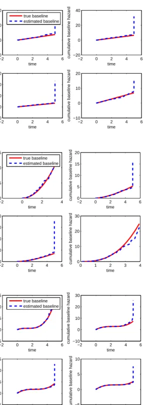
2.1.3 Estimation of the Cumulative Baseline Hazard . . . 26
2.2 Model Diagnosis . . . 28
2.3 Simulation Study . . . 29
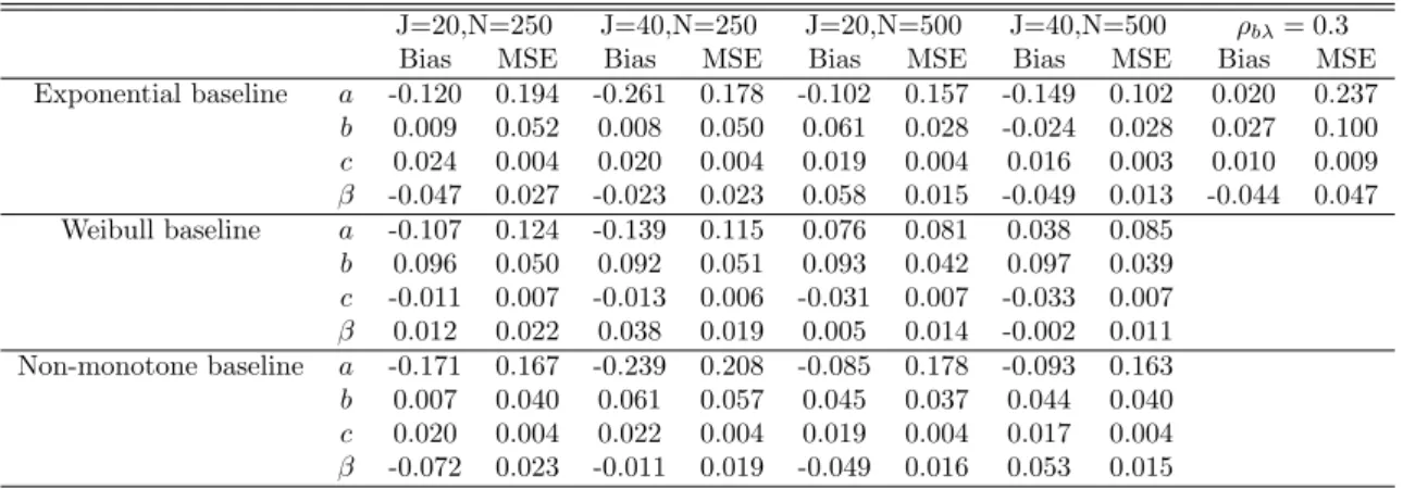
2.3.1 Study One: Check the Estimation Accuracy . . . 29
2.3.2 Results . . . 30
2.3.3 Study Two: When the Item Parameters are Correlated . . . 32
Chapter 3 The Linear Transformation Model with Frailties . . . 34
3.1 The Linear Transformation Model . . . 35
3.1.1 Hierarchical Linear Transformation IRT Model . . . 37
3.2 Model Estimation . . . 39
3.2.1 Rank-based Marginal Likelihood forβ . . . 40
3.2.2 Estimating Equation Method for ˆH(t) . . . 42
3.2.3 Parameter Estimation . . . 43
3.3 Model Diagnosis . . . 46
3.4 Simulation Study . . . 47
Chapter 4 Real Data Analysis . . . 52
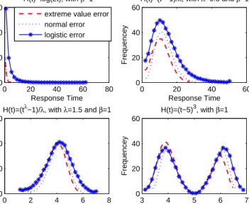
4.1 Marginal Distribution of Response Time . . . 52
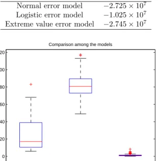
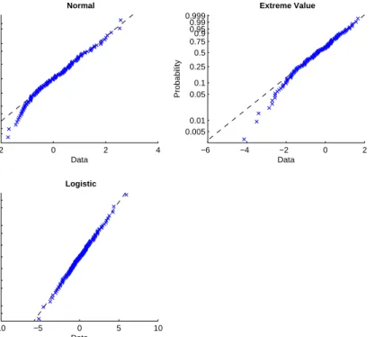
4.2 Model Selection . . . 54
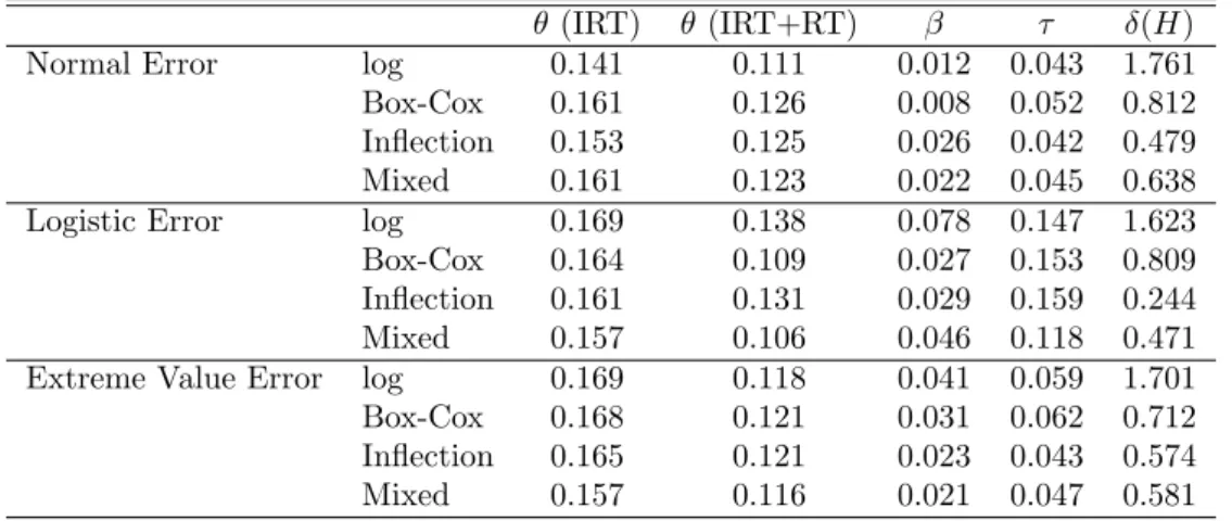
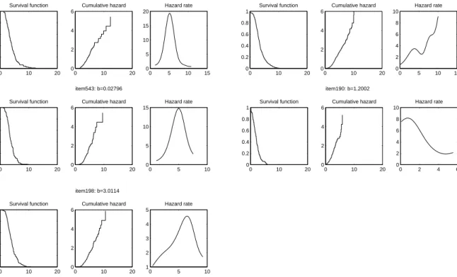
4.2.1 Linear Transformation Models with Different Error Distributions . . . 54
4.2.2 Parametric vs. Semi-parametric Models . . . 56
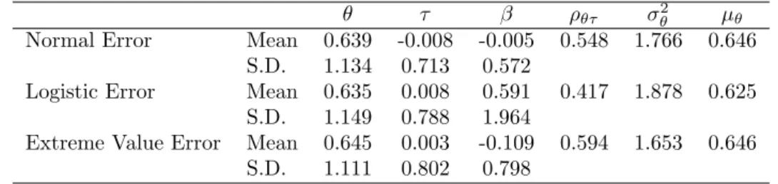
4.3 Parameter Estimation . . . 60
4.3.1 Fitting Cumulative Baseline Hazard with B-splines and Parametric Functions . . . 63
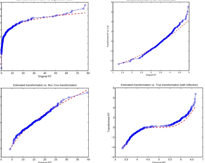
4.3.2 Recovering the Response Time Distribution: Survival Curves . . . 65
4.4 Further Model Diagnosis . . . 66
4.4.1 Local Independence Assumption . . . 66
Chapter 5 Alternative Methods of Semi-Parametric Model Estimation . . . 72
5.1 Modeling Non-Parametric Transformation Through Incomplete Beta Function . . . 72
5.2 Likelihood-Free Algorithm . . . 74
5.2.1 Likelihood-free MCMC Samplers . . . 75
Chapter 6 Discussion and Future Work . . . 77
6.1 Semi-parametric Modeling Approach . . . 77
6.2 Application of Response Time . . . 80
6.2.1 Redesign of Item Selection Algorithm in CAT . . . 80
6.2.2 Introduce Additional Covariates in the Model . . . 82
6.2.3 Constructing RT Models for Cognitive Psychology . . . 82
6.3 Summary . . . 83
Chapter 1
Introduction
Web-based assessment (i.e., on-line testing) is becoming a mainstream form of modern testing due to the internet’s flexibility, accessibility, and potential capacities for faster data analysis and reporting. It also makes the collection of examinees’ response times straightforward. The analysis of response times (RTs) on tests has recently attracted increase interest. A number of publications have demonstrated the utility of considering RTs on tests. In the realm of personality scales, RTs have been used to measure attitude strength (Bassili, 1996) or detect social desirability (Holden and Kroner, 1992). They have also been used as an additional predictor to enhance criterion validity (Siem, 1996). In the field of achievement tests, RTs have been used to evaluate the speededness of the test, to detect cheating behaviors, and to design a better test (e.g., van der Linden and Guo, 2008; van der Linden, 2009; Bridgeman and Cline, 2004). However, in order to use the full diagnostic potential of RTs, psychometric models are needed to analyze the relationship between the observed RTs and the test takers’ latent traits. There are at least three advantages of developing such latent trait models: (1) the latent traits underlying the RTs can be used in addition to latent ability underlying the response accuracy as predictors of future performance, thereby enhancing criterion validity (Siem, 1996); (2) the estimation of ability can be improved by jointly modeling RTs and response accuracy; (3) such models can be used in cognitive psychology for more rigorous cognitive theory development (Rouder, Sun, Speckman, Lu, & Zhou, 2003; Klein Entink, Kuhn, & Fox, 2009b).
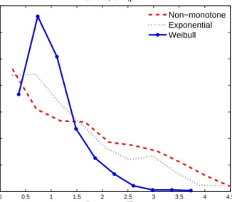
In the past couple of decades, researchers tried to formulate models that can maximally explain the variance of RTs as well as the connections among RTs, item characteristics and examinees’ behaviors. Most of the models are motivated by the “curve-fitting principle” in the sense that the proposed models are parametric representations of the underlying RT distributions (e.g., Ronder et al., 2003; Schnipke and Scrams, 1997; Klein Entink, van der Linden, & Fox, 2009). The models differ in terms of the assumed response time distributions (e.g., lognormal, exponential, Weibull, and etc), the underlying relations between ability and response speed, and the nature of the items for which the model is designed (Schnipke and Scrams, 2002). Although the parametric models have the advantage of conciseness, they may suffer from a reduced flexibility to fit real data. In addition, with an empirical data set, one often needs to fit each parametric model
separately until a best fitting model is decided based upon some model diagnostic criterion (Schnipke and Scrams, 1997). Even though, the best fitting model may not be the best one for each individual item in the item bank. Ranger and Kuhn (2012) demonstrated that the response time distribution differed dramatically across items within one test. This calls for a flexible model that relaxes the such distributional assumptions. The idea of proposing a “generalized model” that includes various parametric models as sub-models was first put forward by Ying and Chang (2005), and one example is the Box-Cox normal model (Klein Entink, van der Linden and Fox, 2009), where a power parameter was introduced to represent a number of different transformations. Most recently, Ranger and Kuhn (2012) proposed a generalized linear model with a flexible link function to model discrete response times. Specifically, their model includes a certain parameter (either at item level or test level) that determines the form of the link function, and their model unifies both proportional hazard models and accelerated lognormal failure time models. By fitting the generalized model to a data set, one can immediately pinpoint the most appropriate parametric form for each item from the estimation results.
This dissertation proposes another general modeling approach, namely, the semiparametric approach that reconciles the flexibility of nonparametric modeling and the brevity of the parametric modeling. Two semiparametric models are developed, one originates from the Cox proportional hazard model, and the other is built upon the linear transformation model. This latter model only assumes the existence of a monotone, but otherwise arbitrary transformation of the response times such that the linear model holds. As we will show, it includes the lognormal model, Box-Cox normal model, proportional hazard model and many other models.
Because the response time modeling has a long-term history, much wisdom has been accumulated. Also because this dissertation is motivated by the cutting-edge development in survival analysis, as a prelude for the next two chapters, brief introductions to both the current RT models and the survival analysis techniques are presented below.
1.1
Current Models for Response Time
Response time has been a preferred dependent variable in cognitive psychology since the mid-1950s (Luce, 1986). For relatively uncomplicated cognitive tasks such as Posner’s perceptual matching task (Posner and Boies, 1972), response times naturally indicate the processing procedures required by an individual to complete a task. The main idea being that the more (cognitive) steps or processes required to complete a task, the longer the response or reaction time. In testing, Gulliksen (1950) first coined the distinction
between power tests and speed tests. In a pure speed test, the items are easy and the examinees are asked to answer as many items as possible within a limited time period. The goal is to measure how quickly the examinees answer those items. In this sense, the speed test is similar to the simple cognitive tasks. In the pure power test, on the other hand, the items differ in difficulty and there are no time limits. For these tests, examinees’ response accuracies are of interest. In practice, although most of the tests (especially achievement tests) are power test, they also contain a speed component in that they are administered with a certain time limit.
Klein Entink et al. (2009a) summarized three different approaches that have been taken in the past to model RT. Here we briefly review each approach with representative examples. Under the first approach, only RT is modeled (Scheiblechner, 1979) such that it is mainly applicable to speed tests that have strict time limits. Within this category, Rouder et al.(2003) proposed a model based on Weibull distribution. In their model, the response time (also calledreaction time in cognitive psychology) tnj for personn on item j has the density
f(tnj) = πn(tnj−ψn) πn−1 σπn n exp ½ − · tnj−ψn σn ¸πn¾ , tnj > ψn, (1.1) whereψn,σnandπnare the shift, scale and shape parameters, respectively. Without incorporating any item level parameters, the model in (1.1) treats the RT for a given person as identically distributed across items, that is, characteristics of items do not impact RTs. This assumption is reasonable for the experimental paradigm (Rouder et al., 2003) where every stimuli in each trial requires almost the same cognitive process. The assumption might also hold when analyzing the “addition test” given to the second graders. Because in that test, the test takers can add single digit numbers (say, 100 of them) in 2 or 3 minutes, and every item has quite similar difficulty. When items differ in a test, Scheiblechner (1979) suggested exponential distribution of RT for personnresponding to itemj with density
f(tnj) = (τn+γj) exp[−(τn+γj)tnj]. (1.2)
In this model,τn is the person speed parameter,γj is the item speed parameter. Similar to the linear-logistic test model (LLTM; Fischer, 1973),γj can be further decomposed into fine-grained component process as
γj = K X k=1
ajkηk, (1.3)
where ηk indicates the time intensity of component process k, and ajk is the weight with respect to com-ponentk within itemj. Maris (1993) proposed using a more general gamma distribution but with similar
parameterizations as in (1.2). Although these well-established models are not explicitly characterized in the survival analysis framework, notice that Weibull, exponential and gamma distributions are all common parametric survival time distributions.
The second approach focuses on separate analysis of RTs and response accuracy. For instance, Gorin (2005) regressed log-transformed RTs on decomposed item difficulty parameter. Similar ideas are seen in Embreston (1998) and Primi (2001). Mulholland, Pellegrino, and Glaser (1980), on the other hand, used analysis of variance to predict RTs by item characteristics. Schnipke and Scrams (1997) proposed a lognormal model with a linear composition of its mean parameter into a general-level, person, and item component. That is, the logarithm of the time ofnthexaminee answer to thejthitem is decomposed as
logTnj =µ+δj+τn+εnj, (1.4)
where µ is the grand mean response-time for the item bank and the examinee population, τn reflects the speed of examinee n, δj reflects the time intensity of item j, and εnj ∼ N(0, σ2). The same model was used to control differential speededness (van der Linden et al., 1999) and to detect the examinees’ aberrant behaviors (van der Linden and van Krimpen-Stoop, 2003). In this approach, RTs and responses are modeled separately assuming these two variables vary independently. However, this assumption may not hold and thus a third approach was proposed.
The third approach advocates joint modeling of both RTs and responses, and such models include those proposed by Thissen (1983), van der Linden (1999), Roskam (1997), Wang and Hanson (2005), just to name a few. A major group of models in this category is motivated by the idea of a speed-accuracy relationship. Cognitive psychologist often focused on the within-person relationship, i.e., whether a person’s response accuracy will decrease if he or she chooses to perform a task more quickly? This is termed as “speed-accuracy” tradeoff. The psychometricians, however, are more interested in the across-person relationship between speed and accuracy. For example, one question that psychometricians often explore is whether examinees with higher ability tend to answer the items faster. Both types of speed-accuracy relationships are considered within the model suggested by Verhelst, Verstralen, and Jansen (1997), or Thissen (1983). In their models, the speed-accuracy tradeoff is reflected by letting response accuracy dependent on the time devoted to the item—spending more time on an item increases the probability of a correct response. The speed-accuracy correlation across examinees is reflected by the separate parameters of examinees’ ability (or mental power) and speed. Specifically, Verhelst et al.(1997) modeled the probability of a correct response
on itemj by examineenas
Pj(θn, τn) = [1 + exp(θn−lnτn−bj)−πj], (1.5) where bj is the difficulty parameter for itemj, θn and τn are the ability and speed parameter for the nth person, and πj is an item-dependent shape parameter. For π = 1, the model reduces to a Rasch type model withξn =θn−lnτn replacing the traditional ability parameter. The speed-accuracy tradeoff is just reflected through ξn. That is, if a person decides to increase the speed τn, ξn will decrease and so does the correct response probability. Roskam (1997) proposed a similar model that is a Rasch model with an additive parameter structure incorporating logarithm of time as a regressor
Pj(θn) = [1 + exp(θn+ lntnj−bj)−1]. (1.6)
The model assumes a speed-accuracy tradeoff directly between the ability of the test taker and the actual time spent on a test item; less time on an item results in a higher speed and lower accuracy. Model (1.6) assumes that the actual RT is equivalent to examinees’ speed. Though this assumption may be reasonable in the experiment paradigm, it may not hold in testing, in particular when each person takes a different set of items as in adaptive testing. Therefore, it is necessary to make a distinction between the RTs on the items and the speed at which the examinees’ operate throughout the test. In this sense, a better way to measure speed is through distinct parameterizations of examinees’ speed and items’ time intensity. Such a modeling idea is reflected in Thissen (1983)’s model that takes the following form:
lnTnj =µ+τn+βj−ρ(ajθn−bj) +²nj, (1.7)
where²nj ∼N(0, σ2). The normally distributed error term indicates that the model belongs to the lognormal family. Parametersτnandβjcan be interpreted as the speed of the examinee and the amount of time required by the item. The parameterµis a general intercept parameter, aj,bj, andθn are the item discrimination, item difficulty and examinee ability parameters respectively. The termρ(ajθn−bj) represents a regression of a two-parameter response model on the logarithm of time withρbeing the regression parameter. The speed accuracy tradeoff is indicated by the termρ(ajθn−bj) whenρ <0. Whenρ >0, the speed accuracy relation reverses. A similar idea was adopted by Ferrando and Lorenzo-Seva (2007) in modeling response time data from binary personality items, and the only change is the regression term. Instead of using (ajθn−bj), they used a distance measureδij=
q
a2
j(θi−bj)2 based on a distance-difficulty hypothesis in personality theory. Van der Linden (2007) argued that although the speed-accuracy tradeoff is prevalent in reaction-time
research, on a test with a reasonable time limit, there is no need to incorporate a tradeoff in a RT model for a fixed person and a fixed set of test items (van der Linden, 2007). In other words, the tradeoff is a within-person constraint only, and it does not provide information to predict the speed or accuracy of one person from another. Therefore, the speed at which the test taker operates on the items should be assumed as a latent trait, and the response accuracy should only be determined by the examinees’ abilities. In fact, as early as 1930, Kennedy (1930) found that individuals tended to perform at a consistent rate of work across a variety of cognitive tasks, even after partialing out the intelligence difference (Schnipke and Scrams, 2002). This conclusion is supported by Tate (1948), who investigated the speed accuracy relationship on number series, arithmetic reasoning, and spatial relations questions. He found that when accuracy was controlled, the fastest examinees were not the most accurate but fast subjects were consistently fast and slow subjects were consistently slow. These results illuminate that we need to model accuracy exclusively dependent on ability, and response time exclusively dependent on examinees’ latent speeds. But on the second level of the model, the speed and ability can be correlated. The correlation may differ depending upon the test context and content (Schnipke and Scrams, 2002).
Following this argument, van der Linden (2007) proposed a hierarchical framework, in which RT and responses are modeled separately at the measurement model level; and at a higher level, a population model for the person parameters (speed and ability) is constructed to account for the correlation between them. This model distinguishes the speed-accuracy tradeoff within a person from the speed-accuracy correlation in the population. The formulation of the model is as follows. At the first level, two models for the responses and RTs are specified separately. Responses are assumed to follow a three-parameter logistic (3PL) model:
Pj(θn) =cj+ (1−cj) exp[aj(θn−bj)]
1 + exp[aj(θn−bj)], (1.8) where aj, bj, and cj represent item discrimination, difficulty and guessing parameters. For the RTs, a lognormal model with separate person and item parameters was adopted (van der Linden, 2006),
Tnj ∼f(tnj;τn, αj, βj)≡ αj tnj √ 2πexp ½ −1 2[αj(lntnj−(βj−τn))] 2 ¾ , (1.9)
where τn, βj and αj are the speed parameter for examineen, the time intensity and discriminating power of itemj, respectively. At the second level, ξn= (θn, τn) is assumed to be randomly drawn from a bivariate normal distribution, with mean vector µp = (µθ, µτ), and covariance matrix Σp =
σ 2 θ σθτ σθτ στ2 . Anal-ogously, the item parameter vectorψj = (aj, bj, cj, αj, βj) is also assumed to follow a multivariate normal
distribution with mean vectorµJ= (µa, µb, µc, µα, µβ)0, and covariance matrix ΣJ = σ2 a σab σac σaα σaβ σba σb2 σbc σbα σbβ σca σcb σ2c σcα σcβ σaα σαb σαc σα2 σαβ σβa σβb σβc σβα σ2β .
Several recent attempts have been made to extend the above hierarchical model for more complicated applications. For example, instead of only considering log transformation of RT, Klein Entink, van der Linden and Fox (2009) considered a broader class of Box-Cox transformations (Box and Cox, 1964). This generalization leads to a normal model for the transformed RTs,
T(v)= tv nj−1 v ∼N(βj−τn, α −2 j ) v6= 0 logtnj ∼N(βj−τn, α−j2) v= 0
Here T denotes the original time andT(v) denotes the Box-Cox transformed time. It is apparent that the lognormal distribution belongs to the Box-Cox transformation. Further, Klein Entink, Fox and van der Linden (2009) proposed a multivariate multilevel model for mixed response variables (binary responses and continuous RTs). Their model allows for the incorporation of explanatory variables to identify factors that explain variation in speed and accuracy between individuals who may be nested within groups. Another attempt was made by Klein Entink, Kuhn, Hornke and Fox (2009). They proposed a joint modeling approach by use of responses and RTs to evaluate cognitive theory. Their model takes a similar structure as van der Linden’s (2007) hierarchical model, and the innovation is to decompose each item parameter based on the detailed cognitive process as required by the item in order to support the cognitive theory that underlies the item design (Klein Entink et al., 2009b).
1.2
Mixed (Multilevel) and Conditional Regression Perspective
The construction and evolution of response time and response accuracy modeling can also be summarized from mixed and conditional regression perspectives. When analyzing the experimental data from cognitive psychology, there is much literature on the speed-accuracy tradeoff (Kahane and Loftus, 1999) and on mathematical processing models for response speed and accuracy (Luce, 1986; Ratcliff, 1988). These models, however, do not distinguish between person and item parameters, and they are only applicable to
within-subject analysis of a series of replications of the same stimuli in a psychophysical discrimination or detection task (van Breukelen, 2005). On the contrary, in testing or in cognitive tests that typically include tasks like analogical reasoning or series completion, the items vary by difficulty and there is only one replication per person per item. A better approach for this application is, therefore, an extension of item response theory models into the simultaneous modeling of both speed and accuracy as functions of the person and item parameters, such as the models that will be proposed in this dissertation.
The traditional IRT modeling and fixed effects logistic regression can be combined into what is known as mixed or conditional logistic regression. For instance, let the log-odds of a correct response by person i on itemj as log · pij (1−pij) ¸ =β0i+β1iX1ij+....+βpiXpij, (1.10) where pij is the correct response probability by person i on item j, and X1 to Xp represents observed covariates that could either be between-subject (person level) variables such as age or gender, or within-subject (item level) variables like the number of cognitive steps needed to solve an item, or interaction of both. If the covariate is the response time spent on the item, this model inherently models the speed-accuracy tradeoff. The parameterβ0i is person dependent intercept,β1i throughβpiare person dependent regression weights. The well-known Rasch model can be viewed as one special case of model (1.10) (van Breukelen, 2005).
Similarly, response time could also be modeled via linear mixed modeling approach (Verbeke and Molen-berghs, 2000). Because response times are frequently assumed as following a lognormal distribution within persons and items, the mixed model could be
log(tij) =γ0i+γ1iX1ij+...+γpiXpij+eij, (1.11)
where eij is normally distributed error term. As in (1.10), γ0i through γpi are person level intercept and slopes. The above two mixed regression models treated persons as random but items as fixed. However, as both subjects (persons) and items can be regarded as random samples from a population of people and a population of items, one can define random residuals for both subjects and items. When subjects and items are in a non-hierarchical relationship, such a model is referred to as a crossed random effect model (Raudenbush, 1993). For instance, Baayen, Davidson, and Bates (2008) proposed a mixed effects modeling approach with crossed random effects for subjects and items, their model can be expressed as
where Tij represents response time for subjecti on item j, τi ∼ N(0, σ2τ) and α1j ∼ N(0, σ2α1) denote the
random intercepts for subject (i.e., examinees’ latent speed) and item, respectively, where as X1i andX2j denote the fixed effects. In this model, there is no by-subject or by-item random slopes for simplicity. εij is the by-observation error term. Here the response time itself is modeled directly, but sometimes, certain transformation of response time, say, log transformation, could be imposed first. Following the similar argument, Jaeger (2008) proposed a similar model for response accuracy as
ln µ pij (1−pij) ¶ =β0+β1X1i+β2X2j+θi+α2j+εij, (1.13)
withθi∼ N(0, σ2θ) andα2j∼ N(0, σ2α2). Large values ofθcorrespond to higher participant error rate (i.e.,
lower ability) and large values ofα2 indicates the items have higher difficulty.
The estimation of response time and response accuracy models are separately discussed in Baayen et al. (2008) and Jaeger (2008). Loeys, Rosseel and Baten (2011) recently proposed a joint model by imposing a joint multivariate distribution on the vector of all random effects for subject and item, as follows
Σs= σ 2 τ ρθτσθστ ρθτσθστ σ2θ , and Σs= σ 2 α1 ρα1α2σα1σα2 ρα1α2σα1σα2 σ 2 α2 .
The parameterρθτ measures the correlation between speed and ability at subject level, whereasρα1α2
mea-sures the correlation between time intensity and difficulty at item level. This modeling approach resembles van der Linden (2007)’s hierarchical framework.
1.3
Survival Analysis and Educational Measurement
Survival analysis is a branch of statistics that concerns the analysis of time-to-event data. Some of the questions survival analysis try to tackle are: what is the proportion of a population that will survive beyond a particular time; among the survivors, at what hazard rate will they die or fail; what factors and how will the factors affect the survival probability or hazard rate of a population. The primary objective of interest is the survival function, specifying the probability that the occurrence (death) of an event is later than some particular time. Survival function is often defined as S(t) = P(T > t), where t is some time,
andT is a random variable denoting the time of death. The survival function must be non-increasing, i.e., S(t1)≤S(t2) ift1≤t2. This reflects the idea that survival to some later time requires survival at all earlier times as well.
Survival analysis has benefited medical scientists in the study of mortality due to chronic diseases, and has helped industrial statisticians to model the longevity of machinery and parts in manufacturing processes. In principle, survival analysis techniques could be used in any science in which outcomes are measured as the time until an awaited event (Douglas, Kosorok and Chewning, 1999). Psychology is also a specific area that survival analysis can shed light on. For instance, Douglas et al. (1999) proposed a discrete version of proportional hazard frailty model to explain the substance abuse of youths. In particular, they modeled the ages at which youths first try alcohol, cigarettes, marijuana, and inhalants, as a function of their latent psychological abilities to abstain from substance abuse. Another example is by Singer and Willett (1993) who used discrete-time survival analysis to study whether and, if so, when the public school teachers stopped teaching between their first year of teaching and the year when the data collection ended. The discrete-time hazard model proposed in their paper not only answers these descriptive questions but also models the relationship between event occurrence and predictors as well. The specific area in educational measurement that survival analysis come into play is response time analysis. Response time (RT) is the time period from the onset of an item until examinee provides an answer to the item. If viewing “giving a response” as an event, RT shares the same meaning as the survival time in biostatistics, and therefore RT can be modeled directly through the survival functionS(t).
The most common way to estimate S(t) is through the now ubiquitous Kaplan-Meier estimator (named after Edward L. Kaplan and Paul Meier), also known as the product-limit estimator. It is a non-parametric estimator derived from counting process. The specific construction of Kaplan-Meier estimator is as follows. For thejthitem, let the observed response time for theN examinees answering this item bet
1≤t2≤ · · · ≤ tN. Corresponding to eachti is the number of examinees ni whose RTs are longer than ti (“at risk” set) and the number of examineesdi who give response to itemj atti. The Kaplan-Meier maximum likelihood estimator ˆS(t) is a product ˆ S(t) = Y ti≤t (1−di ni ). (1.14) ˆ
S(t) is a non-decreasing step-function, with steps at ti,1 ≤i ≤N. The original Kaplan and Meier paper that appeared in 1958 is one of the most heavily cited papers in all of the sciences (Hubert & Wainer, unpublished). The importance of Kaplan-Meier curve is apparent in medical/pharmaceutical areas. In educational measurement, Kaplan-Meier curve also provides an overall description of the response time
distribution of an item. For example, Kaplan-Meier curve indicates on average what the probability equals that an examinee answers itemj within a time periodti. Oftentimes, harder items require longer time to answer, and therefore, the Kaplan-Meier curves of the difficult items are often flatter than those of easy items. Another advantage of the Kaplan-Meier estimator is that it has a closed form variance estimator (e.g., the Greenwood formula), and therefore the confidence band around the Kaplan-Meier curve is easily specified.
1.3.1
Regression Models
The Kaplan-Meier estimator only provides a marginal view of the RT distribution for an item, and it does not consider the item-person interaction, that is, the same item may have a different RT distribution for different examinees. To incorporate examinees’ parameters (that can be viewed as covariates) into the analysis of RT, we need to resort to regression models. In survival analysis, the covariates can enter into the model in a similar way as in common regression models. In the following, we will separately review two groups of regression models, parametric models and semi-parametric models.
The parametric models assume a fully parametric form of the survival function, or equivalently, the hazard function of response time. The hazard function (usually denoted ash(t)) is the instantaneous rate at which events occur. It is defined as
h(t) = lim δt→0
P[t≤T < t+δt|T ≥t]
δt .
In psychological terms, the hazard rate can be viewed as the processing capacity of an individual, the individual’s relative ability to perform mental work in a unit of time. Individuals with a high hazard rate (high conditional probability of finishing the task in the next moment) have a high processing capacity and work more intensely (Wenger & Gibson, 2004). The hazard rate relates to the survival function through S(t) = exp[−H(t)],where H(t) =Rs=0t h(s)dsis the cumulative hazard function. Taking exponential model
as an example, the hazard function at timet for an item with covariateZcan be written as
h(t|Z=z) =λc(z).
In this model, the hazard rate for a givenZ is a constant characterizing the exponential distribution. The covariate can be any observed or latent variables, such as the examinees’ demographic information, their latent ability, and the like. The function c(·) may be parameterized in a number of ways, oftentimes, the
effects of the covariates are reflected through a linear function,Z0β, and therefore
h(t|Z=z) =λc(z0β).
Hereβ0= (β
1, ..., βp) are regression parameters andcis a specified functional form. The choice ofcdepends on the particular data being considered, and three common forms have been used in the past (e.g., Feigl & Zelen, 1965): (1) c(Z) = 1 +Z, (2)c(Z) = (1 +Z)−1, and (3) c(Z) = exp(Z). The first two forms correspond to (1) the hazard rate and (2) mean survival time, being linear functions of Z. The last form that is also the most widely used form, assumes that a unit increase in a covariate is multiplicative with respect to the hazard rate.
Now consider the model with hazard function
h(t|Z=z) =λexp(z0β). (1.15)
Taking log transformation on both sides yield a model specifying that the log hazard rate is a linear function of the covariateZ. In terms of the log survival time,Y = logT, the above model can be reparameterized as
Y =α−Z0β+W, (1.16)
where α=−logλand W follows the extreme value distribution. The model in (1.16) can be viewed as a log-linear model, and it is a linear model forY with the error termW having an extreme value distribution. Another well-known parametric regression model is based on Weibull distribution, with the covariate entered into the model in essentially the same way. Specifically, the conditional hazard is expressed as
h(t|Z=z) =γλ(λt)γ−1exp(z0β). (1.17)
Due to the exponential link function (i.e., c(Z) = exp(Z)), the effect of the covariates is again acting multiplicatively on the Weibull hazard. By the same token, letY = logT, the model (1.17) can be expressed in the linear form as
Y =α+Z0β∗+σW, (1.18)
where α = −logλ, σ = γ−1 and β∗ = −σβ. The error term W again follows standard extreme value
distribution.
covariates in both models (1.15) and (1.17) act multiplicatively on the hazard function. This generalization, as will be shown below, suggests a typical semi-parametric model called therelative risk model orCox model. On the other hand, both of these models can be expressed in a log-linear form; that is, the covariates act additively on the log transformed timeY, and this general class of log-linear models is called theaccelerated failure time model.
In the above models, the covariates are assumed to be observed. Biostatisticians first recognized the usefulness of latent variables to model survival times that are correlated due to either repeated measurements taken on a single subject, or measurements of a common variable taken on genetically associated subjects. These needs gave rise to frailty models, in which a latentfrailty random variable is included in the model to account for possible correlations in failure time distributions (Clayton, 1991; Clayton and Cuzick, 1985). The frailty variables may be viewed as random effects and usually only the influence of the explanatory covariates on failure time is the primary concern. Douglas et al.(1999) used the frailty model in psychology, and their model is a similar version of the conditional proportional hazard model (Clayton and Cuzick, 1985), in which the hazard function for each failure time is a product of the baseline hazard, frailty random variable, and covariate effects. The unique feature of their model is that it has an item-level parameter that measures the influence of the latent variable on the failure time. Thus separate items differ with respect to the extent that the latent variable influences responses. In fact, the Cox PH model represents a standard approach in survival time analysis, it makes only very mild distributional assumptions and, is a flexible semiparametric model. However, it is only very recently that the Cox model has been introduced in the filed of measurement to analyze response times (Ranger and Ortner, 2011). In Chapter 2 of this dissertation, we propose to use Cox model for RT analysis, and that chapter is complementary to Ranger and Ortner’s earlier research.
A third widely used parametric regression model comes from log-normal distribution of time (van Breuke-len, 2005; van der Linden, 2007). The lognormal regression model takes the following form in general
log(t|Z=z) =z0β+ε,
whereε∼ N(0, σ2). Then the hazard function can be written as
h(t) = 1 tσφ ¡logt−z0β σ ¢ Φ¡−logσt+z0β¢,
where φ(·) and Φ(·) are the probability density function and cumulative density function of the standard normal distribution, respectively. Apparently, the covariate is not multiplicatively related to the hazard
function, and the effect of the covariates cannot be written in an exponential link function as in exponential or Weibull regression models. Because of these reasons, the lognormal regression model is not a special case of the proportional hazard model. However, it does belong to thelinear transformation model family, and this drives the development of the second new model in the dissertation. In Chapter 3, we will review the linear transformation model, and show how it subsumes both Cox model and lognormal model as special cases.
A semi-parametric extension of the above parametric models with exponential link function leads to theCox proportional hazard model. The Cox model combines the parametric regression term with a non-parametrically defined baseline hazard function. Therefore, the hazard function of the Cox model is expressed as (Cox, 1972)
h(t|θ) =h0(t) exp(z0β).
Here the non-parametric baseline hazardh0(t) reflects the flexibility of the model to accommodate a variety of different shapes of RT distributions, whereas the regression term succinctly summarizes how RT changes with the covariates. When the baseline hazard is a constant, this model becomes the exponential regression model; when the baseline hazard takes the form ofh0(t) =γ(λt)γ−1, the model becomes Weibull regression model. In light of this, the Cox model is flexible enough to represent different RT distributions, and thus it serves as a good candidate for modeling RTs. The new model proposed in Chapter 2 derives from the Cox model with a frailty term, and the frailty represents the examinee’s latent speed.
1.3.2
Model Diagnostic Techniques
Model fit and adequacy checking play an important role in survival analysis. In the classical survival analysis framework, an assessment of the hazard function is usually done through so-calledhazard plot. Specifically, a parametric specification for the hazard,h(t), can be checked using an empirical estimate ofh(t), say, ˆh(t). Plots of ˆh(t) versust(or log(t)) are compared with plots assuming the parametric model. Another approach is based on residual analysis, in which a theoretical or empirical Q-Q plot (see, e.g., Cox and Oakes, 1984; Therneau et al., 1990) is developed for certain exponential or martingale based residuals. In this section, we will introduce the second approach in detail for the Cox model under both frequentist and Bayesian paradigms.
In frequentist paradigm, the Cox-Snell (1968) residual can be used to assess the overall fit of model. For item j, denote the observations as (Ti, δi,Zi), i = 1,2, ..., n. For simplicity, we assume Zis are time independent; and also due to the fact that all RTs in tests are observed, we drop the censoring indicatorδiin the following. Suppose the proportional hazard modelh(t|Zi) =h0(t) exp(Z0iβj) has been fit to the model. If
the model is correct, then the true cumulative hazard function conditional on Z,H(T|Z), has an exponential distribution with hazard rate equal to 1. This conclusion holds becauseH(T|Z) =−ln[1−F(T|Z)] where F(T|Z) is the cumulative distribution function and it follows uniform distribution. So the cumulative distribution function ofH(T|Z) is 1−exp(−H) that is exactly the c.d.f of the unit exponential distribution. Now, let ˆβdenote the maximum likelihood (it is actually the partial likelihood that will be introduced in Chapter 2) estimate ofβ, and let ˆH0denotes the estimator of the baseline hazard rate. Then the Cox-Snell residual for theith examinee andjth item is defined as
rij = ˆH0(ti) exp(Z0iβˆj). (1.19)
It is easy to notice thatrij will be approximately exponentially distributed with hazard rate 1, given that the proportional hazards model is correct and ˆH0 is close to H0 and ˆβ is close to β. To check whether therijs behaves as a sample from a unit exponential, the Nelson-Aalen estimator of the cumulative hazard rate of the rij, i = 1, ..., n can be computed for each item separately. If rijs are from a unit exponential distribution, then this estimator should be approximately equal to the cumulative hazard rate of the unit exponential HE(t) = t. Thus, a plot of the estimated cumulative hazard rate of theri, ˆHr(rij), versusrij should be a straight line through the origin with a slope of 1.
Here we only review the Cox-Snell residual for the simplest case where the covariates do not depend on time. This assumption is reasonable in response time research where the covariates often include examinees’ abilities, speed, or other demographic variables such as age, social economic status, etc. Assuming fixed ability and fixed speed for a person during the test, stationarity assumptions leads to standard item response modeling (van der Linden 2007). However, if time-dependent effects such as fatigue or practice are modeled, more complex models need to be constructed and the Cox-Snell residual can be modified accordingly.
For the parametric regression model, the Cox-Snell residual is redefined to incorporate the specific para-metric form of the baseline hazard rate. For example, the Cox-Snell residuals for the exponential and Weibull regression models areri= ˆλtiexp(Z0iβˆj) andri= ˆλexp(Z0iβˆj)tαiˆ, respectively. In fact, examination of model fit with the Cox-Snell residual is equivalent to that done using the standardized residual based on the log-linear model representation. To be specific, we define the standardized residual by analogy with those used in normal regression theory as
ri= logTi−αˆ−Zˆ 0 iβj ˆ σ . (1.20)
Chapter 2
The Hierarchical Proportional Hazard
Model
This chapter introduces a new hierarchical proportional hazard model to model RTs and response accuracy simultaneously. A critical feature of the model is that examinees’ abilities are distinguished from their latent speed and separate latent traits are assigned to both of them. This leads to the key assumption of the current model: a test taker operates at a fixed level of speed during the course of the tests. This stationarity assumption excludes changes in behavior during the test due to fatigue, learning, strategy shifts and other factors. The hierarchical framework proposed by van der Linden (2007) is adopted here. Measurement models at the first level separate the variability in the observed responses and RTs into item and person effects. At a higher level, we assume the examinee’s abilityθand latent speedτare from a bivariate normal distribution. The specific formulation of the model is as follows.
First-Level Model. At the first level, two models for the responses and RTs are specified separately. For the item response model, any appropriate parametric model may be used, but we focus on the three-parameter logistic model:
Pj(θi) =cj+ (1−cj) exp[aj(θi−bj)]
1 + exp[aj(θi−bj)], (2.1) with aj, bj, and cj representing item discrimination, difficulty and guessing parameters. For the response times, the Cox PH model is chosen and the hazard function for RTs is
hij(t|τi) =h0j(t) exp(βjτi) (2.2)
where the survival function is
p(tij ≥t|τi) =Sij(t) = exp · − Z t 0 h0j(s) exp(βjτi)ds ¸ , (2.3)
whereτi∈ Ris the speed parameter for test taker i. The subscriptj inh0j implies that different shapes of the RT distributions are possible for different items, andβj is the regression parameter (i.e., slope). When βj is positive, the higher theτi, the shorter the RT will tend to be. Whenβj is negative, it means examinees
with higher answering speed tend to take a longer time to finish the item. This measurement model resembles the one proposed by Ranger and Ortner (2011). Theβj coefficient also determines the influence of the latent speed on the hazard rate. In a psychological sense, it controls the increase in processing capacity that is due to a unit increase in the latent speed. Notice that in traditional survival analysis, the regression parameter is interpreted in a relative sense. But in educational measurement, it is important to be able to make inference about examinees and items, such as how much time is required for each examinee on a particular item on average. Therefore, both the regression parameter and baseline hazard have to be estimated accurately. This point is re-emphasized in the model estimation section below. As every constant multiplier can be absorbed in the baseline hazard rate, the linear predictorβjτidoes not include an intercept term. The item time intensity is reflected in the baseline hazard, and more clearly via equation (2.3). In general, items with lower cumulative hazardH0(t) tend to be more time consuming.
Second-Level Model. This part of the model captures the joint distribution of the person parameters in a population. The values of ξi = (θi, τi)0 are assumed to be randomly drawn from a bivariate normal distribution, i.e., ξi∼f(ξi;µp,Σp)≡ |Σ−p1|1/2 2π exp · −1 2(ξi−µp) TΣ−1 p (ξi−µp) ¸ , (2.4)
with mean vector
µp= (µθ, µτ), and covariance matrix
Σp= σ 2 θ σθτ σθτ σ2τ .
Identifiability. To establish identifiability, we suggest the constraints µθ= 0, σθ2= 1, µτ = 0, στ2 = 1. Here, the first two constraints are standard in IRT parameter estimation, when item parameters are unknown. The last two constraints fix the scale ofτ to remove the tradeoff between βj and τi and they also fix the scale ofh0.
Model Assumption. Following van der Linden (2007), this model has three independence assumptions. They are
• Independence between responses givenθ, that is
f(yi1,· · ·, yiJ|θi) = J Y j=1
• Independence between response times givenτ . This assumption is defined as f(ti1,· · ·, tiJ|τi) = J Y j=1 f(tij|τi), (2.6)
• Independence between responses and response times given θandτ. That is
f(ui1,· · ·, yiJ;ti1,· · · , tiJ|θi, τi) = J Y j=1
f(yij|θi)f(tij|τi) (2.7)
In van der Linden (2007)’s model, he imposed a covariance structure on item parameters, whereas we assume the item parameters are independent of one another. There are three reasons. First, according to the results in van der Linden (2007), only the correlation between item time intensity and item difficulty is non-zero (with posterior mean 0.3), all the rest correlations are either very close to 0 or have posterior confidence interval covering 0. Second, the item time intensity information in the new model is reflected in the non-parametric baseline hazardh0j(t), whose correlation with the item difficultybjis not easily modeled. Only when the parametric form ofh0j(t) is known, for instance, in exponential model,h0j(t) =λj, that one can model the correlation between λand b. In this case, because Sij(t) = exp[−exp(βjτi)(λjt)], λand b should be negatively correlated, indicating that more difficult times are more likely to be time consuming. Third, as shown in our simulation study below, even when the correlation between item time intensity and item difficulty is ignored, the estimation accuracy will not be significantly affected.
2.1
Model Estimation
The goal of our investigation is to accurately estimate θ and τ, as well as the regression parameter β in response time model of (2.3) and item parameters in (2.1). In many Cox frailty model applications, only the regression parameterβ and frailtyτ need to be estimated, but in our case, in order to make inference about the examinees and items, the non-parametric cumulative baseline hazard H0 also needs to be estimated. Several approaches were proposed in the past to estimate both parametric and non-parametric parts of the Cox model, such as estimation based on a spline approximation of the baseline hazard rate (Cai, Hyndman, & Wand, 2002) or estimation based on piecewise exponential models (Friedman, 1982). Two approaches that have advantages (Ranger and Ortner 2011) are (1) estimation by treating response time as discrete variable (McCullagh, 1980), such that the Cox model can be viewed within the generalized linear model framework and standard software can be used for model estimation; (2) estimation based on partial likelihood;
this approach does require categorization of the response times and thus it is more efficient (Ranger and Ortner 2011). Ranger and Ortner (2011) explored both methods, and they employed a divide-and-conquer approach by estimating the parametric part first and non-parametric part secondly. We proposed a two-stage estimation method that shares the same principle, but instead of using partial likelihood within the marginalized maximum likelihood framework, we used it within the Markov chain Monte Carlo (MCMC) framework.
Marginal likelihood inference involving latent variables is usually challenging because of the integrals that are sometimes numerically intractable. One approach that avoids such difficulties is to use the MCMC method to obtain draws from a distribution that has a density proportional to the joint posterior distribution of the item and person parameters. Another motivation for using the MCMC method is that in computerized adaptive testing (CAT), every test taker is given different items, based on his or her adaptively estimated θ level. So the random sampling ofθ (orτ due to the possible correlation between them) from a common distribution can not be assumed. We wish for our estimation technique to allow for data obtained by CAT. Consequently, the usual marginal likelihood approaches used in latent variable modeling are no longer appropriate.
Estimating Cox’s PH frailty model with MCMC is not entirely new. Clayton (1991) used Gibbs sampling to fit frailty models to clustered failure data. He sampled iteratively from the full conditional distribution ofH0j and all parameters withH0j as an independent increment gamma process (Kalbfleisch, 1978). Gray (1994) used a piecewise constant baseline hazard and also included it as a parameter to be updated in the MCMC scheme. Similarly, Douglas et al.(1999) modeled the discrete failure time, and treated the baseline hazard as a constant at each time point, which again was incorporated in the MCMC algorithm. Most recently, Henschel, Engel, Holzel, and Mansmann (2009) treated the baseline hazard with a stepwise constant function as well as a cubic spline. Sharef, Strawderman, Ruppert, Cowen, and Halasyamani (2010) argued that treating baseline hazard as piecewise constant is somewhat too restrictive because it depends on some discretization of time. Instead, they proposed to model the baseline hazard as a penalized mixture of B-splines. Their approach is even more general in that they allowed the frailty distribution to be unspecified, and modeled it as a penalized mixture of normalized B-splines. As a result, their model estimation method continues to apply to the proportional hazard frailty model, while permits shrinkage towards a specific parametric hazard function or frailty distribution.
Although the Sharef et al. (2010)’s method is flexible and promising, it does not lend itself directly to our case because of two reasons: (1) in our model, we assign an item level regression coefficient βj in front of the frailty termτi whereas in their model, the effect of the frailty is the same across different items; (2) in
our model, we impose a covariance structure on the frailty term, which introduces extra difficulty in model estimation. Due to these reasons, we propose a two-stage estimation method. In the first stage, we avoid the difficulty of modeling and sampling fromH0j by using the Cox partial likelihood (Cox, 1975), and in the second stage, we estimate the infinite-dimensional parameterH0j through either non-parametric estimator or B-splines. The use of partial likelihood in the Bayesian context for the frailty model estimation has been demonstrated in Gustafson (1997) and Sargent (1998). The justification for using partial likelihood will be briefly described in section 2.1.2.
2.1.1
Partial Likelihood
For thejth item, suppose that there are no ties between the response times. Lett(1j)< t(2j)<· · ·< t(N j) denote the ordered RTs andτibe the latent trait associated with the individual whose response time ist(ij). Define the risk setR(t(pj)) at time t(pj), 1≤p≤N, as the set of all individuals who have not answered the question yet, i.e.,R(t(pj)) ={t((p+1)j),· · ·, t(N j)}. The partial likelihood function for thejth item given τ is specified as: L(βj|τ) = N Y i=1 exp[βjτi] P tpj∈R(tpj)exp[βjτp] = N Y i=1 exp[βjτi] PN p≥iexp[βjτp] (2.8)
The partial likelihood for the vectorβ= (β1,· · · , βJ)0 is then defined as
L(β|τ) = J Y j=1
L(βj|τ). (2.9)
The log of the partial likelihood isLL(βj|τ) = ln[L(βj|τ)], and we writeLL(βj|τ) as
LL(βj|τ) = N X i=1 βjτ(i)− N X i=1 ln[ N X p≥i exp(βjτp)]. (2.10)
Taking derivatives with respect toβ we find the score,U(βj|τ) =∂LL(βj|τ)/∂βj, equals to
U(βj|τ) = N X i=1 · τ(i)− PN p≥iτ(p)exp[βjτp] PN p≥iexp[βjτp] ¸ . (2.11)
Kalbfleisch and Prentice (1973) demonstrated that the partial likelihood is a marginal likelihood forβ arising out of the distribution of the rank vector associated with the failure times (or response times). The use of
the partial likelihood for inference onβ has been justified from both the frequentist viewpoint (Anderson and Gill, 1982) and the Bayesian viewpoint (Kalbfleisch, 1978).
2.1.2
Parameter Estimation: Markov chain Monte Carlo
Suppose the items are indexed by j= 1,· · · , J,and the examinees byi= 1,· · · , N. For the ith test taker, his or her responses and response times are denoted by Yi = (Yi1,· · · , YiJ)0, and Ti = (Ti1,· · · , TiJ)0, respectively. We model the jth item’s hazard function by (2.2) and specify the partial likelihood function by (2.8). We assume a three-parameter IRT model (2.1) for the response variable Yi, then the likelihood function for theith subject’s abilityθi can be specified as
IRT(θi) = J Y j=1
Pj(θi)yij(1−Pj(θi))1−yij. (2.12)
To estimate the parametersβ= (β1,· · ·, βJ)0, note that in CAT it would generally be the case that different examinees take different items, and the items they take are closely associated with their ability levelθ(so is related withτ as well). This means some off-the-shelf methods for marginal likelihood estimation or a frailty model procedure will not work. So in our investigation, a Bayesian MCMC method (Metropolis-Hastings algorithm) is used instead. The MCMC method generates samples fromπ(ω) by creating a Markov chain on the state space ofω that has its equilibrium distribution π(ω). Theoretical details on MCMC methods can be found in Tierney (1994).
Our objective is utilizing the RT information to estimate the non-parametric baseline hazardh0, regres-sion parameterβ, item parametersa, b, c, examinees’ speed parameterτ, and also obtain more information for the estimation of θ. Notice that in this model,θ does not play a direct role in RT modeling, but RT still provides additional information forθestimation through the higher-order relationship betweenθandτ. During the estimation, we need to sequentially draw parametersa, b, c,σθτ(orρθτ),θ,τ andβ.
Prior Specification
A bivariate normal prior is chosen for the latent parameters (θ, τ), i.e., N(µp,Σp), where µp = (0,0) and
Σp= 1 σθτ σθτ 1
.The correlation termρθτis chosen to have a vague prior as in Klein Entink, Fox, and van der Linden (2009), specifically, a truncated normal prior is chosen asρθτ ∼ N[−1,1](0,10) truncated on the interval [−1,1]. A normal prior is chosen for each regression parameter βj with means equal to 0 and
variance chosen to be 10. Here we purposely selected a large variance to make the prior less informative. For item parameters, we specify independent priors. This treatment was employed in Patz and Junker (1999) and is assumed to be consistent with some test conventions, such as National Assessment of Educational Progress (NEAP). Specifically, we assume a common beta prior for the guessing parameter as
cj∼beta(γ, δ), j= 1, ..., J
and assume normal and lognormal priors foraand bparameters separately as
p(bj)∼ N(0, σb2) p(aj)∼lognormal(0, σa2).
Justification of the Partial Likelihood
The partial likelihood may not be seen as a likelihood in a strict sense, yet Kalbfleisch (1978) provides rigorous justification of using partial likelihood in a Bayesian context. Specifically, he showed that marginalizing with respect to an independent-increment gamma process prior on a baseline cumulative hazard led to a posterior density ofβ that is proportional to the partial likelihood. In the usual Cox model with covariates (denoted asτ’s) observed, when integrating outH0j with respect to a diffuse gamma process prior on the cumulative hazard, the posterior marginal density of the regression parameterβ is verified to be
π(βj|t,τ)∝L(βj|t,τ)p(βj|µβ, σβ2),
where L(·) is the partial likelihood in Eq.(2.8), and p(·) denotes the prior density. This result provides rationale for using partial likelihood in updating the Markov chain. Whenτis a latent covariate, Gustafson (1997) used
π(βj|t,τ)∝L(βj|t,τ)p(τ|µτ, στ)p(βj|µβ, σ2β), and similarly, we could use
π(βj|t,τ)∝L(βj|t,τ)p(τ|θ,µp,Σp)p(βj|µβ, σ2β)
for updating the chain of β. The second level model on person parameters is reflected via the term p(τ|θ,µp,Σp), and it will be cancel out in the Metropolis-Hastings updating algorithm. When updating the
person parameter (θi, τi) in the Markov chain, we have
π(θi, τi|t,yi)∝p(τi|β,t)p(θi|yi,a,b,c)p(θi, τi|µp,Σp),
as a result of local independence assumption, where p(τi|β,t) is calculated from the partial likelihood L(β|τi,t). We need to show thatL(β|τi,t)p(θi|yi, a, b, c)p(θi, τi|µp,Σp) yields a proper posterior, that is, it has a bounded integral. Because both 0 < L(βj|τ,t) <1 and 0< p(θi|yi,a,b,c)<1 are bounded likeli-hoods, andp(θi, τi|µp,Σp) is a proper prior, implying that,
R
L(β|τi,t)p(θi|yi,a,b,c)p(θi, τi|µp,Σp)dθdτ < ∞.
Detailed MCMC Algorithm
To perform the sampling for parameters with support on the entire real line, we use normal proposal distributions with mean equal to the current estimation and variance chosen to give a Metropolis acceptance rate of between 25 and 40 percent. For parameters with support not on the real line, we either transform them to the real line and then sample them from normal proposal distribution, or chose some special proposal distribution.
Step 1: Denote the initial values for β, θ, and τ by βˆ0 ≡ ( ˆβ01, ...,βˆ0J)0, θˆ0 ≡ (ˆθ01, ...,θˆ0N)0 and τˆ0 ≡ (ˆτ01, ...,τˆ0N)0, respectively. Arbitrary initials are chosen foraandcparameters, such as 1 for alla-parameters, and 0.1 for allc-parameters. Initial values for b-parameters are selected in a slightly more informative way. That is, we rank order the items based on their correct response probability, and assign the corresponding percentile with respect to the standard normal distribution as their initials. Initial values ofθare obtained in a similar fashion. The initial values of ˆτ are obtained differently depending upon the specific test conditions. If all examinees answer the same set of items (often the case in a computer based linear test), we can rank order the examinees’ total RT on all the items, and set ˆτ0i≈Φ−1(pi), i= 1, ..., N. Here, Φ is the standard normal distribution function,piis the percentile of theithexaminee’s total RT. In the adaptive test setting, because each examinee answers different sets of items, total RT is no longer comparable. In this case, we generate ˆτ from the normal distribution conditional on θˆ0. To be specific, arbitrarily choose σ(0)θτ as the initial value of the covariance betweenθ and τ, oftentimes this value is set to be 0.5. Becauseσ2
τ = 1 and σ2
θ = 1 for the sake of identifiability, ˆτ0i ∼ N(σθτ(0)θˆ0i,1−[σθτ(0)]2), i = 1, ..., N. Conditioning on ˆτ0, ˆβ0 is obtained by maximizing the partial likelihood function defined in (2.8). Set the iteration counter iter=1.
Step 2: Atrth step, denote the previous positionsβ(r−1)≡(β1(r−1), ..., βJ(r−1))0,a(r−1)≡(a(r−1) 1 , ..., a (r−1) J )0, b(r−1)≡(b(r1−1), ..., bJ(r−1))0,c(r−1)≡(c (r−1) 1 , ..., c(rJ−1))0,θ(r−1)≡(θ (r−1) 1 , ..., θN(r−1))0, τ(r−1)≡(τ(r−1) 1 , ..., τN(r−1))0, and σ (r−1)