Washington University in St. Louis
Washington University Open Scholarship
Arts & Sciences Electronic Theses and Dissertations
Arts & Sciences
Spring 5-15-2015
Essays on Technology Adoption, Demographics,
and Development
Ting-Wei Lai
Washington University in St. Louis
Follow this and additional works at:
https://openscholarship.wustl.edu/art_sci_etds
Part of the
Economics Commons
This Dissertation is brought to you for free and open access by the Arts & Sciences at Washington University Open Scholarship. It has been accepted for inclusion in Arts & Sciences Electronic Theses and Dissertations by an authorized administrator of Washington University Open Scholarship. For more information, please contactdigital@wumail.wustl.edu.
Recommended Citation
Lai, Ting-Wei, "Essays on Technology Adoption, Demographics, and Development" (2015).Arts & Sciences Electronic Theses and Dissertations. 424.
WASHINGTON UNIVERSITY IN ST. LOUIS
Department of Economics
Dissertation Examination Committee:
Ping Wang, Chair
B. Ravikumar, Co-chair
YiLi Chien
Juan Pantano
Yongseok Shin
Essays on Technology Adoption, Demographics, and Development
by
Ting-Wei Lai
A dissertation presented to the
Graduate School of Arts and Sciences
of Washington University in
partial fulfillment of the
requirements for the degree
of Doctor of Philosophy
May 2015
c
Table of Contents
List of Figures iv
List of Tables v
Acknowledgments vi
Abstract viii
1 Casual Labor, Uncertainty, and Technology Adoption in Agriculture 1
1.1 Introduction . . . 1
1.2 Evidence from macro and micro survey data . . . 5
1.3 The model . . . 10
1.3.1 The setup of the environment . . . 10
1.3.2 Backward solution: decisions at the harvest stage . . . 13
1.3.3 Decisions at the planting stage . . . 16
1.3.4 The matching probability in equilibrium . . . 19
1.4 Comparative statics analysis of the generalized model . . . 20
1.5 Quantitative analysis . . . 27 1.5.1 Calibration . . . 27 1.5.2 Sensitivity analysis . . . 30 1.5.3 Counterfactual experiments . . . 31 1.6 Concluding remarks . . . 33 1.7 Appendix . . . 35
1.7.1 Comparative statics from the simplified model . . . 35
1.7.2 Structural estimation under the simplified model . . . 37
2 Growth in a Patrilocal Economy: Female Schooling, Household Savings, and China’s
One-Child Policy 55
2.1 Introduction . . . 55
2.2 Motivating facts . . . 59
2.2.1 Motivations from the aggregate data . . . 59
2.2.2 Implications and evidence from CHIP household surveys . . . 62
2.3 The Model . . . 64
2.4 Quantitative Analysis . . . 76
2.4.1 Calibration . . . 77
2.4.2 The role of the fertility constraint on the transition . . . 78
2.5 Conclusion . . . 78
2.6 References . . . 80
2.7 Appendix: numerical solutions . . . 88
2.7.1 Solving the steady state . . . 88
List of Figures
1.1 Cross-country GDP per capita vs casual worker ratio in the rural sector . . . 5
1.2 Timeline and agenti’s decisions at timet . . . 11
1.3 Timeline and agenti’s decisions at timet (the simplified model) . . . 35
1.4 Probability of suffering losses and cross-regional adoption rate of Tanzania . . . 40
1.5 Expost labor per hectare vs log value of profit per hectare . . . 40
1.6 Land and labor productivity by percentile . . . 41
1.7 Land and labor productivity by technology type . . . 41
1.8 Determine the equilibrium probability that a vacancy is filled in . . . 42
1.9 Concavity of hiring costs and the negative effect of uncertainty on the threshold value . . . . 42
1.10 Effect of uncertainty on permanent labor ratio ex-post byε0< ε1 . . . 43
1.11 Densities of ln(A′it) and ln(A′itBiαβ(1−σ)) . . . 43
1.12 Equilibrium matching probability w.r.t. realized value ofA′t (benchmark) . . . 44
1.13 Technology adoption rate (10%) and values corresponding toBi (benchmark) . . . 44
1.14 Sensitivity analysis on permanent labor share and labor productivity gap . . . 45
1.15 Counter-factual experiment: adoption rate of modern technology as agents have perfect foresight 45 1.16 Composition of workers in agriculture in the U.S. . . 46
2.1 Percentage of female student in secondary education . . . 82
2.2 Entrance rate of male and female students and the GPI . . . 82
2.3 The rate of return on schooling estimated by Zhang et al. (2005) . . . 83
2.4 Household saving rate of China by different measure . . . 83
List of Tables
1.1 Percentage of casual and regular waged labor by gender and by sector from different rounds
of labor survey of India . . . 47
1.2 Total employment by industry and employment status in Tanzania (persons) . . . 48
1.3 Descriptive statistics by household-level survey (LSMS-ISA) in Tanzania . . . 49
1.4 Description of the data by pairwise correlation in years 2010–11 and 2008–09 . . . 50
1.5 Summary of parameters to be calibrated . . . 51
1.6 Quantitative exercises . . . 52
2.1 Change of gender parity across countries and regions in tertiary education . . . 85
2.2 The main motives to saving from survey of rural households by CHIP-2002 . . . 86
2.3 Rate of non-schooling in age 16–22 children by region, gender, and family type . . . 86
2.4 Summary of parameters to be calibrated . . . 87
Acknowledgments
I am appreciate all of the people who helped me during the entire graduate life.
First, I am greatly indebted to my advisors, Ping Wang and B. Ravikumar, whose continuous guidance
and support always motivated my research passion. The regular discussions with Professor Wang inspired
me and his rigorous instructions made preliminary ideas to be formalized finally. On the other hand,
my research is greatly benefited by enlightening comments from Professor Ravikumar since his insightful
suggestions always pointed out how I should improve the quality of my study. In addition, I would like to
express thanks to the generous help from all the other committee members, Yongseok Shin, Juan Pantano,
and YiLi Chien, for sparing time and joining my dissertation committee.
I am also thankful for my friends in the Department of Economics at Washington University in St. Louis;
they are Wei-Cheng Chen, Wen-Chieh Lee, Jundong Zhang, and many others. Sharing economic ideas with
them increases the value of being a Ph.D. student, and also having a non-academic conversation with them
did ease my worries and stress during the job year. I am appreciate the rich academic resources provided by
the department of Economics. Especially, insightful suggestions that I received from the Macroeconomics
workshop and the Macro-study group enlarged my research perspective. Moreover, I am particularly grateful
to the department secretaries for their help in these years.
Last but not least, I would like to express the deepest gratitude to my beloved parents, Ching-Chong Lai
and Jau-Rung Chen; they always encouraged me without any reservation when I suffered frustrations and
failure. My father, as an economist, is a role model because I can always learn how to be an independent
researcher from him. This is definitely one of the forces that keeps pushing me forwards. Also, I am grateful
ABSTRACT OF THE DISSERTATION
Essays on Technology Adoption, Demographics, and Development by
Ting-Wei Lai
Doctor of Philosophy in Economics
Washington University in St. Louis, 2015
Professor Ping Wang, Chair
Professor B. Ravikumar, Co-Chair
This dissertation is to connect empirical findings with grounded theoretical analysis on two economic
issues. One of the studies investigates industrial productivity by fitting in a theoretical model with
quanti-tative methods. In addition, I explore how a demographic policy in China brings forth a profound impact
in all aspects of the fast-growing economy.
The first chapter, “Casual Labor, Uncertainty, and Technology Adoption in Agriculture,” examines why
both the technology adoption rate and labor productivity in agriculture are low in the context of developing
countries. A two-stage model is built to explain how the availability of casual (non-permanent) labor ex-post,
in the presence of uncertainty may affect agents’ ex-ante technology choices. A higher degree of uncertainty
induces the agents to choose traditional production technology that relies heavily on the labor input instead
of using any modern intermediate inputs. By calibrating the model to fit the micro data in Tanzania, I
show that this proposed framework can be used to account for two targets of interest: low aggregate labor
productivity and the low technology adoption rate. Counterfactual exercises suggest that the severity of
uncertainty before the harvest stage and the abundance of casual labor are the potential drivers for the two
The second chapter, “Growth in a Patrilocal Economy: Female Schooling, Household Savings, and China’s
One-Child Policy,” is co-authored Wei-Cheng Chen. We develop a model of parental education decision to
analyze how a population control policy affects saving and schooling in a patrilocal society, where sons are
responsible to support aged parents more than daughters. Parent’s investment in education depends on the
degree of parental altruism and the need for old-age security. A tightened population control policy makes
parental altruism more important relative to the security motive and shortens gender gap in education. We
also take another crucial intergenerational incentive for daughter’s education into account, since lower fertility
promotes female labor market participation and increases the value of female education. Our model explains
why the Chinese economy under the “One-Child Policy” exhibits a rapid growth of relative female schooling.
Moreover, this chapter also articulates the relationship between household savings and demographic changes
based on a general equilibrium analysis, which has been discussed extensively in recent years to explain the
Chapter 1
Casual Labor, Uncertainty, and
Technology Adoption in Agriculture
1.1
Introduction
As documented, there is nearly 50% employment involved in agriculture sector in developing countries,
and it is the sector that is characterized by much lower labor productivity and lower technology adoption
rate than rich countries.1 In this chapter, a two-stage model is built to explain how the availability of casual
labor ex-post, which serves as an instrument to hedge against an aggregate productivity shock, leads to the
effect of uncertainty on the agents’ ex-ante technology choices. This could be an important cause leading
to low aggregate labor productivity and low technology adoption rate, which are observed from micro data.
In so doing, this chapter can serve to address an essential question raised by Caselli (2005) and Restuccia,
Yang, and Zhu (2008): why are labor productivity gaps in the agriculture sectors between rich and poor
countries so large compared to the non-agricultural sectors. Gollin, Lagakos, and Waugh (2014a) also find
that substantial productivity gaps still exist even though a refined measure of inputs and outputs has been
There are a number of reasons provided in the literature to explain why the usage of modern intermediate
inputs, mainly tractors, fertilizer, high-yielding varieties and other chemicals, is so low in developing countries
and how the low adoption rate influences productivity in the agricultural sector.2 Empirical studies, mostly
using survey data from a specific country, attribute the cause of the low adoption rate to the substantial
fixed cost associated with poor infrastructure (e.g., Suri 2011), to the lack of insurance or other means to
maintain smoothed consumption (e.g., Dercon and Christiaensen 2011), and to farmers’ insufficient ability to
learn from their social networks (e.g., Conley and Udry 2010). Even though evidence from field experiments
by Duflo, Kremer, and Robinson (2011) shows that there exists profitability when making the investment,
some reasons still impede the efficient use of intermediate inputs: credit constraints, for example. Foster
and Rosenzweig (2010) identify determinants which are correlated with the probability of adopting modern
intermediate inputs: education, the risks associated with a lack of insurance, the expected rate of return,
and so forth.
In this chapter, I study how uncertainty will affect the agents’ ex-ante decisions regarding the use of
intermediate inputs if a part of the production inputs are flexible and allowed to be adjusted ex-post. I show
that the availability to adjust the optimal employment ex-post will push up farmers’ sunk investments in
these inputs ex-ante when uncertainty rises because their expected marginal product thereby increases (the
positive intensive-margin effect). Meanwhile, the rise in uncertainty will make agents reluctant to adopt
modern technology (the negative extensive-margin effect), and therefore which of these competing effects
dominates is therefore a quantitative issue of interest to be subsequently assessed.
This chapter is the first to study how the missing but potentially important channel, the availability of
casual labor, causes the impact of uncertainty on agents’ ex-ante technology choices, and to quantitatively
evaluate the effect by using a formalized model. I present stylized facts by using aggregate data from multiple
countries to show how casual labor accounts for a large proportion of labor force, especially in agriculture.
The motivations are primarily based on Rosenzweig (1988) and Behrman (1999), who document that casual
labor has always coexisted with its counterpart, permanent labor, in rural areas of developing countries. The
main difference between the two groups is that the casual labor is employed temporarily or on a daily basis,
whereas its counterpart is hired for multiple periods at a fixed wage rate.3 In order to model the feature
of labor markets, a staged production process with a productivity shock is thereby introduced.4 A recent
empirical study by Rosenzweig and Udry (2014) find that a bad rainfall shock will result in a decline in wage
for labor at the harvest stage in India. Their findings show that local labor demand is state-dependent and
conditional on the realized rainfall outcome whereas labor supply is limited.
In this chapter, the expected costs of hiring labor ex-post is endogenized in a generalized framework in
order to take the probability of matching with respect to different realized states into account. The concern
is that the costs of obtaining labor on time, in addition to their regular wages, are probably low if labor
supply is unlimited at any time in developing countries, as argued by Lewis (1954).5 The household-level
data to be used shows that the demand for such hired labor, in terms of a variety of production works, could
be strong in the agricultural sector. Another motivating piece of evidence observed by Gollin, Lagakos, and
Waugh (2014b) is that a high percentage of labor involved in part-time activities arises due to the need to
smooth out seasonal fluctuations in agricultural labor demand. Hence, to account for these stylized facts
regarding the fluctuations in hired labor over time and across regions, a model with planting-to-harvest
3The term “casual labor,” based on a general definition in most official publications, refers to labor that receives wages
according to daily-based or periodic contracts. It is supposed to be consistent with an alternative classification, hired labor, to be usually observed from micro data as long as the labor is paid daily wages.
4The reason, as argued by Newbery (1977), is that agricultural production actually involves a sequence of decisions and
they are made under the effects of unforeseen events, like unexpected weather conditions.
5The possibility of shortages of hired labor in the U.S. farm labor market, for example, is documented by Fisher and Knutson
staged agricultural production is constructed in this chapter to explain the interactive relationship between
inputs at different production stages.
The analytical approach of this chapter is related to a growing literature that examines industrial
de-velopment by using micro survey data and applying quantitative analysis; e.g., Hsieh and Klenow (2009),
Adamopoulos and Restuccia (2014b), among others. This chapter is also close to studies that investigate
how some potential distortionary factors account for productivity differences across countries; e.g., barriers
to consuming modern intermediate inputs and barriers associated with the labor market by Restuccia, Yang,
and Zhu (2008), transportation cost frictions by Adamopoulos (2011), policies leading to diminishing farm
size by Adamopoulos and Restuccia (2014a), and uninsurable risks owing to the incomplete market by
Dono-van (2014), among others. Moreover, in a way that is different from the explanation of external distortions,
a self-selection effect argued by Lagakos and Waugh (2013) acts as a complement to other explanations,
which amplifies productivity differences across countries.
In this chapter, an analytical framework to evaluate the role of uncertainty is built but differs from the
existing literature in that I try to explore its effect on agents’ production decisions. In particular, I focus on
how casual labor demand comes from the need to adjust production inputs ex-post and how the availability
changes farmers’ ex-ante choices of optimal technology. The framework facilitates quantitative work and
the results are reconciled with the main findings based on agents’ decisions, including the adoption rate
of modern technology, the permanent-casual labor ratio, and labor productivity. Based on the proposed
framework, counterfactual exercises suggest that the severity of uncertainty before the harvest stage and the
abundance of casual labor are the potential drivers of the low adoption rate and low productivity.
The rest of this chapter is organized as follows. Data sources regarding cross-country labor surveys and
0 0.02 0.04 0.06 0.08 0.1 0.12 0.14 0 10 20 30 40 50 60 70 80 90 100 MAR BEN BFA MRT NER SEN CMR ETH MUS TZA UGA ZMB NAM ZAF IND
GDP per capita (relative to the U.S.)
% MAR BEN BFA MRT NER SEN CMR ETH MUS TZA UGA ZMB NAM ZAF IND MAR BEN BFA MRT NER SEN CMR ETH MUS TZA UGA ZMB NAM ZAF IND
Figure 1.1: Cross-country GDP per capita vs casual/seasonal/temporary worker ratio in the rural sector around year 2010 (14 Africa countries and India)
are also provided. In Section 1.3, I build a two-stage model to analyze the factors that influences adoption
rate of modern technology. Section 1.4 presents the comparative statics analysis in detail in regard to how
a change in the degree of uncertainty affects agents’ ex-ante decisions. Section 1.5 presents how the model
is calibrated to match the micro data and how quantitative exercises proceed. Section 1.6 provides some
concluding remarks.
1.2
Evidence from macro and micro survey data
The data used in this chapter are obtained from two sources: the aggregate data from the cross-country
labor force survey and the micro data from the Living Standard Measurement Study - Integrated Surveys on
Agriculture (LSMS-ISA). Based on aggregate data from official employment reports, it is observed that hired
casual labor accounts for a large proportion of employment across countries especially in the agricultural
sector. The general pattern is summarized in [Figure 1.1], in which the negative slope delivers the fact that
e.g., India and Tanzania.6
The number of hired farm workers in the U.S. is documented in various issues of quarterly reports
provided by the National Agricultural Statistics Service (NASS). [Figure 1.16] illustrates the fluctuations in
the numbers of such workers to be hired over time. Workers are divided into three categories in terms of the
duration of time they are expected to be employed and the type of contract signed. The series, especially the
number of workers to be hired on a short-term basis, exhibits a strong seasonality, and the peaks of labor
demand consistently occur in the middle of each year, around the time of the harvest. In addition to the
dimension of time, the demand is also contingent on regional differences, or else is dictated by local weather
conditions (Fisher and Knutson, 2013). Hence, local shortages and surpluses of hired farm labor may exist
nationwide at the same time.
Official and long-term statistics are limited but still available from some developing countries. For
example, in India casual labor in rural areas accounts for almost twice the total employment in urban areas.
[Table 1.1] is constructed based on various issues of Key Indicators of Employment and Unemployment
in India and related official reports released by the National Sample Survey Office (NSSO) of India. The
table summarizes the statistics regarding the labor share based on different types of employment status
and the corresponding daily wage in rural and urban sectors of India in recent years. Employed persons
are categorized into three broadly-defined groups: self-employed, regularly salaried, and casual labor. As
shown in [Table 1.1], the share of casual labor is about 33%–39%, which is substantially higher in the rural
sector than the share for those regularly salaried. By contrast, the share of labor accounted for by casual
labor is much smaller in the urban sector. The evidence suggests that hiring casual labor is common in the
agricultural sector since agriculture is the primary economic activity in rural areas.7
6The statistics of fourteen Africa countries is obtained fromDecent Work Indicators in Africa - A first assessment based
on national sources,which is published by International Labour Organization.
The casual-labor shares in both the agricultural and non-agricultural sectors of Tanzania are reported in
[Table 2], and the official data deliver a summary of the distribution in terms of the workers’ employment
status. It is shown that the casual-labor ratio is about 35%–74% in the agricultural sector, and that the
ratio has fluctuated a lot over the years. To account for a potential miscounting problem regarding the labor
actually involved in agricultural production as argued by Gollin, Lagakos, and Waugh (2014a, b), I seek
micro evidence from the LSMS-ISA. The data are compiled by the development research group of the World
Bank and are favorable to cross-country analysis since the questionnaires are designed on a comparable
basis. The composite surveys by the LSMS-ISA project are composed of three parts, namely, household,
agriculture, and community surveys, and information related to households and their agricultural production
is provided. Tanzania is selected to be the country of study since it is one of the countries for which there
is an available panel for multiple years. Moreover, compared to other countries investigated by the
LSMS-ISA, Tanzania has more detailed information related to hired labor days devoted in both pre-harvest and
post-harvest production works.
The currently available years of integrated survey data for Tanzania are the years 2008–2009 (round 1)
and 2010–2011 (round 2). The total sample size of the second round is 3,924 households, of which 3,168
were visited in the first round. The basic production unit to be sampled in the agriculture survey is the plot,
and a household may own multiple plots with different combinations of inputs and outputs. The number of
plots, and hence the number of observations, in both years exceeds 5,000. The agriculture survey provides
detailed input-output information for each basic production unit, which includes the types of crops cultivated,
the consumption of a variety of intermediate inputs, and the nominal value of output to be harvested. I
first present descriptive statistics and cross-correlation tables and then relevant figures, shedding light on
[Table 3] provides descriptive statistics based on the agriculture survey in Tanzania for both of the
survey years.8 The table shows that only a moderate proportion of plots are fertilized by using chemicals;
or nearly 11%–13% in both years. Over 80% of the plots are owned by households and most of them are
used to cultivate subsistence crops. The use of another crucial intermediate input, pesticide/herbicide, which
is considered to be complementary to chemical fertilizer is also limited. Moreover, most households choose
some specific type of inorganic fertilizer based on their members’ personal experiences or advice from experts
and only one percent of them have obtained any seeds, fertilizers, or pesticides/herbicides on credit. Around
30% of them have recorded unexpected losses due to the area harvested being smaller than that planted
during 2010-2011, and the main cause is the weather effect which is documented as unexpected drought
(57.37%) and rain (10.35%). The impact of the unexpected weather conditions could be large because the
region with a higher probability of suffering the unexpected losses tends to have a lower adoption rate of
chemicals. [Figure 1.4] first presents the probability of having losses in years 2008–2009 and 2010–2011 on
left and it suggests a consistent result across years. Then, the figure delivers a significant negative correlation
between the probability of suffering losses in year 2008–2009 and the adoption rate year 2010–2011 on right.
Labor involved in production is grouped into two categories, family and hired (casual) labors, and their
units are measured in days. The regular activities that they are engaged in or assigned are planting,
weeding, fertilizing and harvesting, and the numbers of days on which workers engage in each activity
are also observable for both groups. The hired labor is treated as casual labor in this chapter and this
classification will minimize the possibility of miscounting problems because the labor is hired on a daily
basis for a variety of needs in each production unit, and it is basically consistent with the definition of casual
labor based on the aggregate data. It is observed that 31% and 27% of plots were previously worked on
8The summary statistics of the latest round in year 2012-2013 is also included in Table 3 to help understand the changes of
variables over time. The table is made mainly based on information obtained by merging Tables 1A, 2A, 3A, and 4A from the agriculture survey of the LSMS-ISA. The variables and the series numbers to which they are referred are listed in the Appendix.
by hired labor in the years 2008 and 2010.9 I divide the hired labor into two categories based on those
hired ex-ante for planting, weeding and fertilizing, and ex-post for harvesting. [Figure 1.5] indicates that
the reason for hiring labor at the harvest stage is motivated by the need to improve profits derived from
harvested crops in the near future. Each blue (red) point in the figure represents a combination of the labor
input and imputed profits based on the observation that labor was hired (not hired) at the harvest stage.
To account for the scale effect, both variables are divided by the corresponding size of each plot. The figure
shows that, given all predetermined and sunk inputs, the plots with hired labor at this stage tend to have
higher profits per hectare with respect to different levels of the labor/land ratio.
The comparison of the last two rows of [Table 3] shows the labor productivity gains as a result of using
chemical fertilizer, and the gains are measured by the value of output per labor day. The gap in terms of the
mean values suggests that the labor productivity is more than doubled from not using any intermediates.
To highlight the difference, the agents’ discrete choices are hence denoted as using traditional and modern
technology hereafter. [Figure 1.6] displays the land and labor productivity sorted from the least to the
most productive production units with respect to the two technologies, and the differences indicate that the
aggregate productivity level will be significantly correlated with the choice of modern technology. On the
other hand, a strong correlation between the two productivity measures presented in [Figure 1.7] suggests
that agents with higher labor productivity are aligned with the ones with higher land productivity, and hence
the use of a different measure does not substantially change the quantitative results.
Finally, [Table 4] is constructed to show the pair-wise correlations between agents’ choices of crucial
intermediate inputs and how the choices are related to labor productivity in both of the survey years. It
is observed that the use of one input is significantly correlated with the use of another; for example, the
9The hired labor with daily-paid wages is easily observed in the agricultural sector, at least in the countries surveyed by the
correlation coefficient between two dummies, inorganic fertilizer and pesticide/herbicide, is 0.26–0.27. In
addition, agents who use these intermediate inputs in general have higher labor productivity than those who
do not, confirming the significance of selecting one farming type compared to the other.
1.3
The model
In this section, a model is constructed to illustrate the staged decisions during the agricultural production
cycle.10 In contrast to the existing literature, an ex-ante technology adoption problem has resulted from the
heterogeneity of agents being taken into account in a generalized model. Two technologies are available for
each agent and there are no barriers or fixed costs to choose either one of them.
1.3.1
The setup of the environment
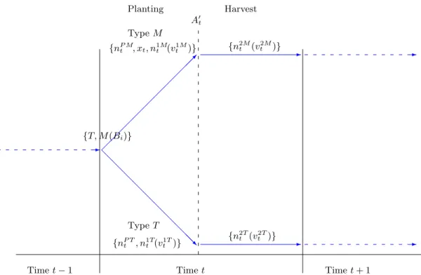
The timeline is displayed in [Figure 1.2]. Each time tis divided into two sub-periods, referred to as the
planting and harvest stages. Agents in the model are risk-neutral farmers with fixed populations and are
endowed with heterogenous ability to manage intermediate inputs: e.g., chemical fertilizer, among others.
Workers are divided into two categories, permanent and casual, and they are assumed to be perfectly
substitutable in production. An employed worker will provide a unit of labor in two successive stages if he
serves as a permanent worker or only does so at one of the stages if he is hired as a casual counterpart. In
order to reconcile fluctuations in hired labor ratios over time, casual labor is assumed to be hired through
random matching from labor markets.
Differing from the standard competitive market assumption, the matching framework gives rise to a
state-contingent matching probability in equilibrium, which is much lowered as a sharp increase in labor
demand occurs. The rationale is that the additional hiring costs serve as one possible source of labor
@ @ @ @ @ @ @ @ @@R
-Timet−1 Timet Timet+ 1
{T, M(Bi)} Planting TypeM {nP M t , xt, n1tM(v1tM)} TypeT {nP Tt , n1tT(v1tT)} A′t Harvest {n2tM(v2tM)} {n2tT(vt2T)}
market distortions, which conceptually result from how likely labor can be obtained when it is needed at
harvest time. The costs could be different across regions or over time because of labor immobility and other
distortionary factors. Hence, without prices to perfectly clear the labor market, the matching probability is
used to capture the costs based on the availability of casual labor at a certain time. Another implication
is that labor demand is likely driven by the local weather effect and the labor market is localized, so that
the matching framework could potentially better explain the large observed fluctuations in casual labor over
time or across regions.
The optimization problem that agent i faces at the beginning of the planting period at time t is to
determine a farming technology type, either modernM or traditionalT, and then production inputs
after-wards: the quantities of permanent labornP jt , casual laborn1jt andn2jt for aj-type farmer for j =M, T,
as well as the amount of intermediate inputsxtto be consumed only when he chooses to be a modern-type
agent. Accordingly, the production functions of intermediate output by modern-type and traditional-type
agents at the planting stage are respectivelyg(Bixt, nP Mt +n1Mt ) andh(nP Tt +n1Tt ), in whichBi is endowed
and individual-specific knowledge or ability to use and manage intermediate inputs. The individual-specific
ability follows a continuous distribution, say, Bi ∼ F(Bi;θ) with support in Bi = (0,∞). The ability is
augmented for intermediate inputs, and hence only takes effect when choosing modern technology.
An aggregate productivity shock A′toccurs at the beginning/end of the harvest/planting stage. Assume that the productivity shock follows a uniform distribution, A′t∼ U(µ−ε/2, µ+ε/2), and the parameterε governs the variation of the realized shock around the mean value, or the degree of uncertainty.11 Agents
cannot lay off the permanent labor that was hired from the previous stage no matter how serve the realized
shock is. There is no formal insurance available ex-ante, but after the shock is realized both types of agents
11This assumption is to facilitate the comparative statics. When dealing with computational work, other two-parameter
distributions; e.g., lnN(µA, σA) or Beta(a, b) can be alternatives to capture the effect from an enlarged degree of uncertainty
can hire additional labor, denoted asn2Mt and n2Tt . On the other hand, the available short-term contracts
for casual labor are assumed to be valid only at the current stage, i.e., either the planting or the harvest one,
and they will expire at the end of the corresponding stage. The land input ¯z is fixed and free to be used in
production.
Based on the assumptions, the production of the agricultural good for agent iis either by
FM(A′t, g(Bixt, nP Mt +n1Mt ), nP Mt +n2Mt ,z¯) =A′t[g(Bixt, ntP M+n1Mt )α(nP Mt +n2Mt )1−α]1−σz¯σ
or by
FT(A′t, h(nP Tt +n1Tt ), nP Tt +n2Tt ,z¯) =A′t[h(nP Tt +n1Tt )α(nP Tt +n2Tt )1−α]1−σz¯σ.
at the end of the harvest stage. The production functions of the intermediate output are further assumed to
beg(Bixt, nP Mt +nt1M) = (Bixt)β(nP Mt +n1Mt )1−βandh(nP Tt +n1Tt ) =nP Tt +n1Tt and remain in the CRTS
form. Final outputs are hence produced by combining land, labor to be hired at each stage, and (optional)
intermediate inputs.
Note that I only focus on the optimization problem for the current periodt, even though the framework
can be readily generalized by including dynamics on nP M
t or A′t across periods, as depicted in [Figure 1.2].
Another extension is to divide t into more than two stages, and study how agents’ discrete choices are
observed at each stage; for example, crop choosing, types of seed planting, the use of fertilizer, and irrigation
installation are sequentially affected by uninsured shocks from the future.
1.3.2
Backward solution: decisions at the harvest stage
First, consider the optimization problem for a modern-type agent withBi and solve it backwards. The
Hence, the additional value generated from hiring laborn2Mt is JM(Bi,z, A¯ ′t) = max v2M t , n2tM A′t[g(Bixt, nP Mt +n 1M t ) α(nP M t +n 2M t ) 1−α]1−σz¯σ−ξ 2v2Mt −w c tn 2M t s.t. n2Mt =ηtvt2M as A′t≥A˜ M = 0 as A′t<A˜M (1.1)
In Eq. (1.1), the amount of intermediate inputs xt and the quantity of permanent labor nP Mt have been
determined from the previous stage while n2M
t is the quantity of casual labor to be hired at the wage rate
wc
t upon creating vacancies v2Mt .
Assume that all agents are hiring labor in the market and that ηt stands for the probability that a
vacancy is filled in, which is taken as given when the agent optimizes. ξ2 denotes the additional costs paid
at the harvest stage and hencewtc+ξ2/ηtis the mean costs of hiring a unit of labor ex-post. The agent will
additionally hire labor if the realized productivity is higher than a threshold ˜AM, which is an endogenous
cut-off value that differentiates good from bad states and is a function of inputs to be determined at the
planting stage.
The optimization problem faced by traditional-type agents is analyzed under the same framework, and
their decision rules are omitted here to avoid redundance. In order to simplify the following analysis, I
assume that the only available short-term contract in the casual labor market is on take-it-or-leave-it basis
and therefore the bargaining condition can be written as
JM(Bi,z, A¯ ′t)−J¯ M =JM(B i,z, A¯ ′t)−J¯ M+ (wc t−λb)n 2M t
or
wtc=λb, (1.2)
where ¯JM equals the value of the modern-type agent from not hiring this unit of casual labor (value from
the outside option),bis disutility from providing a unit of labor in entire periodt, andλis the duration of
the harvest stage if time in the whole periodt is normalized to be one.
When the realizedA′tis larger than threshold values ˜AM and ˜AT, the first-order conditions from
modern-type and traditional-modern-type agents’ optimization problems imply that the ratios of labor inputs ex-post to
ex-ante are nP M t +n2Mt nP M t +n1Mt = {A′ t(1−α)(1−σ) [ ( Bixt nP M t +n1tM )αβ(1−σ)( z¯ nP M t +n1tM )σ] λb+ ξ2 ηt(A′t) } 1 α+σ−ασ , (1.3) and nP Mt +n2Tt nP T t +n1Tt = {A′ t(1−α)(1−σ) [ (nP Tz¯ t +n1tT )σ] λb+ ξ2 ηt(A′t) } 1 α+σ−ασ . (1.4)
Note that the matching probabilityηt=ηt(A′t) is contingent on the realized value ofA′tin equilibrium, and
that both of the ratios positively depend on the realized value ofA′tgiven the assumption that the function of the hiring costsλb+ ξ2
ηt(A′t) is concave onA
′
t. This condition is set to exclude the possibility of a dramatic
rise in marginal costs of hiring labor due to a higher value of A′t, because it may lead to a case of multiple equilibria and hence make the subsequent analysis more involved.
The endogenous threshold value ˜AM is solved by the following condition
∂FM(A′ t, g(Bixt, nP Mt +nt1M), nP Mt +n2Mt ,z¯) ∂n2M t n2M t =0 =λb+ ξ2 ηt(A′t) ,
˜
AM. Hence, the threshold ˜AM is pinned down by
˜ AM = λb+ ξ2 ηt( ˜AM) (1−α)(1−σ) {[( B ixt nP M t +n1Mt )αβ(1−σ)( z¯ nP M t +n1Mt )σ]( nP M t nP M t +n1Mt )−α−σ+ασ}−1 , (1.5)
in which the inputs xt, nP Mt , and n1Mt are given while the agent is making the decision on hiring labor
ex-post. In addition, the threshold value ˜AT from the traditional-type agent’s decision can be solved by
˜ AT = λb+ ξ2 ηt( ˜AT) (1−α)(1−σ) {( z¯ nP T t +n1Tt )σ( nP T t nP T t +n1Tt )−α−σ+ασ}−1 . (1.6)
The discrepancy between two threshold values comes from different ex-ante input combinations of the two
types of agents, and they may hence make different ex-post decisions even when facing the same aggregate
shock. Given the concavity assumption onλb+ ξ2
ηt(A′t)
, Eqs. (1.5) and (1.6) pin down unique solutions of ˜AM
and ˜AT in turn. Since the endogenous labor ratios and the threshold values rest on pre-determined input
combinations and are functions of related exogenous variables, the analysis based on comparative statics and
the underlying implications are postponed until a more detailed discussion is provided in Section 1.4.
1.3.3
Decisions at the planting stage
As presented in [Figure 1.2], agent i decides a farming technology, M or T, at the beginning of the
planting stage at timet. He then chooses the optimal quantity of permanent and casual labor to be hired
as well as the consumption of intermediate inputs if being a modern-type agent. The wage rate for hiring
a unit of permanent labor is wPt, and the labor is hired through the competitive market without creating
costly vacancies. The rationale is that permanent labor is mostly observed as family labor from the micro
data: it is paid an unobservable wage rate or directly by means of agricultural output and only minimized
costs for matching labor are required. On the other hand, in addition to wages for hiring a unit of casual
of the harvest stage.
The optimization problem of agent iis therefore outlined as
V(Bi,z¯) = max {M, T} { VM(Bi,z¯), VT(¯z) } , (1.7)
in which the value functions come from expected profits under two scenarios
VM(Bi,z¯) = max {n1M t , nP Mt , xt} { −ptxt−wPtn P M t − ( (1−λ)b+ξ1 ¯ ηc ) n1Mt +E [ FM(A′t, g(Bixt, nP Mt +n 1M t ), n P M t +n 2M t ,z¯)− ( λb+ ξ2 ηt(A′t) ) n2Mt A′t>A˜M ] +E [ FM(A′t, g(Bi, nP Mt +n 1M t ), n P M t ,¯z)A′t≤A˜ M]}. (1.8) and VT(¯z) = max {n1T t , nP Tt } { −wPtnP Tt − ( (1−λ)b+ξ1 ¯ ηc ) n1Tt +E [ FT(A′t, h(nP Tt +nt1T), nP Tt +n2Tt ,¯z)− ( λb+ ξ2 ηt(A′t) ) n2Tt A′t>A˜T ] +E [ FT(A′t, h(n P T t +n 1T t ), n P T t ,z¯)A′t≤A˜ T]} . (1.9)
The value functions indicate that, given the two endogenous thresholds solved by Eqs. (1.5) and (1.6), the
expected output is a sum of its value under the good state, which will be enlarged because of the adjustment
of the labor input ex-post, and the value under the bad state.
The first-order condition for choosingxtis
pt =E [ ∂ ∂xt { FM(A′t, g(Bixt, nP Mt +n 1M t ), n P M t +n 2M t ,¯z)− ( λb+ ξ2 ηt(A′t) ) n2Mt }A′t>A˜M ] +E [ ∂ ∂xt FM(A′t, g(Bixt, nP Mt +n 1M t ), n P M t ,z¯) A′t≤A˜M ] . (1.10)
Since the optimal quantity of labor ex-post,nP Mt +n2Mt , is a function ofxtbased on Eq. (1.3), the availability
to hire additional labor amplifies an expected marginal product ofxtunder the good state. Put differently,
the argument also implies that the demand for intermediate inputs from a modern-type agent is higher when
casual labor is available than the case in which casual labor is not available under an imposed condition
n2M
t = 0. In addition to the mean-value effect, a change in the uncertainty parameter will influence the
optimal choice ofxteven though the agent is assumed to be risk-neutral. The essence is thatnP Mt +n 2M t is
also a function of the realized stateA′t. Hence, a higher degree of uncertainty implies a higher possibility of
an extreme value ofAt occurring. This also implies that using intermediate inputs is expected to be more
productive because of an increase in the probability of ex-post adjustment under the good state. The result
is referred to as the intensive-margin effect, and under the condition that casual labor is ex-post available
the degree of uncertainty has a positive impact on the intensity of intermediate inputs relative to the others.
On the other hand, an agent with abilityBi=B, who is previously indifferent between the two technology
choices, will depart from modern to traditional technology as the uncertainty level rises. This is because
a larger share of predetermined inputs will make the value of being the modern type increase less than
the alternative, leading to the so-called negative extensive-margin effect. The two competing effects are
derived from the availability of hiring additional labor ex-post, the channel emphasized by this chapter. The
analytical results based on comparative statics and numerical exercises are shown in greater detail in the
following sections. A simplified model by imposing a relatively restricted assumption whereby labor is fully
determined ex-post is considered in the Appendix, and is used to deliver a clear sense of how the channel
gives rise to the two effects. Moreover, it qualitatively shows how a complete adjustment of the labor input
makes the adoption rate or modern technology lower as there is an exogenous increase in the degree of
1.3.4
The matching probability in equilibrium
In order to solve the state-contingent equilibrium probability that a vacancy is filled inηt(A′t), I assume
the matching function in the Cobb-Douglas form M( ¯N , Vt) = ¯mN¯ρVt1−ρ with homogeneity of degree one.
Since the part of the labor force that is available to be casual labor is ¯N in both of the planting and harvest
stages, then the number of matches rests on ¯N as well as the total vacancies created by the modern and
traditional type of agents (with fractions πM and 1−πM, respectively). Both types of agents will create
vacancies for hiring labor given thatA′t≥A˜j forj=M andT, whereas only traditional-type ones do so as
˜ AT< A′
t≤A˜M. The equilibrium probability is determined by the matching condition
ηt= ¯ mN¯ρ[(1−πM)vt2T + ∫ Bi>Bv 2M t (Bi)dF(Bi) ]−ρ if A′t≥A˜M ¯ mN¯ρ[(1−πM)v2T t ]−ρ if ˜AT ≤A′ t<A˜M, 1 if A′t<A˜T (1.11)
where ¯N is the total supply of casual labor and vt2M = n2Mt /ηt and v2Tt =n2Tt /ηt. More precisely, each
ηt(A′t) is pinned down by ηt1−ρ= ¯m ( ¯ N ¯ z )ρ{ (1−πM) ([(1−α)(1−σ)A′ t ( ¯z nP T t +n1tT )σ λb+ξ2 ηt ] 1 α+σ−ασ(nP T t +n1Tt nP T t ) −1 ) nP T t ¯ z + ∫ Bi>B ([(1−α)(1−σ)A′ t ( Bixt nP M t +n1tM )αβ(1−σ)( z¯ nP M t +n1tM )σ λb+ξ2 ηt ] 1 α+σ−ασ(nP M t +n1Mt nP M t ) −1 ) nP M t ¯ z dF(Bi) }−ρ , (1.12) as A′t ≥A˜T, andπM ≡∫
Bi>BdF(Bi) denotes the fraction of agents who have chosen modern technology
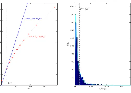
since their individual ability is larger than the threshold value B. [Figure 1.8] shows that there exists a
unique solution of equilibrium probabilityηt=ηt(A′t) in Eq. (1.12) since the left-hand side is an increasing
inηt. The comparative statics is described as ηt=ηt(A′t (−) ,n P M t ¯ z (?) ,n P T t ¯ z (?) , ξ2 (+) ),
and the details are shown in Section 1.4. First, note that an increase in nP M
t /z¯ (and nP Tt /z¯) will bring
undetermined effects on the equilibriumηt. The reasons are that (i) casual labor is perfectly substituted by
the permanent labor, and (ii) the complementarity between intermediate outputg(Bixt, nP Mt +n 1M
t ) and
total labor ex-post (nP Mt +n2Mt ) is implied by the setting of the production function. The two effects will
respectively lead agents to demand less and more casual labor ex-post, making the matching probability in
equilibrium high and low. Second, a higher realized value ofA′twill motivate agents to hire more additional labor, given that it is larger than ˜AM. Last, an exogenous increase in costs ξ
2 will dampen all agents’
incentives to hire labor ex-post, resulting in a higher matching probability in equilibrium.
The matching framework at the planting stage follows the same rule. The more detailed numerical
analysis and comparative statics and provided in the following sections and in the Appendix.
1.4
Comparative statics analysis of the generalized model
How an exogenous change in the degree of uncertainty will affect agents’ ex-ante decisions regarding
input combinations is presented in this section. The main concern is that uncertainty will only affect agents’
ex-post decisions indirectly through its effects on these input combinations.
In the generalized model, casual labor is available both before and after a productivity shock A′t is realized. The technology adoption decision of an agent with abilityBi at the beginning oft is outlined as
V(Bi,z¯) = max {M, T} { VM(Bi,z¯), VT(¯z) } ,
modern-type agent can be expressed in detail as VM(Bi,z¯) = max {n1M t , nP Mt , xt} { −ptxt−wPtn P M t − ( (1−λ)b+ξ1 ¯ ηc ) n1Mt + ∫ A¯ ˜ AM { A′t[g(Bixt, nP Mt +n 1M t )] α(1−σ)(nP M t +n 2M t ) (1−α)(1−σ)z¯σ−(λb+ ξ2 ηt(A′t) ) n2Mt } dF(A′t) + ∫ A˜M A { A′t[g(Bixt, nP Mt +n 1M t ))] α(1−σ)(nP M t ) (1−α)(1−σ)z¯σ}dF(A′ t) } . (1.13)
The expected costs of hiring a unit of casual labor is contingent on the realized value of A′t whereas the
expected costs ex-ante only rests on its distribution parameters in equilibrium. As mentioned, the endogenous
threshold value ˜AM is determined by Eq. (1.5) and it implies that the agent is indifferent between hiring
and not hiring the first unit of labor asA′t= ˜AM.
The quantity of labor to be hired ex-post by the agent as A′t ≥ A˜M, given all other predetermined
production inputs, follows the first-order condition described by Eq. (1.3). By substituting nP Mt +n2Mt in
terms of a function ofnP Mt +n1Mt into Eq. (1.13) and because of the assumptionAt′ ∼ U(µ−ε/2, µ+ε/2),
VM(Bi,z¯) = max {n1M t , nP Mt , xt} { −ptxt−wPtn P M t −((1−λ)b+ ξ1 ¯ ηc)n 1M t + ∫ µ+ε/2 ˜ AM { C(A′t)α+σ1−ασ(Bixt) αβ(1−σ) α+σ−ασ(nP M t +n 1M t ) α(1−β)(1−σ) α+σ−ασ z¯ σ α+σ−ασ + ( λb+ ξ2 ηt(A′t) ) nP Mt }1 εdA ′ t + ∫ A˜M µ−ε/2 { A′t(Bixt)αβ(1−σ)(nP Mt +n 1M t ) α(1−β)(1−σ)(nP M t ) (1−α)(1−σ)z¯σ}1 εdA ′ t, (1.14)
where the constant
C= (α+σ−ασ) [ (1−α)(1−σ) λb+ ξ2 ηt(A′t) ](1−α)(1−σ) α+σ−ασ .
The first-order conditions forn1Mt ,nP Mt , andxtcan be derived in turn by: (1−λ)b+ξ1 ¯ ηc = ∫ µ+ε/2 ˜ AM { Cα(1−β)(1−σ) α+σ−ασ (A ′ t) 1 α+σ−ασ[( Bixt nP M t +n1Mt )αβ(1−σ)( z¯ nP M t +n1Mt )σ]α+σ1−ασ } 1 εdA ′ t + ∫ A˜M µ−ε/2 { α(1−β)(1−σ)A′t[( Bixt nP M t +n1Mt )αβ(1−σ)( z¯ nP M t +n1Mt )σ]( nP Mt nP M t +n1Mt )(1−α)(1−σ)}1 εdA ′ t, (1.15) wPt = ∫ µ+ε/2 ˜ AM { Cα(1−β)(1−σ) α+σ−ασ (A ′ t) 1 α+σ−ασ[( Bixt nP M t +n1Mt )αβ(1−σ)( z¯ nP M t +n1Mt )σ]α+σ1−ασ + ( λb+ ξ2 ηt(A′t) )}1 εdA ′ t + ∫ A˜M µ−ε/2 { α(1−β)(1−σ)A′t [( Bixt nP M t +n1Mt )αβ(1−σ)( ¯z nP M t +n1Mt )σ]( nP Mt nP M t +n1Mt )(1−α)(1−σ) + (1−α)(1−σ)A′t[( Bixt nP M t +n1Mt )αβ(1−σ)( z¯ nP M t +n1Mt )σ]( nP Mt nP M t +n1Mt )−α−σ+ασ}1 εdA ′ t, (1.16) and finally, pt = ∫ µ+ε/2 ˜ AM { C αβ(1−σ) α+σ−ασ(A ′ t) 1 α+σ−ασ (nP M t +n 1M t xt )[( Bixt nP M t +n1Mt )αβ(1−σ)( z¯ nP M t +n1Mt )σ]α+σ1−ασ } 1 εdA ′ t + ∫ A˜M µ−ε/2 { αβ(1−σ)A′t (nP M t +n1Mt xt )[( Bixt nP M t +n1Mt )αβ(1−σ)( z¯ nP M t +n1Mt )σ]( nP Mt nP M t +n1Mt )(1−α)(1−σ)}1 εdA ′ t. (1.17)
Note that the first-order conditions (15)–(17) and endogenous thresholds ˜AM and ˜AT are related to the
en-dogenous input combinations Φ1=
[( Bixt nP M t +n1tM )αβ(1−σ)( z¯ nP M t +n1tM )σ]( nP Mt nP M t +n1tM )−α−σ+ασ , Φ2=n P M t +n 1M t xt , and Φ3= nP M t nP M t +n1tM
. The latter two ratios are of particular interest: Φ2is the inverse of intensity of
conditions (3) and (5) can be rewritten as nP M t nP M t +n2Mt = [ λb+ ξ2 ηt(A′t) A′t(1−α)(1−σ) ] 1 α+σ−ασ( 1 Φ1 ) 1 α+σ−ασ , (1.18) and (1−α)(1−σ)Φ1A˜M =λb+ ξ2 ηt( ˜AM) . (1.19)
As shown in [Figure 1.9a] and [Figure 1.10], the two conditions determine the unique threshold value of hiring
any casual labor, ˜AM, as well as the permanent-labor ratio ex-post. They also suggest that several factors
are responsible for the higher reliance on casual labor ex-post, one of which is an indirect effect derived from
uncertainty. Given its positive effect on the input combination Φ1(to be shown later), Eq. (1.19) and [Figure
1.9b] imply a lower threshold value ˜AM to hire labor ex-post when the agent is making decisions ex-ante
and taking a higher degree of uncertainty into account. On the other hand, Eq. (1.18) and [Figure 1.10] also
suggest a lower permanent labor ratio or higher casual labor ratio ex-post.
Using the input combinations defined above, the comparative statics will be conducted by simplifying
Eqs. (1.15)–(1.17) respectively as (1−λ)b+ξ1 ¯ ηc = ∫ µ+ε/2 ˜ AM(Φ 1,ξ2) { Cα(1−β)(1−σ) α+σ−ασ (A ′ tΦ1) 1 α+σ−ασΦ3 } 1 εdA ′ t+ ∫ A˜M(Φ 1,ξ2) µ−ε/2 { α(1−β)(1−σ)A′tΦ1Φ3 } 1 εdA ′ t, ≡f1CM(Φ1,Φ3;ε, ξ2), (1.20) wPt = ∫ µ+ε/2 ˜ AM(Φ1,ξ2) { Cα(1−β)(1−σ) α+σ−ασ (A ′ tΦ1) 1 α+σ−ασΦ3+ ( λb+ ξ2 ηt(A′t) )}1 εdA ′ t + ∫ A˜M(Φ 1,ξ2) µ−ε/2 { α(1−β)(1−σ)A′tΦ1Φ3+ (1−α)(1−σ)A′tΦ1 } 1 εdA ′ t =fM(Φ1,Φ3;ε, ξ2) +fM(Φ1,;ε, ξ2), (1.21)
where fPM(Φ1,;ε, ξ2)≡ ∫ µ+ε/2 ˜ AM(Φ 1,ξ2) ( λb+ ξ2 ηt(A′t) )1 εdA ′ t+ ∫ A˜M(Φ 1,ξ2) µ−ε/2 (1−α)(1−σ)A′tΦ1 1 εdA ′ t =wtP− ( (1−λ)b+ξ1 ¯ ηc ) , (1.22) and finally pt = ∫ µ+ε/2 ˜ AM(Φ1,ξ2) { C αβ(1−σ) α+σ−ασ(A ′ tΦ1) 1 α+σ−ασΦ2Φ3 } 1 εdA ′ t+ ∫ A˜M(Φ 1,ξ2) µ−ε/2 { αβ(1−σ)A′tΦ1Φ2Φ3 } 1 εdA ′ t ≡fxM(Φ1,Φ2, Φ3;ε, ξ2). (1.23)
Note that the three input combinations are jointly determined by Eqs. (1.20), (1.21), and (1.23), and hence
their values will not be functions of the individual ability level. In addition, Eq. (1.22) delivers the tradeoff
between hiring permanent and casual labor at the planting stage, since it means that the relative labor costs,
as denoted by the right-hand side of the second equality, equal the sum of the expected marginal products
under the good state A′t ∈( ˜AM, µ+ε/2) and the bad state A′t∈ (µ−ε/2,A˜M). Because of the assumed
perfect substitution between permanent and casual labor it can be shown that
wPt ≤ ( (1−λ)b+ξ1 ¯ ηc ) +E [ λb+ ξ2 ηt(A′t) ] = ( (1−λ)b+ξ1 ¯ ηc ) + ∫ µ+ε/2 µ−ε/2 ( λb+ ξ2 ηt(A′t) ) dF(A′t), (1.24)
where the inequality comes from the loss of flexibility under the bad state when deciding to hire one unit of
the permanent labor instead of one unit of casual substitute at both stages. Secondly, by comparing the two
large parentheses of Eq. (1.23), it can be shown that the marginal product of intermediate inputs (or sunk
investments) is enlarged under the good state since 1/(α+σ−ασ)>1. This is because the adjustment of the labor input is available and it makes intermediate inputs become more productive.
Since uncertainty is represented by the parameter ε and it governs the amount of variation within the
unform distribution, the comparative statics of uncertainty on the input combination Φ1 is written as
dΦ1/dε= −∂fM P /∂ε ∂fM P /∂Φ1 . (1.25)
Applying Leibniz’s rule, I can derive
∂fM P ∂ε = 1 2 [ λb+ ξ2 ηt(µ+ε2) ]1 ε−(− 1 2) [ (1−α)(1−σ)(µ−ε 2)Φ1 ]1 ε + ( −1 ε ){ ∫ µ+ε/2 ˜ AM(Φ1,ξ2) ( λb+ ξ2 ηt(A′t) )1 εdA ′ t+ ∫ A˜M(Φ 1,ξ2) µ−ε/2 (1−α)(1−σ)A′tΦ1 1 εdA ′ t } = (1 ε ){1 2 [ λb+ ξ2 ηt(µ+ε2) ] +1 2 [ (1−α)(1−σ)(µ−ε 2)Φ1 ] −fPM } T 0, (1.26) and ∂fM P ∂Φ1 = ∂ ˜ AM ∂Φ1 { (1−α)(1−σ) ˜AMΦ1− ( λb+ ξ2 ηt( ˜AM) )}1 ε+ ∫ A˜M µ−ε/2 (1−α)(1−σ)A′t 1 εdA ′ t = ∫ A˜M µ−ε/2 (1−α)(1−σ)A′t1 εdA ′ t>0. (1.27)
The second equality of Eq. (1.27) is derived by using the determination condition of ˜AM based on Eq. (1.19)
and the positive, equal, or negative sign of Eq. (1.26) rests on the concavity, linearity or convexity of the
functionλb+ ξ2
ηt(A′t) onA
′
t, respectively. Hence, I have dΦ1/dε > 0 if the costs of hiring, λb+ ηtξ(A2′
t), are
concave onA′t, as shown in [Figure 1.9a]. The assumption implies that the hiring costs do not increase too dramatically and hence excludes the possibility of multiple equilibria and less reliance on casual labor under
high-productivity realizations. Because the threshold value ˜AM is lowered as the degree of uncertainty rises,
the resultdA˜M/dε <0 implies that the rising uncertainty will increase the extent of reliance on casual labor.
In order to understand the influence of uncertainty on the share of permanent labor at the planting stage
dΦ3/dε=− ∂fM 1C/∂ε + (∂f1CM/∂Φ1)(dΦ1/dε) ∂fM 1C/∂Φ3 (1.28)
by using Eq. (1.20) and givendΦ1/dε >0 with
∂fM 1C ∂ε = 1 ε { 1 2C [α(1−β)(1−σ) α+σ−ασ ]( (µ+ε 2)Φ1 ) 1 α+σ−ασ Φ3+ 1 2α(1−β)(1−σ)(µ− ε 2)Φ1Φ3− [ (1−λ)b+ξ1 ¯ ηc ]} >0, (1.29) ∂f1CM ∂Φ3 = [ (1−λ)b+ξ1 ¯ ηc ] 1 Φ3 >0, (1.30) and ∂fM 1C ∂Φ1 > [ (1−λ)b+ξ1 ¯ ηc ] 1 Φ1 >0. (1.31)
The comparative statics shows that dΦ3/dε < 0 and hence the casual-labor ratio at the planting stage, n1M
t
nP M t +n1tM
= 1−Φ3, is increasing in the degree of uncertainty. Moreover, the casual-labor ratio at the harvest
stage, n2tM
nP M t +n2tM
, is also increasing in the degree of uncertainty because of Eq. (1.18) anddΦ1/dε >0, which
hinges on the assumption that the marginal costsλb+ ξ2
ηt(A′t) are concave onA
′
t.
Finally, the comparative statics of the ratio of labor ex-ante to intermediate inputs with respect toεis
dΦ2/dε=
∂fxM/∂ε−(∂fxM/∂Φ1)(dΦ1/dε)−(∂fxM/∂Φ3)(dΦ3/dε)
∂fM x /∂Φ2
, (1.32)
which is derived by using Eq. (1.23) and its components are
∂fxM ∂ε = 1 ε { 1 2 [ C αβ(1−σ) α+σ−ασ ( (µ+ε 2)Φ1 ) 1 α+σ−ασ Φ2Φ3 ] +1 2 [ αβ(1−σ)(µ−ε 2)Φ1Φ2Φ3 ] −pt } >0 (1.33) and ∂fxM ∂Φι = pt Φι >0 forι= 1,2,3. (1.34)