Sibling Health, Schooling and
Longer-Term Developmental Outcomes
Chris Ryan
Melbourne Institute of Applied Economic and Social Research, The University of Melbourne
Anna Zhu
Melbourne Institute of Applied Economic and Social Research, The University of Melbourne
No. 2016-15 July 2016
NON-TECHNICAL SUMMARY
We explore the extent to which starting primary school earlier by up to one year can help shield children from the detrimental, long-term developmental consequences of having an ill or disabled sibling. Primary school entry age is an adjustable policy tool. Over the last few decades, the legal minimum age of school start has gradually increased in most developed nations. Deming & Dynarski (2008) attribute roughly a quarter of this upward drift in the age at which children are allowed to start primary school in the United States, for example, to changes imposed by the state. This policy direction has broadly been motivated by the intention to increase the school readiness of children. The actual benefits of delaying school start are not, however, unambiguously positive. Particularly for disadvantaged children, spending additional time out of school may in fact be unhelpful compared to starting school at an earlier age. Importantly, children who delay their school entry may linger in environments whose quality is positively correlated with their parent's time and money resources. Entering school earlier, by contrast, may work to equalise the opportunities to learn and interact because it asymmetrically increases a relatively disadvantaged child's exposure to educational stimulation.
We have chosen to focus on the presence of an ill sibling rather than on more conventional measures of disadvantage. Most of the literature evaluating major early childhood programs use the more conventional measures of income poverty or the child's own human capital endowments and find that the benefits for children's cognitive achievement scores tend to fade-out quickly. These programs usually target deeply disadvantaged children whose experiences of hardship are often multi-faceted and continue to affect them long after they complete the programs. The depth of their disadvantage may thus undermine the ability of these children to capitalise on the initial gains from program participation. In contrast, the existence of poor health in the sibling may be a less entrenched source of disadvantage than poverty or the study child's own low IQ. Even though poor health in the sibling may entail and partly originate from broader experiences of economic and social disadvantage, there is also an element of bad luck when it comes to how poor sibling health is distributed among families.
Using data from the Longitudinal Study of Australian Children, we find that Australian children who have a sibling in poor health persistently lag behind other children in their cognitive development - but only for the children who start school later. In contrast, for the children who commence school earlier, we do not find any cognitive developmental gaps. The results are strongest when the ill-health in the sibling is of a temporary rather than longer-term nature. However, we find mixed impacts on the gaps in non-cognitive development.
ABOUT THE AUTHORS
Chris Ryan commenced as Director of the Economics of Education and Child Development program at the Melbourne Institute in April 2011. His research interests span the determinants of and outcomes from participation in different types of education, the impact of related government programs and interventions, and the transitions of young people from education and training into the labour market. Email:
ryan.c@unimelb.edu.au.
Anna Zhu’s research uses econometric techniques combined with national survey and administrative datasets to investigate issues on child development, the intergenerational transmission of disadvantage, childhood homelessness or maltreatment and employment. She is also a research fellow of the ARC Centre of Excellence’s Life Course Centre and a research affiliate at the Institute for the Study of Labor (IZA). Email: anna.zhu@unimelb.edu.au.
ACKNOWLEDGEMENTS: This research was supported by the Australian Research Council (ARC) Centre of Excellence for Children and Families over the Life Course (project number CE140100027). The Centre is administered by the Institute for Social Science Research at The University of Queensland, with nodes at The University of Western Australia, The University of Melbourne and The University of Sydney. This paper uses unit record data from Growing Up in Australia, the Longitudinal Study of Australian Children. The study is conducted in partnership between the Department of Social Services (DSS), the Australian Institute of Family Studies (AIFS) and the Australian Bureau of Statistics (ABS). The findings and views reported in this paper are those of the authors and should not be attributed to the ARC, DSS, AIFS or the ABS. The paper benefited from the helpful comments of: Bruce Bradbury, Liz Washbrook, David Ribar and the attendees of the Melbourne Institute Brown-bag seminar and the attendees of the Social Policy Research Centre external seminar. All opinions and any mistakes are our own.
DISCLAIMER: The content of this Working Paper does not necessarily reflect the views and opinions of the Life Course Centre. Responsibility for any information and views expressed in this Working Paper lies entirely with the author(s).
(ARC Centre of Excellence for Children and Families over the Life Course) Institute for Social Science Research, The University of Queensland (administration node)
UQ Long Pocket Precinct, Indooroopilly, Qld 4068, Telephone: +61 7 334 67477 Email: lcc@uq.edu.au, Web: www.lifecoursecentre.org.au
Abstract
We explore the extent to which starting primary school earlier by up to one year can help shield children from the detrimental, long-term developmental consequences of having an ill or disabled sibling. Using data from the Longitudinal Study of Australian Children, we employ a Regression Discontinuity Design based on birthday eligibility cut-offs. We find that Australian children who have a sibling in poor health persistently lag behind other children in their cognitive development - but only for the children who start school later. In contrast, for the children who commence school earlier, we do not find any cognitive developmental gaps. The results are strongest when the ill-health in the sibling is of a temporary rather than longer-term nature. We hypothesise that an early school start achieves this by lessening the importance of resource-access inequalities within the family home. However, we find mixed impacts on the gaps in non-cognitive development.
Keywords: educational economics, human capital, school starting age, sibling health
1
Introduction
Early childhood education programs have the potential to close student achievement gaps between disadvantaged children and their relatively advantaged peers (Heckman 2006; Raudenbush & Eschmann 2015). For many programs, researchers find that certain groups of disadvantaged children derive greater benefits than other groups, especially in the longer term (Garces, Thomas & Currie 2002; Conti, Heckman & Pinto 2015). Identifying the groups of children who particularly benefit from a given program is important. It can improve both our targeting efforts as well as our understanding of human capital development and the ingredients of a program that facilitate this in effective and enduring ways.
In this paper, we identify a group of disadvantaged Australian children who catch up and maintain parity, in student achievement scores, with their relatively advantaged peers because of the timing of their primary school entry. Primary school entry age is an adjustable policy tool. Over the last few decades, the legal minimum age of school start has gradually increased in most developed nations. Deming & Dynarski (2008) attribute roughly a quarter of this upward drift in the age at which children are allowed to start primary school in the United States, for example, to changes imposed by the state. This policy direction has broadly been motivated by the intention to increase the school readiness of children.
The actual benefits of delaying school start are not, however, unambiguously positive (Black, Devereux & Salvanes 2011). Particularly for disadvantaged children, spending additional time out of school may in fact be unhelpful compared to starting school at an earlier age. Importantly, children who delay their school entry may linger in environments whose quality is positively correlated with their parent’s time and money resources. En-tering school earlier, by contrast, may work to equalise the opportunities to learn and interact because it asymmetrically increases a relatively disadvantaged child’s exposure to educational stimulation (Raudenbush & Eschmann 2015).
One group of children who may benefit from an early school start are those who have a sibling in poor health since they are likely to face large resource (and thus learning) constraints in the family home. Indeed, researchers find that children who have a sibling in poor health tend to receive less parental attention, are read to less often and are more likely to interact with stressed parents (Dyson 1996; Parish & Cloud 2006; Mulroy, Robertson, Aiberti, Leonard & Bower 2008; Antonopoulou, Hadjikakou, Stampoltzis & Nicolaou 2012; Allin & Stabile 2012). They also tend to have poorer social and economic
outcomes in the short and longer term compared to children who do not have ill or disabled siblings (Fletcher, Hair & Wolfe 2012; Rossiter & Sharpe 2001).
Our interest is not, however, to identify the causal effect of the sibling’s poor health on a child’s developmental outcomes. Instead, we use the indicator to identify children who may experience some form of constraint on resource-access within the home environment. Young children with a sibling in poor health are compared to other children who, at the same age, did not have any family member with poor health. Their cognitive and non-cognitive developmental gaps are further compared across groups of children who happen to start school “earlier” (by up to one year) and those who start school “later”. We use a Regression Discontinuity Design based on birthday eligibility cut-offs to mirror randomisation in the the timing of school entrance.
We have chosen to focus on the presence of an ill sibling rather than on more conventional measures of disadvantage. Most of the literature evaluating major early childhood pro-grams use the more conventional measures of income poverty or the child’s own human capital endowments and most find that the benefits for children’s cognitive achievement scores tend to fade-out quickly (Duncan & Magnuson 2013). These programs usually tar-get deeply disadvantaged children whose experiences of hardship are often multi-faceted and continue to affect them long after they complete the programs (Garces, Thomas & Currie 2002). The depth of their disadvantage may thus undermine the ability of these children to capitalise on the initial gains from program participation.
In contrast, the existence of poor health in the sibling may be a less entrenched source of disadvantage than poverty or the study child’s own low IQ. Even though poor health in the sibling may entail and partly originate from broader experiences of economic and social disadvantage, there is also an element of bad luck when it comes to how poor sibling health is distributed among families. For example, while children from the highest and lowest income quintiles at age five have a vocabulary achievement gap of 0.85 of a standard deviation (Bradbury, Corak, Waldfogel & Washbrook 2012), it is far smaller between children with and without a sibling in poor health, at roughly one quarter of a standard deviation.
In our data, we can further distinguish between poor health in a sibling that is of a temporary versus a longer term nature. Children whose sibling has a temporary health condition may experience less disruption or they may live in families that are better equipped to address the health condition of the sibling. Nevertheless, even short duration health ‘shocks’ in the family can have enduring negative impacts on children’s achievement
scores (Hull 2014) if they divert children onto less productive learning paths (Cunha & Heckman 2007).
Our results are consistent with this observation. We find that children who have siblings with a temporary illness are indeed penalised in the longer term - but only for the children who start school late. For the children who start school early, the cognitive development gap is non-existent. This suggests that the effectiveness of early educational programs in closing developmental inequalities may depend on the type of and persistence in pre-existing inequalities.
Put differently, our results also highlight the existence of important heterogenous impacts of starting school earlier, by the degree of disadvantage experienced by the child. For this reason, we depart from the economics of education literature that largely explores the impact of school starting age in its own right (Datar 2006; Elder & Lubotsky 2009; Black, Devereux & Salvanes 2011; Fleury 2011; and Pellizzari & Billari 2012). Instead, our paper aligns closely to the research focusing on the heterogenous impacts (Cascio & Lewis 2006; Hamori & Kollo 2011 and Suziedelyte & Zhu 2015).
We extend this research agenda, however, in two main ways. Using nationally representa-tive data from the Longitudinal Study of Australian Children (LSAC), otherwise known asGrowing Up in Australia, we assess a range of child cognitive outcomes based on both survey responses and administrative-based, nation-wide literacy and numeracy test scores called the National Assessment Program - Literacy and Numeracy or NAPLAN. We also have non-cognitive outcomes that are reported by the parent as well as by the teacher. As we observe child outcomes throughout time, we are able to explore the developmental trajectories of children as they transition from the beginning of primary school into late childhood or early teenage years. An additional contribution we make to the literature is that we explore why starting school early by up to one year can help children with a sibling in poor health to maintain developmental parity with other children both in the short and longer term.
We argue the reasons are two-fold. First, entering school can be more beneficial for chil-dren who face constraints on learning in the family home compared to those who already have educationally enriching home environments. Although schools differ in quality, most children who attend Australian schools have access to resources such as the school library, peer interactions, mentorship, play equipment, and adult attention. At the very least, they have access to 30 hours per week of structured time that is intended to help them to learn.
Related to this, substitution of school for home may also lessen the importance of re-maining inequalities in resource-access within the family home. When children receive a higher base level of educational stimulation, such as the amount they are read to, addi-tional reading within the home may matter less. Here, we view the gains to such home inputs as being likely subject to diminishing returns and child development following a standard production process that is concave in hours of cognitive stimulation, what-ever their source. We indeed find that differences in cognitive inputs within the home environment matter less for children who are in school compared to those who are not. Second, when children receive schooling at a younger age, they can derive greater de-velopmental gains. Evidence in the economics and neuroscience literatures points to the ‘earlier is better’ pattern of effect for children’s later life outcomes (Sapolsky 2004; Nelson & Sheridan 2011; and Chetty, Hendren & Katz 2015). The argument is that children tend to derive larger benefits from an earlier intervention because of the greater plasticity in their cognitive and language abilities - their skills are more amenable to environmental en-richment. Further, when children gain critical skills early in life, their capacity to benefit from further skills development is greater - given the concept of dynamic complementarity (Heckman 2006).
In the next section, we describe Australia’s education system briefly. Section 3 contains a description of the data used and Section 4 outlines the methodology. The results are presented in Section 5, and explored in more detail in Sections 6, where we assess how the impact of different types of home inputs on child development is affected by starting school early. Section 7 tests the robustness of our results and Section 8 concludes.
2
Australia’s Education System
The school starting rules in Australia are based on when a child was born relative to a state-specific, cut-off eligibility date. Children born before the cut-off are eligible to start school in the year that they turn five years old, whereas children born after the cut-off are expected to begin school in the following year. In most states in Australia, there is only one school intake per year (in late January or early February). In this paper, we focus on the following four states and territories: New South Wales (NSW), Victoria (VIC), the Australian Capital Territory (ACT) and Western Australia (WA) because the primary school start rules for these four states are similar.1 These states have the following cut-off dates: 31 July for NSW, 30 June for WA and 30 April for VIC and the ACT. Thus, these
1We exclude South Australia and Northern Territory because they had a rolling admission policy
rules segment children into those who are eligible to start school “early” and those who are not. We consider early entrant children as those born in the first “part” of the year (January to July in NSW, January to April in VIC/ACT, and January to June in WA), and late entrant children are those born in the second “part” of the same calendar year. In practice, however, our data only capture children born from March 1999 onwards; we discuss this later in more detail.
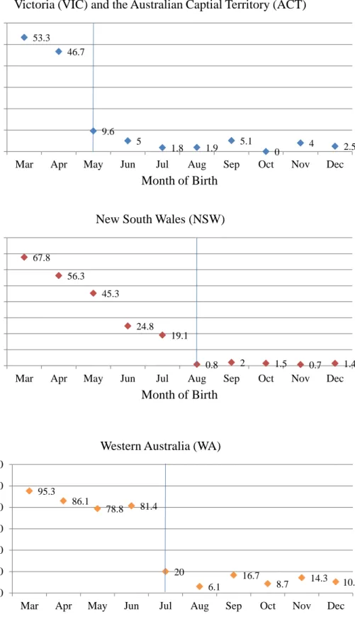
We show that school entry rules in Australia indeed affect the actual timing of school entry - Figure 1 plots the percentage of children who are in school in our data by their month of birth. Since our sample of children was born in the same year (1999), the month of birth also represents the month of the year in which the child turns five. Figure 1 shows that the school entry rules affect the timing of school start for children from all states, however, there are differences in the compliance rates across these states. In WA, compliance with the school entry rules is the greatest. At the cut-off, the percentage of children who are in school decreases from 81 percent to 20 percent. In VIC/ACT, compliance with school entry rules is also substantial with the percentage of children in school decreasing from 47 percent for the children born just before the cut-off to 10 percent for children born just after the cut-off. By contrast, in NSW compliance with the school entry rules is weak with the percentage of children attending school decreasing from 19 percent to less than one percent at the cut-off.
These rules mean that some children commence school up to one year earlier than others in a random fashion (insofar as the timing of birth is random, which we will test later). We explain in the method section how we disentangle the age of school start effect from the age-at-test (or years of schooling) effect. For children who are born after the cut-off (and thus start school later), this implies spending longer in the family home or in child care than children who are born before the cut-off (and thus who start school earlier). For the majority of children, this means spending longer in the family home, even if they also used centre-based child care. One reason for this is because Australian mothers have a tendency to return to work only until their youngest child begins primary school (Zhu & Bradbury 2015). Further, state-provided preschool is usually only offered to children for up to 15 hours per week, thus for the majority of the time that children are waiting to enter school, we may still expect them to be in informal care or within the family home. Students who are Australian citizens and permanent residents can (largely) attend Gov-ernment (public) schools for free, whereas Catholic and independent (private) schools usually charge attendance fees. However, the private schools are also subsidised by the
cohort experienced a year of “transition” arrangements, and we also exclude Tasmania as its students enter school at a later age than children in other states.
state and federal governments, thus in this paper we refer to public investments as both forms of schooling. Across Australia, Government schools educate approximately 65 per cent of Australian students, with the balance in Catholic and independent schools. Re-gardless of the type of system, schools in Australia are largely required to adhere to the same curriculum frameworks of their state or territory.
3
Data
The data used in this paper are based on the Longitudinal Study of Australian Children (LSAC) - a nationally representative longitudinal survey of Australian children and their families conducted every two years beginning from 2004. We analyse a cohort of children born from March to December 1999, known as the “K-cohort”. The available data allow us to examine the effect of early school start (at ages four-to-five years) on children’s outcomes from the age of 6 through to 11 years old, with two-year gaps in between i.e. we analyse four waves of data. As previously mentioned, our sample of children attend school in the following four States or Territories of Australia: NSW, VIC, the ACT and WA.
We analyse a balanced panel (children who are present in all four waves) in order to ensure estimated developmental gaps do not arise from changing sample compositions. The wave 1 to wave 4 attrition rate in our sample is approximately 34 percent. However, we do not find that the propensity to attrit is correlated with the control variables included in the main regression, specifically the indicator for disability in a household member, state indicators, the early start school eligibility indicator and child age indicators as measured at wave 1. The p-value on the Wald test of the joint significance of these variables in the regression against whether individuals drop out or not is 0.37. We also find that the propensity to drop out of the study in later waves is unrelated to the early child development outcomes. Using wave 2 scores as the outcomes of interest, we re-estimate the results for the families who were present in waves 1 and 2 and dropped out in either waves 3 or 4 (consisting of 441 person observations) and compare the results to those who stayed in the survey for all four waves. We find that the results are substantively similar across these two samples.
The LSAC data include a wide array of variables on children’s cognitive and non-cognitive outcomes. We describe these in detail in the next sub-section. We have both parent and teacher reported developmental indicators, although there are fewer observations for teacher responses, as some of the surveys sent to the teachers of children were not
re-turned. The sample size is more than 1,700 children (for parent responses), and just over 1,600 children (for teacher responses).2 Further, our survey data are linked to administrative data on national test scores based on the National Assessment Program -Literacy and Numeracy. Results using the NAPLAN scores are based on approximately 1,450 children.
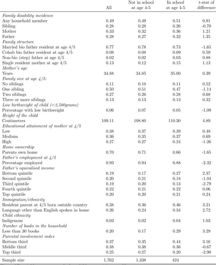
In Table 1, we provide descriptive statistics on the sample at age four to five years old, by the early school start status. There are some clear demographic differences between children who start school early versus later. For example, the parents of the former are more likely to be overseas-born and from a non-English speaking background than the parents of the latter. They also tend to come from families with lower socioeconomic status, where the home ownership rates are lower, fathers are less likely to be employed and more likely to earn a low level of income. Further, these children receive lower levels of exposure to home or parental investments, as measured by the number of books at home and parental involvement in child activities. These differences in the family and child characteristics by early school start status show that the school starting age is unlikely to be exogenous. In the method section, we explain how we exploit school starting rules to derive exogenous variation in the school starting age.
3.1
Children’s Developmental Outcomes
Children’s cognitive aptitude is measured by achievement test scores that are admin-istered to the child at the time of the survey. We also have teacher responses in the survey as a point of contrast. For survey-based assessments, we use the test scores of the Peabody Picture Vocabulary Test (PPVT), and the Matrix Reasoning test. For the teachers, we use the Academic Rating Scale (ARS) for Language and Literacy and sepa-rately for Mathematical thinking, as well as an index measuring the child’s approach to learning.
The PPVT is a test designed to measure a child’s knowledge of the meaning of spoken words and his or her receptive vocabulary for Standard American English, with a number of changes made for greater applicability to the Australian context. The PPVT entails the interviewer showing the child a book with 40 plates of display pictures and where the child points to (or says the number of) a picture that best represents the meaning of the word read out by the interviewer. The items in this test change to reflect an appropriate difficulty for the respective ages of the children tested. The Matrix Reasoning test is based
2The sample varies depending on the indicator of poor sibling health used - we consider the base
on the Wechsler Intelligence Scale for Children. It tests the child’s problem solving ability by presenting children with an incomplete set of diagrams and requiring them to select the picture that completes the set from five different options. The instrument comprises 35 items of increasing complexity and the child starts on the item that corresponds to his/her age-appropriate start point.
Teachers are asked to complete the ARS - Language and Literacy (and mathematical thinking) questionnaires, which rate the child’s language and literacy skills (and mathe-matical thinking abilities) in relation to other children of the same age. The approach to learning index comprises questions that rate a child’s: organisational ability, eagerness to learn new things, independence, ability to adapt to changes in routine and his/her persistence in completing tasks.
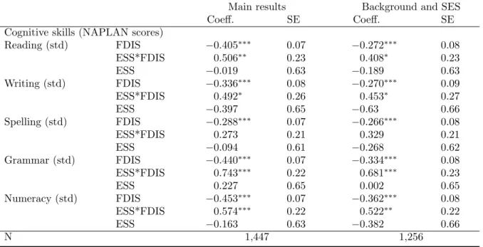
The last set of cognitive outcomes we use is based on administrative data from the NAPLAN test scores. NAPLAN is a nation-wide, annual assessment for students in Years 3, 5, 7 and 9, and was introduced in 2008. It provides point-in-time information on students’ progress in literacy and numeracy and is made up of tests in four domains including: reading, writing, language conventions (spelling, grammar and punctuation) and numeracy. We present the test results for Years 5 and 7 - there are many missing observations for the Year 3 sample since NAPLAN was introduced after many children in our sample had completed Year 3, while the Year 9 results were unavailable at the time of this study.
The non-cognitive skills are measured by a child’s behaviour problems as identified in the parent and teacher responses to the Strengths and Difficulties Questionnaire (SDQ). There are five sub-scales of the SDQ, namely, Hyperactivity, Emotional, Peer problems, Pro-social and Conduct problems. Within each of these five sub-scales, parents are asked five questions and for each specific question they rate whether the incidence of child be-havioural issues is “never true”,“somewhat true” or “certainly true” of a child. Some examples of behavioural issues are “fights with other children”, “spiteful to others” and “argumentative with adults”. We treat the child as exhibiting the specific behavioural issue if parents answer either “certainly true” or “somewhat true” to the specific question. We argue that transforming these variables into this binary form, as opposed to making a distinction between the “certainly true” and “somewhat true” responses, imposes a less arbitrary assessment of the extent to which the child exhibits the specific behavioural problem (Dix, Askell-Williams & Lawson 2008). Based on these five sub-scales, we con-struct three separate measures of non-cognitive skills - (1) internalising behaviours, which combines the emotional and peer sub-scales; (2) externalising behaviours, which combines the hyperactivity and conduct problems sub-scales; and (3) pro-social skills. The
inter-nalising and exterinter-nalising behaviour indices are reverse coded so that a higher value indicates a higher level of a non-cognitive skill (or less problematic behaviour).
For all of our cognitive and non-cognitive outcomes, we standardise them with respect to the weighted sample mean and standard deviation. Thus, the weighted means of these outcomes are equal to zero and their standard deviations are equal to one.
3.2
Family Illness and Disability Measures
We consider a family member to have an illness or disability if the response to the question: “does...have any medical conditions or disabilities that have lasted, or are likely to last, for six months or more?”, is yes. The survey also records the name and relation of the person to the study child for each wave and thus we are able to gauge which family member was in poor health across the waves. But for our main variable of interest, we only use information from wave one, when the study child is aged four to five years, to see if they were living with an ill or disabled family member at that time.
We create separate indicators of ‘poor health in the family’ for the illness or disability of: any sibling, the mother and the father. Yet, our focus in this paper is on poor health in the sibling. The base case for all of these indicators is that there is no family member with a disability. This necessarily leads our samples to differ depending on which family member we focus on. Based on the above definition, we find that a substantial number of children had a family member who was disabled or who had a long term health condition (lasting or expected to last for six months or more) when they were aged four to five years. 28 per cent had such a sibling, 33 per cent a mother and 28 per cent a father. In aggregate, 49 per cent had such a family member.
Thus, our definition of illness and disability is a broad one and captures a relatively higher incidence of illness and disability compared to other surveys. For example, the Household, Income and Labour Dynamics in Australia (HILDA) survey estimates the incidence of disability in the family to be 18 per cent and the Survey of Disability, Aging and Caring (SDAC) based on Australian Bureau of Statistics (ABS) data (2009) estimates it to be 19 per cent. The reality is that there is no one agreed-upon definition of disability - not in the literature, nor in practice - and the different criteria used to identify persons with a functional limitation yield dramatically different rates (UNICEF 2013). For example, the SDAC asks the respondent if anyone in the household has any of 17 different types of medical conditions, which is more specific than the LSAC survey, which more broadly asks if there is ‘any’ medical condition or disability that has lasted or is likely to last for six months or more. Unfortunately, the LSAC survey does not ask about the everyday
impairment associated with the family member’s illness or disability for the K-cohort during the first wave.
Nevertheless, we hypothesis that when children live with a family member with an illness or disability during critical stages of development they can be penalised in the longer term. We consider the years four to five to be a critical age for children’s development and hypothesis that it is sensitive to shocks in the family, even if the illness of the family member is transitory. Our main definition of illness or disability in the family includes those that are relatively long-term as well as transitory.
As a sensitivity analysis, we later distinguish between the types of illnesses or disabilities in the sibling that are transitory versus longer-term. We consider siblings to have a longer-term disability if we observe them to have the illness or disability for both waves 1 and 2 (when children are aged four-to-five to six-to-seven). Consequently, the incidence rates drop to 19 per cent for any family member; 12 per cent for a sibling; 15 per cent for a mother; and 31 per cent for a father.3 We continue to define the base case as a child, who at age four-to-five (in wave 1), was without ‘any’ ill or disabled family member. We exclude families who reported having an ill or disabled family member in wave 2 but not in wave 1 from the base group. We consider a sibling to have a transitory illness or disability if we observe them to have it for only wave 1 (and not in wave 2).
4
Methods
Our main aim is to test whether an early school start can narrow the gap in cognitive and non-cognitive skills between children with and without an ill or disabled sibling. Put differently, we wish to test for any heterogenous impacts (of an early school start) between them. We can explore this in a standard Ordinary Least Squares (OLS) setting by estimating the following linear regression for each skill k:
sk,i =γ0k+γ1kESSk,i+γ2kF DISk,i+γ3kESSk,i∗F DISk,i
+γ4kf(AGE)k,i+Xk,i0 γ5k+γ6kf(AGE)k,i∗Xk,i0 +vk,i, (1)
whereESS equals to one if the child started school early (by up to one year) i.e. he/she started at age four-to-five and zero otherwise. F DIS equals to one if the child had a sibling (and later, mother and father) with an illness or disability and zero otherwise.
3The incidence for fathers actually increases using this stricter definition because the sample attrition
from waves 1 to 2 for fathers is disproportionately higher among fathers who never report having an illness or disability.
Our main variable of interest is the interaction of ESS and F DIS. In our set-up, both groups of children who do and do not have an ill or disabled sibling receive the treatment of an early school start, however, we hypothesise that they derive different levels of benefit from it. The vectorX includes state of residence dummies for NSW (base category), WA and VIC and ACT combined (since the rules in the latter two are identical). f(AGE) is a flexible, non-parametric function of the running variable of child age, which we outline in more detail below, interacted with the state of residence. The error term is denoted as vk,i.
Cognitive and non-cognitive skills are measured at ages 6-7, 8-9, and 10-11 and Years 5 and 7 for the NAPLAN scores. The parameter γ2k is interpreted as the gap in a skill k between children with and without an ill or disabled sibling in the sub-sample of late school starters (ESS = 0). Whereas the gap between children with and without an ill or disabled sibling, in a skill k, for the early school starters is calculated as: γ2k +γ3k.
Thus, we can interpret the parameter γ3k as how much an early school start closes (or
widens) these developmental gaps. An alternative interpretation is how the ESS effect varies by F DIS status i.e. the parameter γ1k is the effect of an early school start for
children without an ill or disabled sibling (F DIS = 0) and the effect of an early school start for children with an ill or disabled sibling is calculated as γ1k+γ3k.
4.1
Potential Endogeneity
The identification of the parameters in equation (1) is complicated by the potential en-dogeneity of: the F DIS status, ESS as well as the interaction of these two variables. Thus, estimating equation (1) by OLS may result in biased coefficient estimates.
In this paper, we are mainly concerned with potential endogeneity with the early school start variable, that is, the correlation between ESSk,i and vk,t. Parents may decide to
delay a child’s entry to school if, for example, the child has weaker cognitive or non-cognitive skills. Moreover, our estimate ofγ3kmay be biased if children with an ill sibling
are more (or less) likely to be held back from starting school in the year they turn five compared to their peers. Such differential compliance makes it difficult to disentangle differential effects of an early school start from differences in the composition of early school starters across those with and without an ill sibling.
Endogeneity in F DIS primarily matters for how we interpret the results. Specifically, it matters for ‘why’ an early school start may close gaps. To take an extreme example then, assume that the illness in the sibling arises entirely from income poverty and assume that an early school start can narrow developmental gaps (i.e. a positive γ3k). The main
reason income poor children may benefit from an early school start may be because of the income replacement effect (as the mother can return to work earlier). In addition, the school environment may be more enriching than the environment in an income-poor household. Both of these factors may contribute to the estimates we observe. When we target an early school start at children with ill siblings (whom in this scenario are also income poor), it will help them to catch up to their advantaged peers regardless of the original cause of their disadvantage. Thus our immediate interest is not to identify the causal effect of poor health in the child’s sibling.
However, for interpretation purposes, we try to minimise endogeneity associated with F DIS in our sensitivity analysis. The estimate of γ3k will off-set endogeneity in F DIS
for sources that are constant across early and late school starters. We address potential endogeneity in F DIS in two additional ways. First, we identify temporary forms of poor health in the sibling, which are more likely to indicate a health shock in the family. Second, we control for an array of background controls. This can help us to identify the disruption uniquely produced by poor health in the sibling over and above other correlated sources of disadvantage.
4.2
Identifying Variation and Implementation
To address endogeneity inESS, we rely on two sources of exogenous variation to identify the direct effect for the two distinct groups of children - those with and without an ill or disabled sibling. The first source is generated by the Australian school entry regulations. These policy features mean that children born just prior to the cut-off date can start school up to (nearly) one year earlier than children born just after the cut-off date - yet we expect them to be very similar along all background characteristics. The probability of going to school early jumps discontinuously (as we later show) at the cut-off points4 but it is not solely determined by the strict cut-off rule. As previously mentioned, a high percentage of children in our sample are held back or ‘red-shirted’ - they do not enter school in the year they are eligible. Thus we use a fuzzy regression discontinuity design (RDD) framework.
The second source of identifying variation we use is across school or state starting times. As outlined in Section 2, the cut-off rule varies across states. For example, if we have two children who turn five years old on the same day (say May 15), but one lives in Victoria and the other one lives in New South Wales, the first one will be not eligible to go to school that year, whereas the second one will be.
We can write down the first-stage equation as:
ESSi =α0+α1Eligi+α2F DISi+α3Eligi∗F DISi+α4f(AGEi)
+Xk,i0 α5k+α6kf(AGE)k,i∗Xk,i0 +ui, (2)
Our instrumental variable (IV),Eligtakes the value one if a child is eligible to go to school early (in the year the child turns five) for the state they reside in and the value zero, otherwise. We then interact Elig with F DIS in order to instrument for the interaction between ESS and F DIS from equation (1). The other variables in equation (2) are the same as for equation (1).
There is a large theoretical literature about how best to estimate an RDD. We employ a method that is best-suited to the dimensions of our data. As with other studies that use the school starting rules as an instrument, sample size restrictions mean that we only have a few observations of children born just before or just after the school entry cut-off date. Thus estimating a local linear regression gives us little power.5 In order to circumvent this problem, for our main specification, we use children born further away from the state-specific cut-off dates. Yet as the LSAC survey has a limited number of age points on both sides of the cut-offs (the survey data only reports month and year of birth), it reduces the potential power of the polynomial approach.
Instead, we employ a method outlined in Lee & Lemieux (2010) (p.326). This involves controlling for age non-parametrically by including age dummies for each month of age.6 To avoid collinearity with the constant and the early school start eligibility indicator, we need to omit two age month dummies - one just before the cut-off and one just after the cut-off. This non-parametric function for the running variable allows for greater flexibility than relying on functional form identification because it effectively controls for the mean of every monthly bin on either side of the cut-off - for every age point across birth timing.7 Our design is complicated by an interaction variable as well as three discontinuities (by state). One way to simplify our specification is to estimate separate regressions for each state and within each of these states estimate two separate RDDs for individuals with an ill sibling and one for those without an ill sibling. However, presenting six separate regressions for each of the 21 outcomes at the different age points in the life course can
5We do, however, as a sensitivity test later re-estimate our results using a bandwidth of two months
(or two data points) on either side of each state-specific cut-off. We chose the bandwidth size based on the method by (Imbens & Kalyanaraman (2011)).
6We normalise this variable so that it is measured as months above or below five years of age as at
April 30 (in the year a child turns five).
7Lee & Lemieux (2010) propose this method to test for the sufficiency of the order of the polynomial
become unwieldy. Thus we combine the six regressions into one. To deal with the three discontinuities, as outlined above, we include separate dummy variables for the state of residence. We then interact these state dummies with the monthly age dummies in equation (1). Further, in order to allow for differential compliance with school starting rules in VIC/ACT, WA and NSW: in equation (2), we interact the early school entry eligibility dummy with the state dummies. No other controls are necessary in the RDD framework when the running variable is randomly determined at the cut-off.
Once we substitute equation (2) into equation (1), it yields the reduced form equation: sk,i =β0k+β1kEligk,i+β2kF DISk,i+β3kEligk,i∗F DISk,i+β4kf(AGE)k,i
+Xk,i0 β5k+β6kf(AGE)k,i∗Xk,i0 +ek,i, (3)
where the Two-Stage-Least Squares (2SLS) parameters can be written as γ1k = β1k/α1 and γ3k = β3k/α3. Our 2SLS estimates identify the local average treatment effects (LATE). These estimates are interpreted as the effects of an early school start for a sub-population of children who comply with the school starting rules (compliers in the LATE literature). Once we instrument for the interaction between the early school start and ill sibling indicators, we generate an unbiased LATE estimate of γ3k from equation
(1). Effectively, we use an RDD to estimate the effect of starting school early for children with an ill sibling and for those without an ill sibling. Once we difference these two effects, we obtain γ3k, which is essentially a Difference-in-Difference (DD) estimate.8
Our LATE estimate ofγ3kis generalisable to families who comply with the instrument or
the school starting rules. Thus we may be concerned that the compliance rates between children with and without an ill or disabled sibling are different. We find little evidence of this - the rates of children who go to school early because they are born before the school cut-off date are 51 per cent for children with disabled siblings and 50 per cent for children without disabled siblings. Assuming there are no defiers (as we do given our discretised treatment variable), then the compliance rates across these two groups are almost identical.
Usually, when we use the NAPLAN scores (measured at Years 5 and 7 where children have the same years of schooling) in equation (1), we cannot separately identify the effect of age-of-test and the age-of-school-start. For the survey-based outcomes (where children are given the test at the same age), the effect of an early school start cannot be identified
8We also estimatedγ
3k separately for each state and then for all the states except NSW (since its
first stage is relatively weak). The estimates in each of these regressions are substantively similar to the results from the combined regression (they are available upon request).
separately from the effect of years-of-schooling. This is because age-at-test equals to the school starting age plus the years-of-schooling. However, as we rely on two sources of exogenous variation to identifyESS (school or state variation and school starting rules), we can actually control for age-at-test without inducing perfect collinearity in the model. Our main model includes controls for age-at-test as a third order polynomial.9 We also estimated the results excluding age-at-test and find that the estimates of γ3k are almost
identical to the main results; the estimates of γ2k and γ1k are also broadly similar with
the latter being smaller in size, on average.
4.3
Testing for Internal Consistency
Similar to other papers in this literature that use school starting rules as an instrument, we face a number of potential issues around the internal consistency of the instrument. The first issue is the exogeneity of a child’s age around the cut-off, which can be violated if some parents manipulate birth timing so that a child’s birth date would fall before or after the cut-off (Buckles & Hungerman 2013).
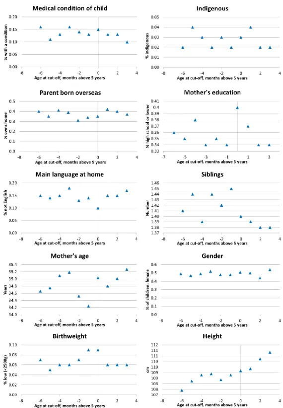
To assess the validity of the instrument exogeneity assumption, we investigate whether there are any discontinuities in selected family and child characteristics at the cut-off in our data. These characteristics include the mother’s education, parent’s country-of-birth, the main language spoken at home, number of siblings, mother’s age, child’s gender, the incidence of the child having a medical condition, indigeneity, birth weight and current height. The results are presented in Figure 2. We find no discontinuities at the cut-off in any of the family and child characteristics. Furthermore, we re-estimated the baseline regression using each of the variables displayed in Figure 2 as the dependent variable. The coefficients on the interaction term (of ESS and FDIS) are not significantly different from zero in all cases except for mother’s age. Thus we tested the sensitivity of our results to the inclusion of mother’s age in the regressions - we find that this did not change our results at all. Last, we test for any discontinuities in the density of children born around the cut-off as proposed by McCrary (2008). Again, we find no discontinuities. We interpret these findings as supporting our identification strategy.
As a further sensitivity test, we re-estimate the model for children whose birth dates are closer to the cut-off. We chose a bandwidth of two months (or two data points) on either side of each state-specific cut-off, following the method suggested by Imbens &
Kalya-9We tried other specifications of age-at-test such as lower order polynomials with the results largely
naraman (2011).10 This is likely to minimise any issues around birth-time manipulation. Here, we also estimate a more general model where we interact the running variable of child age with the indicator for an ill sibling present in the household and allow it to vary by the early school start status. This allows for differential age trends across the children with and without an ill sibling and for early and late school starters. We also exclude age-at-test for this specification. Effectively, our flexible specification means that we are estimating two LATEs - separately for children with and without an ill or disabled sibling. Theγ3k is the difference of these two LATEs. Our results from this general local
model are later presented in Section 7.
A second issue is that of monotonicity (Fiorini, Stevens, Taylor & Edwards 2013). This occurs because the children who are born before the cut-off (and thus eligible to enter school when relatively young) are held back and end up going to school at an even later age than children born after the cut-off. This paper addresses this issue by adopting a binary treatment variable based on whether or not the child was in school at a particular point in time. At this time point, all the compliers are expected to have started school. Children born after the cut-off have not started school, and children who were born before the cut-off but were held back will also not have started school. Thus the latter two groups both take the value of zero for their treatment indicator. In this case, the instrument does not influence the treatment variable in the reverse direction to its intended direction of influence.
5
Results
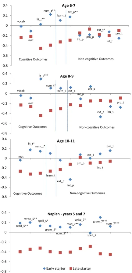
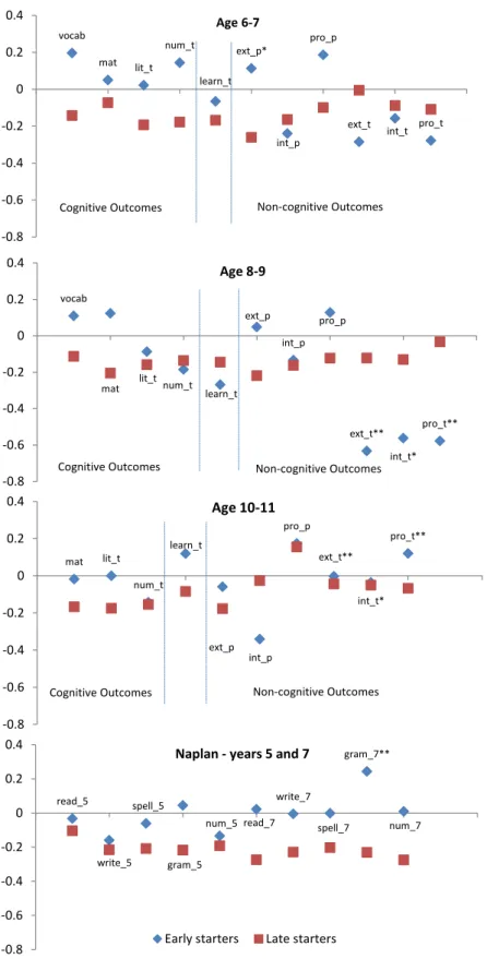
Figure 3 presents the size of the developmental penalty associated with a child having an ill or disabled sibling by the position of the square markers - where the further the square is below the 0-axis the greater is the penalty. These are the estimates for the group of children who start school later and correspond to the coefficient on the poor sibling health (FDIS) indicator in Equation (1). The precise interpretation of the position of each square is the standard deviation difference in test scores, for say the PPVT-vocabulary test, between children who were and were not living with an ill or disabled sibling member at age 4-5 years - and again for the children who start school later. Note that the zero or base category here are those who did not have an ill sibling aand who started school later. Figure 3 shows that the penalty of living with an ill or disabled sibling at that age can be as large as half a standard deviation in test scores - particularly for the NAPLAN cognitive scores.
The penalties associated with having an ill or disabled sibling are pervasive across all our measures of child development. This is indicated in Figure 3 by the squares being consistently below zero along the entire horizontal axis, where we plot the range of devel-opmental indicators. In the top three sub-figures, the indicators range from the cognitive scores for vocabulary, matrix reasoning, and teacher reported information on children’s literacy and numeracy to non-cognitive test scores based on children’s approach to learn-ing and the SDQ scales for externalislearn-ing and internalislearn-ing behaviours and pro-social skills (where we present both parent and teacher responses). These provide three snap-shots of outcome measures when children were aged 6-7, 8-9 and 10-11. In the bottom sub-figure, we plot the test score gaps based on the NAPLAN for reading, writing, spelling, grammar and numeracy for children in the school years of 5 and 7. Across all of these snap-shots, we see a persistent developmental penalty even when children reach the age of 10-11 or when they enter high school (Year 7).11
Our main focus, however, is to understand how the penalties associated with having an ill or disabled sibling vary across children who start school early compared to later. We consistently find that starting school early tends to reduce or even erase the cognitive-based developmental penalties. This is presented in Figure 3 by the position of the diamonds. The level of the diamonds represent the addition of the coefficients on the F DIS indicator and the interaction between the F DIS indicator and the early school start (ESS) indicator in Equation (1). It represents the gaps in developmental scores for children who start school early.
We see that the diamonds hover around (or even above) zero for most of the cognitive test scores thus indicating that starting school early compared to later, tends to reduce (or even erase) the cognitive development penalties associated with having an ill or disabled sibling. The DD estimate is indicated by the distance between the diamond and the square. When the diamond is positioned above the square - this is evidence that starting school early reduces the developmental penalty associated with poor health in the sibling and the greater the height of the diamond relative to the square, the more powerful is the effect of starting school early. We indicate if this DD estimate is statistically significant with the stars where ‘*’ denotes statistical significance at the 10% level, ‘**’ denotes statistical significance at the 5% level, and ‘***’ denotes statistical significance at the 1% level.
11Year 7 is not formally part of high school for the States: South Australia, Queensland, and Western
Australia during the sample period. However, we refer to Year 7 as entering high school as this is accurate for the majority in the states we use.
Figure 3 (bottom sub-figure) shows that starting school early entirely erases the NA-PLAN score penalty associated with having an ill or disabled sibling across all domains of NAPLAN and for both school Years 5 and 7. Note that all students have completed the same number of years of schooling at the time of the NAPLAN tests, regardless of whether or not they are an early or late school starter. These DD estimates (orγ3k’s) are
highly statistically significant. In fact, the diamonds are positioned above the 0-axis, sug-gesting that an early school start more than erases the achievement gaps. However, none of them are statistically significantly different from 0. This is as expected since there is no reason to believe why an early school start would allow children with an ill or disabled sibling to out-perform (in student achievement scores) their relatively advantaged peers who also start school early.12
The impact of starting school earlier in erasing the developmental penalty associated with having an ill or disabled sibling persists even when children complete primary or elementary school. It is clear from the Figure 3 that the early school gains have not diminished by Year 7 NAPLAN scores than they were in Year 5 NAPLAN scores. This increasing gain may reflect the dynamic complementarities in learning and in particular, the benefits of starting this learning process at an early age (Cunha & Heckman 2008). Despite the clear pattern among the cognitive outcomes, starting school earlier has am-biguous impacts on children’s non-cognitive development. Starting school early (mostly) tends to reduce the non-cognitive penalties associated with having an ill or disabled sibling, especially in the shorter term, based on parent-reports. In contrast, it widens children’s developmental penalties in the short term and then narrows the developmental penalties in the longer term based on teacher-reports. This contrast in results when us-ing the parent versus the teacher reports of SDQ scores has also been found in previous research (Becker, Hagenberg, Roessner, Woerner & Rothenberger 2004). It is likely to reflect that these measures capture different information about the child.
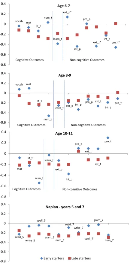
Figures 4 and 5 show that there are also penalties associated with having an ill or disabled mother (Figure 4) or father (Figure 5). These figures also show that starting school early again reduces the magnitude of these penalties. Essentially, we see a similar pattern of effect, albeit somewhat weaker in statistical and substantive significance. Early schooling may play a weaker role in closing the developmental gaps for children with and without an ill or disabled parent for two distinct reasons. First, their parents may have endured the symptoms of the illness or disability for a longer period of time and thus have more experience managing or minimising spill-over effects on the child. Second, parents with
12All the results are tabulated in Appendix Tables A.1 and A.2. Table A.3 then displays the full-set
an illness or disability may have greater availability in time. Both these reasons suggest that the parent’s illness will not compromise the quality of the home environment to the extent that a sibling’s ill health would do so. Indeed, we see that the squares in Figures 4 and 5 are closer to the 0-axis than for those in Figure 3.
6
Explanations for the Narrowing Cognitive Gaps
We now turn to explore why starting school earlier tends to narrow the developmental gaps between children who do and do not have an ill or disabled sibling, compared to starting school later. We focus our analysis on the student achievement (NAPLAN) scores as these results are the strongest.
One hypothesis is that when children receive enough educational stimulation throughout the week, then how they develop is less likely to be influenced by the inputs they receive in the family home. Therefore, the penalty associated with having an ill or disabled sibling at age four-to-five years, for example, will be less for a child who is in school than one who has not yet entered school. We test this hypothesis by regressing the NAPLAN Year 7 outcomes on the same right-hand-side variables as in the main analysis, however, we replace the sibling illness/disability indicator (and its interaction with the starting school early indicator) with a variable that indicates the child was read to frequently (six-to-seven days per week) by a member in the household. We repeat this for other variables such as, the number of siblings in the household, heavy television viewing (three hours or more per day) and parenting style in the form of a measure of ‘warm’ parenting (top third of the distribution based on a survey index construction).13
Here, we aim to test our hypothesis that home inputs matter less when a child is already exposed to a high level of educational stimuli (which is more likely to occur for children who have entered school) - i.e. there are diminishing marginal returns to home inputs. We are not, however, trying to make the link that these home inputs are potential mediating factors in the relationship between the presence of an ill or disabled sibling and weak achievement scores.
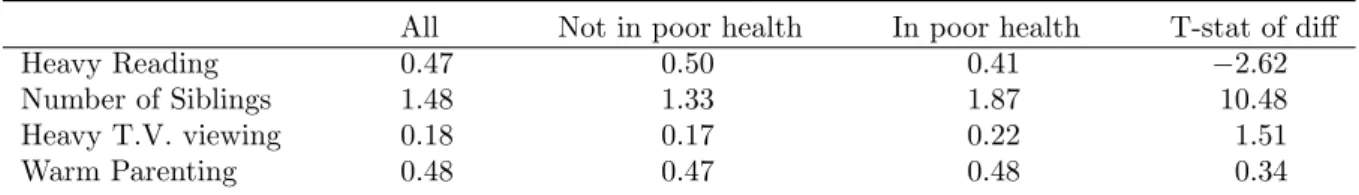
To begin, we show that children who have an ill or disabled sibling tend to receive a lower level of home inputs. Table 2 shows that they are read to less frequently, are more likely to engage in heavy television watching and are more likely to have more siblings than
13We chose these variables because they are correlated with whether or not the study child had a
sibling with an illness or disability at age four to five. They also indicate that the study child is exposed to a home environment that is resource-constrained or low in educational stimulation.
children who do not have an ill or disabled sibling. These differences are only statistically significant at the five percent level for reading frequency and the number of siblings. We see little difference in the level of parental warmth received according to the sibling’s health status.
Table 3 suggests that children’s development is less dependent on the inputs they receive in the family home when children go to school at an earlier age. We see this most strongly for the input of reading on the outcomes of grammar and numeracy. Whereas children who are read to frequently by a household member have much better developmental outcomes than their peers who are read to less often for the children who start school later, this is untrue for children who start school early. For the latter children, their developmental scores are uncorrelated with how often they are read to. We see that the coefficient on the interaction between the early school start variable and the input variable of frequent reading off-set the coefficient on this reading input variable.
A similar story applies to warm parenting and the number of siblings in the household, although the coefficient on the interaction term is not statistically significant for the latter input and weaker in both substantive and statistical significance for the former variable. Surprisingly, we find the opposite effects for heavy T.V. viewing where the negative associations with cognitive outcomes are actually exacerbated for children who enter school early, although not in a statistically significant way. A possible explanation for this is that mothers enter the workforce once their child enters school - a behaviour that is quite common in Australia (Zhu & Bradbury 2015). Thus early school starters may have less access to maternal supervision.
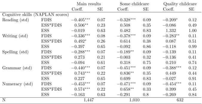
We may expect the benefits of early schooling to be less pronounced when the alternative environment that school is substituting for is already of a high quality. To test this hypothesis, we re-run the analysis for a sub-sample of children who may experience smaller disparities in the quality of the school and home environment, such as those who attended high quality child care while they were young. We expect this group to derive fewer benefits when they enter school earlier because their alternative to going to school may already be educationally enriching. Whereas for children who stay at home or in an environment where the quality of the child care is of lower quality, they may derive greater benefits from starting school at an earlier age.
Previously, we focused on children who were both in high and low quality child care as well as children who did not attend any formal child care before they entered school. Here, we make the following distinctions: children who had some form of non-parent based child care (such as attending a day care centre, family day care, occasional care, a
gym, a leisure or community centre, a mobile care unit, grandparent care, other relative care, nanny care, care by the child’s parent who was living elsewhere, or care by another person (including a friend or neighbour)) and children who used more accredited forms of child care such as centre-based day care, family day care, occasional care, gym, leisure or community centre, and mobile care unit. Note that these types of care arrangements pertain to the child’s first ever care arrangement. Unfortunately, we do not observe the types of care arrangements that all children had in the year preceding school entry. We only observe this for the children who had not yet started school by the time of the wave 1 survey. For the other children, we have information on their first type of care arrangement. However, it appears this variable is highly correlated to the type of care arrangement in the preceding year for those for whom we have this information. For example, 96 per cent of them who said they had some form of non-parent child care for their first child care arrangement were also in non-parent child care in the year before starting school (at age four-to-five).
Table 4 shows that children tend to experience fewer penalties from poor sibling health when they receive high quality child care in their early age. Also, as we expect, these children reap fewer benefits from starting school earlier, in particular for the outcomes of reading and writing. By contrast, children who did not necessarily use high quality child care in their early age (but any form of non-parental care) reaped greater benefits from starting school earlier. Although, the difference in results may be explained by the differences in sample composition i.e. the type of child care that a child attends is likely to be a highly endogenous choice. However, for our purposes, we do not care to disentangle the effects of child care on children’s outcomes from the effect of parental and background factors - we simply use the child care indicator to distinguish between children whose alternative environment is of higher or lower quality.
7
Sensitivity Analysis
In this section, we test how sensitive our results are to variations in the definition and construction of the illness/disability variable. First, we distinguish between the types of illnesses/disabilities that are transitory versus longer-term.14 Second, we consider more exogenous types of family health shocks by controlling for variables capturing the socio-economic and demographic characteristics of the child or his/her family. Third, we
14We also use a non-survey-based indicator of disability in the form of receipt of Carers Allowance - a
Government social assistance payment to carers of children with serious forms of disability. The sample size is significantly smaller, but we still see the story of an early school start narrowing gaps, emerge, albeit in a statistically insignificant way.
re-estimate the results for a restricted sample of children whose birth dates lie within two months of the state-specific cut-off dates.15 In the same regression, we also specify a more general model where we interact the running variable of child age (again, non-parametrically specified as monthly dummy variables) with the indicator for an ill sibling present in the household as well as remove the age-at-test polynomials. Last, we conduct a falsification test to see if we obtain a similar pattern of results in scenarios where we do not expect to see any results i.e. we use a set of cognitive outcome variables that are unlikely to be affected by an early school start.
We find that our results are substantively unchanged regardless of how we define sibling illness/disability. In section 3.2, we outlined how we define a transitory versus a longer-term type of illness or disability. Here, we run separate regressions for them. Table 5 shows three sets of regressions, using three different definitions of sibling illness/disability. The first set of results repeat the main results. The second definition focuses on longer-term types of illnesses or disabilities - those present in siblings across waves 1 and 2. And the third is based on more transitory types of illnesses/disabilities - those present in siblings in wave 1 (and no longer in wave 2). The results are presented for the NAPLAN Year 7 outcomes. Table 5 suggests that even though children are penalised to a greater extent if they were living with a sibling who had a ‘longer-term’ illness or disability as opposed to a ‘transitory’ one at age four to five years, the latter children also endured persistent penalties to their developmental outcomes. We also find that the developmental gaps arising from poor health in the sibling are likely to be off-set whether the sibling had a transitory or a longer-term type of illness or disability but, it is far stronger in the former case.
Turning to the analysis where we examine sibling health shocks that are more exogenous, Table 6 presents the regressions that do and do not control for the social and economic characteristics of the child and his/her family. We control for the following factors: mother’s level of education, whether any parent was born overseas, whether English is spoken in the home, gender of the child, indigenous status of the child, and mother’s age and age-at-birth.16 Note that in our main analysis, where we do not control for these factors, the sibling ill-health variable may be endogenous in the sense that it may have arisen from pre-existing resource constraints in the household. However, we are not concerned with this because we use the sibling ill-health variable simply to indicate whether or not some resource constraint existed in the household during a critical, early stage of the child’s life. Now, by including these family background variables in the
15We also tried other bin lengths such as one and three months. The results are substantively similar.
16We also run a separate regression, restricting the sample to only children with siblings and we find
regression, we will minimise any effect they may have through the incidence of sibling ill-health, as well as possibly controlling away legitimate channels of the sibling health effect. Table 6 suggests that going to school early is also very effective in reducing the developmental gap between children who do and do not experience a sibling ill-health shock i.e. those that are (largely) independent of family background.
In Table 7, we show our results to be largely insensitive to model specification and to the bin-width around the cut-off threshold. In this regression, we simultaneously perform a number of changes to the model. First, we restrict the sample to children whose birth dates are two months on either side of the cut-off date; second, we specify the most general model by interacting the running variable of child age (again, non-parametrically specified as monthly dummy variables) with the indicator for whether an ill sibling is present in the household; and third, we remove the age-at-test polynomials. This model represents our most general and non-parametric specification.17 As we use a bin width of two months on either side of the state-specific cut-off dates, the sample size reduces to approximately 500 child observations. Despite the reduction in sample size, we find the results are largely consistent with the main results, albeit weaker in statistical significance. Table 7 shows that an early school start continues to off-set the negative effects of the presence of an ill sibling in the household in all cases except for reading. We also can draw broadly similar conclusions from the coefficients on the sibling disability and the early school start indicators.
Last, we conduct a falsification test where we repeat the same exercise for cognitive outcomes that are unlikely to have been affected (yet) by early school entry. Specifically, we use outcomes that were measured at wave 1 when children were aged four-to-five years such as, the Peabody (PPVT) vocabulary test, Who Am I (WAI), Reading, Writing and Numeracy competency tests. At the time they were surveyed, the children who had started school had only been in school for one-to-three months. We expect this is too short a time for any effect of schooling to be realised in (cognitive) test scores.
Table 8 contrasts the results using comparable measures at age four-to-five and at age six-to-seven. The same set of right-hand-side variables appear in these two sets of results. The outcome measures used at age four-to-five include interviewer generated test scores for vocabulary (PPVT) and a measure of IQ (Who Am I, WAI) as well as teacher gener-ated scores of reading, writing and numeracy competency. The comparable measures at age six-to-seven include again, vocabulary (PPVT), matrix reasoning, and teacher-rated scores of literacy and numeracy. All these scores, as per the main analysis, have been
17The results are substantively similar when we introduce these distinct sensitivity test steps gradually