INTERACTIVE PHYSICALLY-BASED CLOUD SIMULATION

INTERACTIVE PHYSICALLY-BASED CLOUD SIMULATION

A Thesis by

DEREK ROBERT OVERBY

Submitted to the Office of Graduate Studies of Texas A&M University

in partial fulfillment of the requirements for the degree of MASTER OF SCIENCE

May 2002

A Thesis by

DEREK ROBERT OVERBY

Submitted to Texas A&M University in partial fulfillment of the requirements

for the degree of

MASTER OF SCIENCE

Approved as to style and content by:

John Keyser (Chair of Committee) Bart Childs (Member) Ergun Akleman (Member) Jennifer Welch (Head of Department) May 2002

ABSTRACT

Interactive Physically-Based Cloud Simulation. (May 2002) Derek Robert Overby, B.S., Texas A&M University

Chair of Advisory Committee: Dr. John Keyser

Clouds play an important role in the depiction of many natural outdoor scenes. Realistic modeling and rendering of such scenes is important for applications in games, military training simulations, flight simulations, and even in the creation of digital artistic media. Previous methods for modeling the growth of clouds do not account for the fluid interactions that are responsible for cloud formation in the physical atmosphere. We propose a model for simulating cloud formation based on a basic computational fluid solver. This allows us to simulate the complex air motion that contributes to cloud formation in our atmosphere. Among the natural processes that we simulate are

buoyancy, relative humidity, and condensation. Because we have built this model on top of a visually realistic fluid simulator with which the user is able to interact, we are also able to give the user artistic control over a physically accurate environment.

In practice, the user need only set the initial conditions for our virtual atmosphere to produce different types of cloud formations.

ACKNOWLEDGEMENTS

I would like to thank everyone who has contributed to this project, especially my colleague and partner in research, Zeki Melek, who has been around to help answer countless questions. I would also like to thank my advisor, John Keyser, for guiding my vision and helping me to get my work published. I must also thank Dr. Mike Biggerstaff of the Texas A&M Meteorology Department, Mark Harris of the University of North Carolina for his ongoing help with rendering, and my brother Darryl for his help with the fluid dynamics. I thank my parents for giving me the education and discipline to

complete this project, as well as all the teachers, professors, and authors whose words and instruction have given me the opportunity to learn how to learn and think for myself. And finally I must offer the greatest thanks and appreciation to my soul mate, Kristie, without whose love and support I could not have done any of this.

TABLE OF CONTENTS

LIST OF FIGURES……… viii

1 INTRODUCTION……….. 1

2 PREVIOUS WORK……… 3

2.1 Cloud Models in Computer Graphics……….. 3

2.2 Cloud Models in Meteorology………….……… 20

3 CLOUD FORMATION IN THE ATMOSPHERE……… 22

3.1 Thermodynamics………. 24

3.2 Physical Process……….. 25

4 FLUID MODEL………. 32

4.1 Fluid Model Basics………. 32

4.2 Application of Fluid Model to Atmospheric Simulation…... 36

5 CLOUD MODEL………..……… 38

5.1 Software Model……….. 38

5.2 Interface………..……… 43

5.3 Creating Different Cloud Types……….. 46

6 RESULTS AND PROBLEMS ENCOUNTERED………. … 50

7 IMPLEMENTATION DETAILS……… 53

7.1 Data Structure……….. 53

7.2 Visualization……… 54

Page 7.4 Constraints………... 55 8 FUTURE WORK……… 56 9 CONCLUSIONS……… 59 REFERENCES……… 60 APPENDIX A……… 63 APPENDIX B……… 64 APPENDIX C……… 65 APPENDIX D……… 66 APPENDIX E……… 67 VITA ……… 68

LIST OF FIGURES

FIGURE Page

1 Kajiya example………... 5

2 Example of Perlin noise, courtesy of Zeki Melek ……….. 5

3 Example of clouds using Lewis method………. 6

4 Transition functions for Nagel’s cellular automaton……….. 7

5 Clouds generated using Nagel’s method……… 7

6 Example of Neyret’s clouds………. 8

7 Convection simulated using CML………. 9

8 Miyazaki example……….. 9

9 Blinn’s volume rendering method………. 11

10 Example of Gardner’s textured ellipsoids………. 12

11 Max example………. 13

12 Levoy example………... 14

13 Concentric spheres used in Dobashi method………. 15

14 Visual description of Dobashi method……….. 15

15 Image from Dobashi method………. 16

16 Example of Harris’s rendering method………. 16

17 Particle system proposed by Reeves in 1983……… 18

18 Foster and Metaxas example………. 19

FIGURE Page

20 Air-Mass Thunderstorm………..… 21

21 Cumulus cloud formation……… 22

22 Stratus cloud formation………... 23

23 Artificial cloud seeding over 45 minute period………... 26

24 Example of ascension caused by convection……….. 27

25 A cloud formation caused by orographic uplift……….. 28

26 Graph of pressure vs. altitude……… 29

27 Visual depiction of cloud droplet size……… 30

28 Continuous collision model……… 31

29 Backward tracing time-step method proposed by Stam………. 36

30 Heat enters the environment from defined sources at ground level… 40

31 Humidity is shown being advected upward by thermal currents…... 40

32 Graphical User Interface for cloud modeling application ………… 43

33 Wind interface……… 45

34 Source interface………. 45

35 Cumulus cloud formation caused by vertical air movement………. 47

36 Stratus cloud formation caused by horizontal air flow………. 48

37 Proposed expansion algorithm in two dimensions..……….. 51

38 Proposed momentum conservation algorithm………... 52

39 Simulation pipeline……… 55

FIGURE Page 41 Second view of clouds generated and rendered using Dobashi

method……….. 63

42 Humidity field being advected by buoyancy……… 64

43 Heat field……….. 64

44 Resulting cloud field……… . 64

45 Graph of pressure vs. altitude in the troposphere.……… 66

1 INTRODUCTION

The digital creation of clouds is important for many applications in Computer Graphics, including those involving the rendering of outdoor scenes. Fast, efficient methods of generating clouds are valuable tools for these and other applications such as outdoor simulations and the digital rendering of atmospheric effects. These models are used extensively by both the motion picture industry and the gaming industry, often as background imagery. By making the background content of outdoor images appear more natural, the graphic artist can more skillfully direct the viewer's attention. The modeling of realistic cloud shape is fundamental for the creation of these types of digital images. In this paper, we focus on the simulation of physical processes that contribute to the formation of clouds in our lower atmosphere1. By simulating these physical

processes we are able to more accurately model the structure of a cloud that forms under given atmospheric conditions.

Previous methods for generating cloud models have traditionally used a procedural or fractal method to generate cloud structure [Nagel and Raschke 1992]. While these methods may at times produce visually compelling results when coupled with complex rendering

This thesis follows the style and format of ACM Transactions on Graphics.

1 _{In this paper, when we refer to the atmosphere, we are referring specifically to the troposphere or sphere}

of weather [Wallen 1992]. The troposphere is the lowest division of our atmosphere which extends from the ground to an altitude of approximately 12km.

techniques, these structures are essentially deterministic and are difficult to modify for creating different cloud types. Our method allows the user to interact in with a

physically-based simulated environment in order to produce the desired cloud formation. All the user needs is a basic understanding of the fundamental processes involved in cloud formation: buoyancy, relative humidity, and condensation. By manipulating the parameters of these processes in our simulation, the user is able to interact with the simulation.

First we will discuss previous work on this topic both in the field of Computer Science and also in the field of Meteorology. We will then discuss the physical process of cloud formation in our atmosphere in Section 3. In Section 4 we will discuss the fluid model upon which our simulation is based. In Section 5 we present our proposed

software model for the physical process of cloud formation, and in Section 6 we discuss results and problems that were encountered during the course of this research. We will discuss various details of our implementation in Section 7. In Section 8 we present several directions for future work, and finally we present our conclusions in Section 9.

2 PREVIOUS WORK

Cloud modeling has been a subject of extensive research in both Computer Science and Meteorology. Both fields have been active in researching methods for simulating, visualizing, and predicting clouds and other natural phenomena that occur in our atmosphere.

In section 2.1 we discuss previous models of cloud formation in the field of Computer Graphics and some of the advantages and shortcomings of these methods. This section is divided into three categories, corresponding to three main categories of cloud models that have been studied. Procedural models are discussed in section 2.1.1, rendering models in section 2.1.2, and particle systems and fluid models in section 2.1.3. Then in section 2.2 we present a brief look at some models of cloud formation in Meteorology and why they are so different from those in Computer Graphics.

2.1 CLOUD MODELS IN COMPUTER GRAPHICS

Within the field of Computer Graphics there has been extensive research aimed at quickly generating realistic looking clouds. Early research was hindered not only by the large memory and processing requirements inherent when working on and rendering volumetric data on a coarse grid, but also by the limited rasterization functions provided

by the contemporary graphics hardware. However, realistic fluid motion can now be obtained on coarse grids through the use of recently proposed efficient three-dimensional fluid solvers [Stam 1999]. Also, the memory and processing power provided by today's desktop PC's has greatly improved our ability to simulate complex interactions like fluid motion.

2.1.1 PROCEDURAL MODELS IN COMPUTER GRAPHICS

In 1984, James Kajiya presented his paper in which he not only presented methods for single and multiple scattering2, but also presented a method for modeling the formation of cloud structure based on atmospheric fluid dynamics [Kajiya and Von Herzen 1984]. However, in his method Kajiya accounted for the effects of viscosity, as well as using a less accurate method for simulating the fluid motion in the system. An example of clouds produced by Kajiya using this method are shown below in Figure 1.

2_{Single scattering refers to a reflectance model which only accounts for one reflection of light from a light}

source, while multiple scattering refers to a reflectance model in which more than one reflection is considered.

Figure 1: Kajiya example. Figure taken from [Kajiya and Von Herzen 1984].

Many early implementations of cloud models were based on the work presented by Perlin [1989] in which he presented a method for generating continuous random data within a volumetric space. The method was based on using harmonics, or series of overlapping waves, to generate a continuous function. An example of Perlin noise is shown below in Figure 2.

Contemporary work by Lewis [1989] was also based on using random functions to approximate clouds, but his method used two dimensional random textures applied to ellipsoids to make his clouds. The textures also included opacity values, to give the clouds some transparency. An example of Lewis’s method is shown in Figure 3.

Figure 3: Example of clouds using Lewis method. Figure taken from [Lewis 1989]

Other early models of cloud structure were developed within the field of

Mathematics. In their 1992 paper, Nagel and Raschke [1992] presented a model of cloud growth based on a simple Boolean function iterated within a volumetric data space. This method, which is called a cellular automaton and shown in Figure 4, can give a somewhat realistic looking growth pattern for the formation of a cloud. However clouds that are generated using this method are limited to growth in one direction and

tend to produce very uniform cloud structures. An example of clouds generated using this method is shown in Figure 5.

Figure 4: Transition functions for Nagel's cellular automaton. Figure taken from [Dobashi et al. 2000]. Act, hum, and cld are the three fields which are updated by the transitions functions.

Another model which was presented by Fabrice Neyret in 1997 is based on simulating high-level process such as currents, vortices, and bubbles to produce a simulation of cloud formation. This model is quite unique in its focus on these high-level phenomena that occur in the atmosphere and their contributions to cloud formation [Neyret 1997]. An example of clouds generated using Neyret’s method is shown in Figure 6. The use of bubble-like particles is evident in this image.

Figure 6: Example of Neyret's clouds. Figure taken from [Neyret 1997].

In 1990, Kaneko presented a method for simulating physical processes with an expanded version of the cellular automaton used in Nagel’s method. He used a Coupled Map Lattice to simulate convection currents in two dimensions. Since that time, this work has been used to simulate many other physical processes, especially gaseous phenomena. An example of 2D convection generated using CML is shown in Figure 7.

Figure 7: Convection simulated using CML. Figure taken from [Miyazaki 2001].

Recently, Kaneko’s method has been applied to generating clouds based on

atmospheric fluid dynamics in a paper by Miyazaki et al. [2001]. This method, used in conjunction with Dobashi’s rendering methods, can produce excellent results of cirrus cloud formations as shown below in Figure 8.

The problem with procedural methods is that in the quest to mimic the seemingly random shape of natural clouds, they can quickly become gross mathematical

abstractions of simple fluid motion. Furthermore, these methods are not based on the many physical processes which contribute to natural cloud formation in our atmosphere.

2.1.2 RENDERING MODELS IN COMPUTER GRAPHICS

Computer rendered clouds are often generated for the purpose of background

imagery, and therefore the primary goal of the modeler is to fool the eye into dismissing the puffy thing it sees in the background as a cloud. By making the cloud appear more natural in color and texture, the artist can draw the viewer's eye away from the actual structure of the cloud and toward the heart of the image. Such effects can be achieved using only rendering techniques and artistic control, without actually putting much effort into the underlying model of the cloud. Our model differs in that we seek to create an accurate model of the growth of the cloud's volumetric structure. Any of these advanced rendering methods can be used with our data to produce excellent offline images or animations of cloud formation.

Some of the earliest work on volume rendering was presented at SIGGRAPH by Jim Blinn in 1982. Blinn’s method was the first to address the light interactions that occur

when light passes through a low-albedo3 particle cloud. An image taken from Blinn’s paper is shown in Figure 9.

Figure 9: Blinn's volume rendering method. Figure taken from [Blinn 1982].

Another early rendering concept was presented in 1985 by Gardner. Gardner’s idea was to create a cloud scene using both 2D and 3D representations. He would use a two dimensional texture to display high-level clouds in the background, while using 3D textured ellipsoids to model foreground clouds. An example of a scene generated by Gardner using this method is shown below in Figure 10.

3_{Albedo refers to the reflectance ratio of the material. Therefore a low-albedo analysis accounts more for}

Figure 10: Example of Gardner's textured ellipsoids. Figure taken from [Gardner 1985].

Work in 1986 presented by Nelson Max also contributed to the art of rendering volumetric data. Max presented a method for rendering atmospheric effects such as shadows and attenuation based on a scanline algorithm implemented in polar

coordinates. This method is also applicable to rendering clouds and other volumetric data where atmospheric effects are desired. An example of Max’s work is shown in Figure 11.

Figure 11: Max example. Figure taken from [Max 1986].

As the rendering of volumetric data was more fully explored by researchers, the field of medicine supplied a practical application for these methods, as well as a new source of high-resolution data. Medical diagnosis procedures such as MRI and CT4 scans produce very high-resolution data sets, which must be visualized in order to be useful for doctors and surgeons. In 1990 Marc Levoy presented an efficient method for volume rendering that made use of octree data representations and adaptive termination of rays. An example of a rendering using Levoy’s method is shown in Figure 12.

Figure 12: Levoy example. Figure taken from [Levoy 1990].

Much of the recent research into advanced rendering methods for clouds and other volumetric data has focused on accounting for effects such as skylight and atmospheric attenuation5_{. Yoshinori Dobashi has presented an efficient method for rendering}

volumetric cloud data in which several transparent concentric spheres are rendered in front of the viewer [Dobashi et al. 2000], as shown in Figure 13. The texture that is mapped onto these spheres is a function of atmospheric attenuation at each vertex. This gives very nice renderings of sunsets and other scenes in which sunlight shines through from behind the clouds. A visual description of Dobashi’s rendering method is shown in Figure 14, and an example of Dobashi’s method is shown in Figure 15.

5_{Atmospheric attenuation is responsible for shafts of light protruding through large cloud formations. It is}

Figure 13: Concentric spheres used in Dobashi method. These spheres are mapped with a texture which is a function of atmospheric attenuation and then rendered around the viewpoint so that the

viewer looks through them.

Figure 14: Visual description of Dobashi method. Image taken from [Dobashi et al. 2000]. Shows how vertex computations are used to create shafts of light.

Figure 15: Image from Dobashi method. Image taken from [Dobashi et al. 2000].

Recent research into rendering methods includes that by Harris and Lastra [2001]. Their paper focuses on using imposters to speed up rendering, approximating multiple forward and anisotropic scattering of light through volumetric data. An example of Harris’s work is shown in Figure 16.

2.1.3 PARTICLE SYSTEMS AND FLUID MODELS IN COMPUTER GRAPHICS Other methods have developed models in Computer Graphics by making use of techniques designed to approximate fluid motion. Traditionally, many of these models have been based on particle systems, but methods have also been implemented using both regular and irregular grid structures.

Some of the earliest work presented regarding using particle systems for modeling fuzzy objects was presented by William Reeves in 1983. Reeves presented a technique for using a particle system to model fire, clouds, or water. He did this simply by

designing the particles' behavior to mimic the desired fluid motion [Reeves 1983]. This work was introduced to the motion picture industry in the movie Star Trek II: The Wrath of Kahn, and is shown in Figure 17.

Figure 17: Particle system proposed by Reeves in 1983. Figure taken from [Reeves 1983].

Others have developed methods which use the principles of physics and fluid

dynamics to model the motion of fluids for computer models. Early CG research in this area was presented by Foster and Metaxas [1997], whose model was one of the first in the field of Computer Graphics to be based on the Navier-Stokes solution. An example of the Foster and Metaxas model of fluid flow is shown in Figure 18. Fedkiw and Stam have recently presented a method for efficiently modeling the fluid-like motion of a substance such as smoke [Fedkiw et al. 2001], while Fedkiw and Foster have developed models of different fluids such water and mud [Foster and Fedkiw 2001]. An example of the more recent method presented by Fedkiw and Stam is shown in Figure 19. Details of this method will be discussed in more detail in section 4.

Figure 18: Foster and Metaxas example. Figure taken from [Foster and Metaxas 1997].

2.2 CLOUD MODELS IN METEOROLOGY

There is a fundamental difference in the approach that the meteorologist takes when modeling clouds from the approach that the computer scientist takes. The Computer Graphics perspective is to strive primarily for visual effect and speed. The goal is to simulate as little as necessary to get the desired level of detail. On the other hand, the meteorologist will try to get the highest level of accuracy possible, regardless of how long it takes or how it looks. The meteorological approach to modeling nature is to simulate everything that physics can tell us, and thus these models are inherently different than models developed within the field of Computer Graphics.

To understand the meteorological approach, we must first examine the way in which meteorologists have traditionally studied the atmosphere. Extensive, documented research into storm systems began as early as the 1940's when commercial aviation began to first feel the threat of severe weather. After WWII, Congress decided to make use of some of the Air Force's Northrup P-61C-type airplanes [Braham 1996], in order to gain a better understanding of how weather patterns formed thunderstorms. This project, known as the Thunderstorm Project, has been the largest study to date of storm

formation. It used a multitude of sensors both on the ground and in the air for many large storm systems. A total of 76 thunderstorms were recorded [Braham 1996]. From this study, Byers and Braham developed a model thunderstorm formation called the Air-Mass Thunderstorm, shown in Figure 20. The model was a three-stage model of storm

development: the cumulus stage, the mature stage, and the downdraft stage. This study was only the beginning of this area of research in meteorology, however the dataset from this project remains one of the largest of storm data to this day, and is still used as input for many contemporary meteorological models.

Figure 20: Air-Mass Thunderstorm [Byers and Braham 1949].

Today research in this area has culminated in a distributed project called Mesoscale and Microscale Meteorology. The MMM simulator is able to simulate almost all known atmospheric phenomena on both meso- and micro- scales. Simulations can take anywhere from days to minutes, depending on the resolution and the amount of detail required. More information on the MMM Project can be obtained from the National Center for Atmospheric Research6 or Pennsylvania State University7.

6 _{MMM Home Page, National Center for Atmospheric Research.}

http://www.mmm.ucar.edu/mmm/home.html

3 CLOUD FORMATION IN THE ATMOSPHERE

The study of clouds has never been limited to scientists alone. Artists, poets, and even daydreamers watch with interest as the clouds constantly change before their eyes. At any one time, nearly half of the earth's surface may be obscured by cloud cover [Wallace and Hobbs 1977]. This is because there are so many different ways for cloud to form in our atmosphere. Two of the most common types of clouds are convective clouds and layer clouds. Convective clouds are formed by the local ascent of warm air parcels in a conditionally unstable environment [Wallace and Hobbs 1977]. Convective clouds are also known as cumulus clouds and can be distinguished by their

predominantly upward growth. These clouds range in size from 0.1 to 10 km. Their ascension velocities can range anywhere from 1 m/s to 10 m/s, and they can last from minutes to hours [Wallace and Hobbs 1977]. An example of a cumulus cloud formation is shown in Figure 21.

Layer clouds, on the other hand, which are also known as stratus clouds, are

produced by upward motion of stable air and may occur anywhere from ground level up to the tropopause8. These clouds can extend from hundreds to thousands of square kilometers, are usually driven by vertical velocities ranging from 1 to 10 cm/s, and can last for tens of hours [Wallace and Hobbs 1977]. An example of a stratus cloud formation is shown in Figure 22.

Figure 22: Stratus cloud formation. Figure taken from [Wallen 1992].

In addition to cumulus and stratus clouds, clouds can also be classified as either cirrus or nimbus. Cirrus clouds are those clouds which appear fibrous, and nimbus refers to any cloud that precipitates. Most clouds can be classified by one of these types or their compounds, like cirrocumulus or cumulonimbus. Of course there are many more

documented cloud types than we will present here. However, for those interested more information can be found in the International Cloud Atlas, published by the World Meteorological Organization in 1956.

3.1 THERMODYNAMICS

Several thermodynamic principles are active participants in the formation of clouds in our atmosphere. One of the foremost and most relevant for our simulation model is the ideal gas law, given in Equation 1.

nRT PV =

Equation 1. P is pressure, V is volume, n is number of moles, R is the universal gas constant9_{, and T}

is temperature.

This equation tells us that, given constant pressure in a gas under ideal conditions, volume and temperature will be directly proportional. Or, given constant volume, the pressure and temperature will be directly proportional. Because of this relationship, a rising parcel of air will experience a decrease in temperature just as it experiences a decrease in pressure10. 9 _{Given as} K mol J ⋅ 315 . 8 [Lide 1992].

3.2 PHYSICAL PROCESS

3.2.1 STAGE ONE: DIRTY MOIST AIR

The physical process of cloud formation as it occurs every day in our atmosphere is a quite complicated process. In order for the process to begin, the presence of “dirty moist air” is required. We must have air which contains tiny particles, called hygroscopic nuclei, upon which the water vapor can condense11, along with having air saturated with water vapor (near 100% relative humidity12). Water vapor can actually condense at relative humidity levels lower than 100% if the air contains a high concentration of these particles (over 50%). For example, in a city with severe air pollution clouds may form with relative humidity as low as 76% [Wallen 1992]. Also, cloud formation can be artificially aided by increasing the local concentration of hygroscopic nuclei. In fact, this is the same concept used in artificially seeding real clouds — planes release fine particles into saturated air to aid in the condensation process [Wallen 1992]. An example of this is shown in Figure 23.

11 _{In order to condense, pure water must have a surface to adhere to.}

12_{Relative humidity is the amount of water within a differential volume of air over the total amount of}

water vapor that differential volume can hold (which is dependant upon pressure and temperature) [Wallen 1992].

Figure 23: Artificial cloud seeding over 45 minute period. Figure taken from [Wallace and Hobbs 1977].

3.2.2 STAGE TWO: ASCENSION

The second stage in atmospheric cloud formation is ascending air. Ascension is most often caused in our atmosphere by thermal currents. Thermal currents are the result of buoyancy within our atmosphere. The surface of the earth, warmed by the sun, radiates heat into the atmosphere, which causes the temperature of the air to increase. This causes the air to expand due to increased local pressure and then rise due to buoyancy13_.

13 _{Buoyancy is a result of variation in density within a fluid. In our simulation, we do not account for local}

A visual example of how temperature variations create thermal currents is shown in Figure 24.

Figure 24: Example of ascension caused by convection. Figure taken from [Wallen 1992].

Ascension of air can also be caused by orographic uplift which is when air is ‘pushed up’ by the terrain below it. For example, clouds often form around mountain ranges as the air blows up and over the surface of the mountain [Wallen 1992]. An example of this is shown in Figure 25.

Figure 25: A cloud formation caused by orographic uplift. Figure taken from [Wallace and Hobbs 1977].

3.2.3 ADIABATIC COOLING/SATURATION

As air rises, pushed by either buoyancy within the air or orographic uplift, the air expands as the pressure decreases. The decrease in pressure results in a proportional decrease in temperature. A graph of pressure (mBar) vs. altitude (km) is shown in Figure 26. Because cool air is able to hold less water vapor than warm air, the result is an increase in relative humidity as a moist air parcel rises. Eventually, the rising air will reach a point of saturation. The temperature at which this occurs is called the dew point.

Figure 26: Graph of pressure vs. altitude. Data taken from [Lide 1992].

3.2.4 CONDENSATION AND LATENT HEAT

Once the dew point has been reached and if hygroscopic nuclei are present,

condensation will occur. Since the process of condensation is an exothermic process, it causes the release of what is called the latent heat of condensation. This energy, which is proportional to 2.5×106 Jkg[Wallace and Hobbs 1977], increases the temperature of the nearby air, thus increasing it's buoyancy and causing the air to rise even more. This is why so many clouds seem to grow upward, especially when the surrounding air is calm. Different atmospheric conditions contribute to the growth of different cloud types, which will be discussed later in section 5.3.

3.2.5 PRECIPITATION

The final stage of the process is precipitation. Precipitation is a gradual process involving the collision and coalescence of condensed cloud droplets. As droplets collide with each other within the cloud, many smaller droplets will combine to create a few larger droplets. As these droplets grow in mass, the gravitational force exerted upon them increases and thus the terminal velocity of these droplets increases. This increase in size and velocity also increases the probability of collision. Figure 27 below shows a comparison in size among cloud droplets and their larger counterparts, raindrops. CCN stands for Cloud Condensation Nuclei, and is equivalent to our concept of hygroscopic nuclei. In the figure, r is the radius in micrometers, n is the number of particles per liter of air, and v is the terminal velocity in cm/s.

Figure 27: Visual depiction of cloud droplet size. Figure taken from [Wallace and Hobbs 1977].

The statistical model of the precipitation process is called the continuous

of droplet size within a cloud based on a stepwise function of collision probability. The collision probability in the figure is ₁₀1 _{. One shortcoming of this model is that it fails to} consider increased probability associated with increasing size, although it can be argued that such a small change in size may not affect collision probability. As a point of fact, however, the complete collision probability solution is much more complicated,

involving not only accurate simulation of simple physical properties of cloud droplets such as mass, velocity, and acceleration, but also more complicated characteristics such as surface tension and body deformation. However, for the purposes of a visual

simulation, this model would present an adequate basis for a simulated model of the precipitation process.

4 FLUID MODEL

Our simulation of cloud formation is based upon an implementation of a course grid fluid solver presented recently by Stam [1999]. This solver uses the Navier-Stokes fluid equations to model fluid flow through a volumetric space. Here we present a brief description of the Navier-Stokes solution and why it is acceptable for our model. For details concerning our implementation, the reader should consult both Stam's paper [1999] and the paper by Fedkiw et al [2001].

4.1 FLUID MODEL BASICS

The Navier-Stokes solution is an approximation of incompressible flow.

Incompressible flow is that which contains no sharp changes in density, as would be caused by a supersonic shockwave. This model is preferred to those of compressible flow because compressible flow solutions require relatively small time steps to maintain accuracy. There is no disadvantage to using incompressible flow as long as the

maximum flow speed remains below Mach 1 (the speed of sound) [Brower 1999].

When building a model of fluid flow, we begin by assuming that mass is conserved. This means that the net change in mass must always be zero. This is expressed

change in density

(

)

t

u

=

−

⋅

∇

_ρ

Equation 2

In Equation 2, ρ is the density and u is the vector field representing velocity within the fluid. If we assume that our density is constant (∂_∂ρ_t

=

0

0

=

⋅

∇

u

Equation 3

This equation expresses conservation of mass within our system, and is required for the system to be properly constrained. We need four equations to solve for the four unknowns in a fluid system: velocity in x,y,z directions and pressure. Therefore

Equation 3 and the three Navier-Stokes equations are a complete solution for fluid flow. The Navier-Stokes equations can be written together as shown below in Equation 4 [White 1991].

ρ ρp

ν

₊

_u

_⋅

_∇

_u

₌

₊

_∇

_u

₊

₍

₎

The terms on the left of the equation are our inertial acceleration terms. The first term expresses our temporal acceleration while the second expresses spatial effects within the system. On the right of the equation we have a pressure term followed by a term which expresses the viscous force (shear stress). The final term, f, represents any external forces per unit volume applied to the system. This equation shows that motion within the system is dependant upon force due to pressure, force due to viscous effects, and force due to any external forces such as gravity (or buoyancy).

Because the inertial effects outweigh the contribution of viscous effects in air, we can ignore the viscous term. To see this we examine the Reynolds number for our system. The Reynolds number expresses the dimensionless ratio of inertial forces to viscous forces and is given below in Equation 5 [White 1991]:

νL

u

R

₌

In Equation 5 u is a characteristic velocity, L is characteristic length and ν is kinematic viscosity14. For air at approximately 20 °C, m s

2 5 10 4 . 1 × − = ν [Lide 1992].

Also, since the troposphere extends approximately 12 km from the surface of the earth [Wallen 1992], we can use ₁₀3m _{as our characteristic length. Therefore, in order for the} Reynolds number to be 1.0 (where the inertial effect equals that of the viscous effect), our flow speed would have to remain below 10−8ms. Since the fluid motion we will be modeling will be much faster than this, we can assume that R>>1 and therefore viscous effects can be ignored. Although the precise value of the characteristic length (L) or kinematic viscosity )(ν may vary slightly in a particular simulation, this remains a safe assumption since the Reynolds number will remain much greater than 1. Looking at the Navier-Stokes equation again, we can see that, having removed the viscous term, our inertial acceleration in the system will be balanced by pressure and external forces within the system. This makes our fluid flow computation much easier since we do not have to compute the effects of viscosity.

The fluid solver we use for our simulation, presented by Stam [Stam 1999], is based on this Navier-Stokes system. At each simulation step, the Navier-Stokes equations — neglecting the viscous term — are solved for each voxel in the grid. One of the main aspects of this method is the use of backward-tracing particle motion within the system. This approach allows for unconditional stability even when using large time steps and is

14 _{The kinematic viscosity of a material is defined as the fluidic viscosity of the material over the density}

shown in Figure 29. As shown in the figure below, at each timestep we trace the motion of a particle in the direction of it’s current velocity times −∆t. Instead of calculating where a particle is going, we are calculating what is coming toward this particle. This method introduces a small amount of inaccuracy, but makes the simulation much more stable and allows for larger timesteps.

Figure 29: Backward tracing time-step method proposed by Stam. Figure taken from [Stam 1999].

4.2 APPLICATION OF FLUID MODEL TO ATMOSPHERIC SIMULATION

In order to apply this fluid model to a simulation of the atmosphere, we must account for several discrepancies between the model and the actual atmosphere. As we have mentioned previously, the Navier-Stokes model of fluid motion assumes constant

pressure and density of air, which is not realistic in the atmosphere. Air in our atmosphere is stratified, meaning that its pressure and density decrease as we go up. Fortunately for us, these variances in pressure and density do not affect the motion of the fluid within the atmosphere, since the only direct affect of these changes would have on fluid motion would be realized as effects of viscosity (in our model viscous effects are ignored). What these changes in pressure and density do affect are the processes that occur at different altitudes within our simulation. For example, the pressure and density of air does have an effect on the amount of water vapor the air can hold, which directly affects the relative humidity computation in the simulation. Therefore, although we do not model local changes in pressure or density of the air, we do keep track of these values and how they change over large changes in altitude. By storing pressure and density values in lookup tables, we are able to use empirical data from the atmosphere to compute derived values such as relative humidity and how they change with varying altitude.

5 CLOUD MODEL

In this section we discuss our software model of the physical process of cloud formation in the atmosphere. In section 5.1 we present the software model we have developed to mimic this physical process. In section 5.2 we briefly discuss the user interface we have developed and in section 5.3 we describe how we can use our software model and interface to produce different types of clouds. Pseudocode for the software model is included in Appendix C.

5.1 SOFTWARE MODEL

We have mentioned that our model of cloud formation is physically based. What this means is that we simulate the condensation of water vapor within the atmosphere based on parameters derived from the physical process. To do this we must model the fluid flow of air in our atmosphere. Local airflow is based on a number of environmental factors, including large-scale wind and turbulence.

Aside from modeling the local motion of the air, we must also model the thermal currents that occur in the atmosphere. We do this by modeling the motion of heat energy in the atmosphere. We first define heat sources at ground level. These sources radiate heat into the atmosphere. We are able to compute the temperature of any point in the

field by multiplying the amount of heat energy present by the pressure, as shown in Equation 6. The pressure in our system is defined as a gradient based on altitude. The pressure is 1.0 Bar at ground level and decreases exponentially with height to 0.1 Bar at the tropopause15. These values are taken directly from measurements within our own atmosphere [Wallen 1992].

local local

local

E

P

T

=

×

Equation 6: Temperature computation. T_local is temperature, E_local is heat energy, and P_local is pressure.

Once we compute the temperature at each point we use this information to compute our buoyant forces. At each point, if the surrounding temperature16 is less than the current temperature at that point then we add a positive buoyant force. Likewise, if the surrounding temperature is greater than the current temperature, we add a negative buoyant force. This enables us to model the thermal currents in our atmosphere caused by heat sources. We compute the actual buoyant force added to our system as shown in Equation 7, where K_buoyancy is a user-defined constant. Figure 30 shows heat being added to the system and causing buoyancy, and Figure 31 shows humidity within the system being advected upward by that buoyant force.

15 _{The tropopause refers to the upper boundary of the troposphere.}

16 _{The surrounding temperature is computed by averaging the temperature values for all neighbor voxels in}

)

(

buoyancy

buoyancy

K

T

T

F

=

−

Equation 7: Buoyant force computation. T is temperature.

Figure 30: Heat enters the environment from defined sources at ground level. This creates buoyancy, which causes vertical convection currents within our system.

Figure 31: Humidity is shown being advected upward by thermal currents (caused by added heat shown above in Figure 30). The humidity is colored based on temperature, blue being cold and red

Next we must compute relative humidity at each point. In order to compute relative humidity, as shown in Equation 8, we must compute how much water vapor the current volume can hold at maximum. This value is dependant upon the current temperature and pressure. We can simply multiply these two values together (after rescaling to [0,1]) to compute how much water vapor can be stored by the current voxel. Since the value for the current amount of water vapor held is also on the scale [0,1], the calculation for relative humidity is straightforward.

wv wv

Total

Current

RH

=

Equation 8: Relative humidity computation.

The final process we must include is condensation. We have already stated that the relative humidity at a given voxel must be at or near saturation for condensation to occur. If the concentration of hygroscopic nuclei is very high, condensation can occur at lower relative humidity levels. The hygroscopic nuclei concentration can be thought of a seed for the cloud, and can be used to scale the thickness of the cloud appropriately.17 Therefore the amount of condensation that occurs at any point is a function of the relative humidity and the concentration of hygroscopic nuclei, as shown in Equation 9,

where K_c is an appropriate user-defined constant. In our model we assume that the concentration of hygroscopic nuclei is constant.

c RH

condensed

HN

K

W

=

×

×

Equation 9: Condensation computation.

Next we compute the latent heat released from the phase transition of the water vapor. The amount of latent heat released is directly proportional to the mass of the water vapor condensed. For water at 0 °C, the latent heat of condensation is given as

kgJ 6

10 5 .

2 × [Lide 1992]. Therefore we can compute the amount of latent heat released as shown in Equation 10, where K_l is a user-specified constant.

l condensed

latent

W

K

H

=

×

₂

_.

₅

×

₁₀

×

Equation 10: Latent heat computation.

5.2 INTERFACE

Our graphical user interface for the cloud modeling software application has been implemented using the GLUI interface toolkit18 on top of OpenGL. The user has the ability to change view parameters, as well as bring up additional menus for simulation parameters which can be modified during the simulation. This allows the user maximum control over the simulation environment during run-time. An example of our GUI is shown in Figure 32.

Figure 32: Graphical User Interface for cloud modeling application. View controls are on bottom left, and simulation controls are on right.

Among the parameters we give the user access to through our interface, we have included a window for manipulating wind in the environment, shown in Figure 33. The user can set the speed and direction of a global wind, which affects all voxels in the system19; or the user can specify the direction, speed, height, and source20 of a local wind which can be used to create turbulence. The user is also able to customize the heat source configuration at ground level and set the source of humidity, — either from humidity entering from just above sea level as if by evaporation or incoming from cross-winds. The interface window we have implemented for this is shown in Figure 34. In our implementation we use a Perlin noise function scaled by an overall concentration value to define both of our humidity sources [Perlin 1989]. Perlin noise is a more natural source for an initial random distribution than simply initializing a volumetric block of space.

19 _{The effect of the wind is dependant upon altitude because of the decrease in density as we go up.}

Therefore the wind has more effect higher in the atmosphere.

20 _{The user can specify which direction the wind is coming from (North, South, East or West), as well as}

Figure 33: Wind interface. User is given control of both global and local winds.

Figure 34: Source interface. User can specify the source configuration for both heat energy and humidity.

In our application, volumetric data is rendered interactively using alpha-blended billboards generated from front to back, following the approach presented by Fedkiw et al. [2001]. However, the volumetric data generated can be exported for off-line

rendering using a ray-tracing algorithm21 or other off-line rendering method such as that presented recently by [Harris and Lastra 2001].

5.3 CREATING DIFFERENT CLOUD TYPES

Cloud formation is a scene with many "actors" in it. Consequently, there are many distinct ways that the actors in the atmosphere can interact to form clouds. This is why different atmospheric conditions produce different cloud formations. Currently our simulation focuses only on two main cloud types — cumulus clouds and stratus clouds. Cumulus clouds are formed by vertical air movement caused by thermal currents over land. Stratus clouds, on the other hand, are formed by horizontal wind currents over oceans or other large bodies of cold water. We will explain in detail how we set up our environment to form each cloud type.

5.3.1 CUMULUS TYPE CLOUDS

We form cumulus clouds by defining a plume of humidity and a heat source at ground level. The heat raises the temperature of the air and buoyancy causes the humid

air to rise. The heat source pattern can be tailored to fit the approximate cloud shape desired. As the humidity rises and condenses, latent heat increases the upward buoyant force and produces a predominantly vertical cloud growth pattern.

In our simulation we have included wind functionality to help shape the cloud as well. A global wind defines the drift pattern of the cloud, while local crosswinds

introduce turbulence into the environment. We have also included an implementation of vorticity confinement presented by Steinhoff and Underhill [1994] which helps preserve conservation of momentum during turbulence. Figure 35 is an example of cumulus cloud formation.

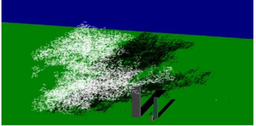
Figure 35: Cumulus cloud formation caused by vertical air movement. Spheres at bottom are designated heat sources.

5.3.2 STRATUS TYPE CLOUDS

Stratus clouds are formed slightly differently than cumulus clouds. Stratus clouds usually form over cold ocean water, with little or no vertical air movement. Contrary to the cumulus cloud set-up, for stratus clouds we do not define any additional heat source for our environment and our source of humidity is outside our simulation region, carried in on a high-velocity cross-wind. The user can define the direction and altitude of the crosswind and also the amount of humidity carried in by the wind. This gives us humidity generally traveling horizontally instead of vertically. When any of the water vapor condenses, the latent heat released causes some buoyancy and therefore we sometimes see wispy streaks of cloud, interspersed horizontally around the dew point. Figure 36 is an example of stratus cloud formation.

The above images were rendered interactively on a grid size of 15x50x15 at an approximate frame rate of 1 frame/sec. Frame rate can be increased to 7-10 frames/sec with a grid size of 15x15x15. We have used a Pentium III 800MHz processor with 256Mb RAM and a Geforce 2 graphics accelerator.

6 RESULTS AND PROBLEMS ENCOUNTERED

In this section we discuss the results of our study as well as present some of the problems that were encountered during the course of this research and their proposed solutions.

Many of the problems encountered are related to our application of the Navier-Stokes fluid model to the problem of atmospheric simulation. As we have previously

mentioned, we have assumed that density, and therefore pressure, are constant in our system in order to make the Navier-Stokes solution less expensive to compute. However, we have used empirical data to specify the pressure in our system, which is exponentially proportional to altitude, as shown in Figure 45 in Appendix A. Because our system is not solving for the variance in pressure over the space dimension, we must introduce additional steps to our simulation to account for the physical effects of this on the fluid flow in the atmosphere.

First, we realized that our system failed to account for expansion of the air during ascension. Because air experiences a decrease in density and thus pressure as we go up, the air expands to occupy a larger volume, and thus anything in the air such as water vapor or condensed particles will experience this expansive force. We have accounted for this in our system at a low-level by adding a step to our simulation pipeline. During this step, we analyze the entire velocity grid, and for every voxel with a positive vertical

velocity we add a proportional horizontal force22 in every surrounding direction. This concept is shown in two dimensions below in Figure 37. The net effect will be an expansive force added along the perimeter of any cells of vertical motion. Because we are tracing backwards when advecting our system, this expansive force on the perimeter of the cell will actually ‘pull-out’ density from this area, which gives the same effect as an internal expansive force ‘pushing out.’

Figure 37: Proposed expansion algorithm in two dimensions.

Furthermore, we found that our model also failed to properly conserve momentum in a system with density variance in the space dimension. As an air parcel rises, it collides with other air parcels above it. These higher air parcels have a lower density, thus the transfer of momentum between the two parcels results in an increase in upward velocity. We have also accounted for this at a low-level by adding a simulation step. At every time-step we analyze the velocity and we increase all positive vertical motion and decrease all negative vertical motion. This is shown visually in two dimensions in

22 _{The scale of this force should be experimentally determined. However we have not yet implemented}

Figure 38. We account for this because although there may be no local variation in density in our simulated atmosphere, we are solving for our fluid motion on a coarse grid and therefore there may be considerable variation in density from one voxel to another voxel at a higher/lower altitude. To ensure that momentum is conserved properly, we can recompute the Navier-Stokes solution at each voxel (using our altitude dependant pressure term) to ensure that error is within tolerance.

7

IMPLEMENTATION DETAILS

In this section we will discuss details of the implementation developed. All code discussed has been developed using OpenGL, GLUI, and C++ and has been written and tested on an 800MHz PentiumIII with 256Mb RAM and a Geforce2 graphics

accelerator. A version of this implementation is also available for UNIX.

7.1 DATA STRUCTURE

The fields we have in this simulation are humidity, heat, and condensation. In order to keep track of the different fields (e.g. humidity, condensation) that are being advected within our simulation, we have developed a data structure which contains the relevant information for each field. This data element is called a `Field' and contains a pointer to the three-dimensional grid structure that contains the mass distribution for the current field, as well as a pointer to the velocity field being used. Also contained within the Field structure are several constants used in the simulation such as diffusion rate, a resistance factor used to scale the motion of the vector field, and a gravity term for the field.

7.2 VISUALIZATION

Our simulation uses OpenGL to visualize our data. We display one field of data (either humidity, heat, or condensation) at each step in the simulation. The data is displayed using semi-transparent smooth-blended quadrilateral strips oriented from back to front with respect to the current view. Other visualization packages could also be used, however we have chosen OpenGL because of its portability.

7.3 SIMULATION

At each step in the simulation, we perform three basic operations — we advect the mass within the system using the current velocity field, we diffuse each field according to the diffusion rate defined for each field as well as the velocity field. We then execute a projection step which ensures that our system is divergence free with respect to pressure. The simulation steps are shown visually in Figure 39.

Figure 39: Simulation pipeline.

7.4 CONSTRAINTS

Most of the computational expenses in our method were a result of the cost of the fluid solver. The graphics processor we used, a Nvidia Geforce2 with 32Mb video memory, was adequate for this application. No bottlenecks were experienced when the system was rendering, only when executing the fluid solver. In our implementation we were unable to allocate a grid size larger than 25x25x50. However, with increased CPU speed and memory, which are both becoming increasingly more common on standard desktop PC’s, we would be able to increase both grid size and performance. We would like to test our application on a more powerful machine, such as a 2GHz PC with 1+Gb RAM. We would like to be able to run the simulation on a grid size of approximately 50x50x100 with interactive frame rates.

8 FUTURE WORK

In this section we discuss several directions for further research.

• More cloud types

There are many more types of cloud formations than just the two we have addressed in our current simulation. These include cirrus, cirrocumulus, cirrostratus, altocumulus, altostratus, nimbostratus, stratocumulus, and finally cumulonimbus [Wallen 1992]. As the names suggest, many of these cloud types are variations of the three main cloud formations: stratus, cumulus, and cirrus. Although we have not yet explored creation of these other types, we believe our model should easily adapt to handle them. With additional research we would like to add environmental presets for each cloud type to aid the user in creating these different base types.

• Complete growth cycle including precipitation and dissipation

We also hope to add to the current growth cycle of our clouds. Once enough water vapor has condensed into cloud form, gravity starts to pull down on some of the larger condensed particles. As the large droplets fall through the cloud colliding with other condensed particles, the process of precipitation begins [Wallen 1992]. We would like to experiment with modeling the precipitation stage of the cloud life cycle in our model. This model could be implemented simply by overlaying a

simple particle system on top of our volumetric cloud data. Because the

continuous collision model provides a statistical distribution of particle size in the cloud, we would not have to perform the more expensive collision detection algorithms in order to reproduce the process. However, some research may be required in order to develop an accurate algorithm for computing collision

probability under varying environmental conditions. This would not only include rain but also other forms of precipitation including snow and frozen rain.

• More research into atmospheric model

By improving our model of the atmosphere, we will be able to better mimic the complex processes that contribute to the formation of other cloud types and storm systems. We would like to improve our model to the point that we are able to successfully incorporate all three stages of the thunderstorm lifecycle described by Byers and Braham [1949]: the cumulus stage, the mature stage, and the downdraft stage.

• Gesture interface for artistic creation of environment

We would like to conduct some user experiments with a three-dimensional augmented reality interface in which the user is able to interact with the

environment by means of a gesture-based interface. Using such an interface the user would be able to more accurately shape the volumetric structure of the cloud during the course of the simulation.

• Modeling of nebulous clouds in deep space

We have also considered in the future applying this model to the formation and evolution of nebulous gas clouds in deep space. Our model would require

modifications to match the different environment and properties of gas flow in the zero-gravity vacuum of deep space.

• Application to high-level atmospheric simulation

We believe that this model could be applied to a high-level atmospheric simulator that could be used to visually simulate a section of the atmosphere equivalent to a 360° view from a point on Earth. The high-level simulator could use atmospheric data to determine where clouds might form and what type of clouds would form there. The low-level simulator (presented in this paper) could then be used to generate a local cloud of the correct type.

9 CONCLUSIONS

We have developed an efficient physically-based simulation of cloud formation which can be run interactively on a standard desktop PC with an average video

accelerator. This model provides a basis for modeling clouds in 3D using a computational fluid solver. We believe that the proposed model is a significant improvement over previous models of cloud formation in the field of Computer Graphics because of our use of an efficient three dimensional fluid solver and our detailed analysis of the physical process of atmospheric cloud formation. We hope to improve this model in the future by proceeding in the directions set out in section 8.

REFERENCES

Blinn, J. 1982. Light Reflection Functions for Simulation of Clouds and Dusty Surfaces. Proc. of SIGGRAPH '82, pp.21–29.

Braham Jr., R.R. 1996. The Thunderstorm Project. Bulletin of the American Meteorological Society, 77,8.

Brower Jr., W. B. 1999. A Primer in Fluid Mechanics: Dynamics of Flows in One Space Dimension. CRC Press, Boca-Raton, FL.

Byers, H. R. and Braham Jr., R.R. 1949. The Thunderstorm. U.S. Department of Commerce, Washington D.C. 287pp.

Dobashi, Y., Kaneda, K., Yamashita, H., Okita, T., and Nishita, T. 2000. A Simple, Efficient Method for Realistic Animation of Clouds. Proc. of SIGGRAPH 00, pp.19–28.

Ebert, D.S. 1997. Volumetric Modeling with Implicit Functions: A Cloud is Born. Visual Proc. of SIGGRAPH '97, pp. 147.

Fedkiw, R., Stam, J., and Wann Jensen, H. 2001. Visual Simulation of Smoke. Proc. of SIGGRAPH 01, pp. 15–22.

Foster, N. and Fedkiw, R. 2001. Practical Animation of Liquids. Proc. of SIGGRAPH '01, pp. 23–30.

Foster, N. and Metaxas, D. 1997. Modeling the Motion of a Hot, Turbulent Gas. Computer Graphics. 31,181–188.

Gardner, G. 1985. Visual Simulation of Clouds. Proc. of SIGGRAPH '85, pp. 297–303. Harris, M. J. and Lastra, A. 2001. Real-Time Cloud Rendering. Computer Graphics

Forum (Eurographics '01 Proc.), 20,3.

Kajiya, J. and Von Herzen, B. 1984. Ray Tracing Volume Densities. Proc. of SIGGRAPH '84, pp. 165–174.

Kaneko, K. 1990. Simulating Physics with Coupled Map Lattices---Pattern Dynamics, Information Flow, and Thermodynamics of Spatiotemporal Chaos. World Scientific, 1. Singapore.

Levoy, M. 1990. Efficient Ray Tracing of Volume Data. ACM Transactions on Graphics, 9,3,245–261.

Lewis, J. 1989. Algorithms for Solid Noise Synthesis. Proc. of SIGGRAPH '89, pp. 263–270.

Lide, D. R. 1992. CRC Handbook of Chemistry and Physics. CRC Press, Boca-Raton, FL. 72nd Ed.

Max, N. 1986. Atmospheric Illumination and Shadows. Proc. of SIGGRAPH ’86, pp. 117–124.

Miyazaki, R., Yoshida, S., Dobashi, Y., and Nishita, T. 2001. A Method for Modeling Clouds based on Atmospheric Fluid Dynamics. Proc. of Pacific Graphics ‘01, pp. 363–372.

Nagel, K. and Raschke, E. 1992. Self-organizing Criticality in Cloud Formation? Physica A, (182):519–531.

Neyret, F. 1997. Qualitative Simulation of Convective Clouds Formation and Evolution. Computer Animation and Simulation '97. pp. 113–124.

Perlin, K. 1989. Hypertexture. Proc. of SIGGRAPH '89, pp. 253–261.

Reeves, W. T. 1983. Particle Systems—A Technique for Modeling a Class of Fuzzy Objects. ACM Transactions on Graphics, 2,2,91–108.

Stam, J. and Fiume, E. 1995. Depiction of Fire and Other Gaseous Phenomena Using Diffusion Processes. Proc. of SIGGRAPH '95, pp. 129–136.

Stam, J. 1999. Stable Fluids. Proc. of SIGGRAPH 99, pp. 121–128.

Steinhoff, J. and Underhill, D. 1994. Modification of the Euler Equations for "Vorticity Confinement": Application to the Computation of Interacting Vortex Rings.

Physics of Fluids, 6,8,2738–2744.

Wallace, J. and Hobbs, P. 1977. Atmospheric Science: An Introductory Survey. Academic Press, New York, NY.

Wallen, R. N. 1992. Introduction to Physical Geography. Wm. C. Brown Publishers, Dubuque, IA.

SUPPLEMENTAL SOURCES CONSULTED

Foley, J., van Dam, A., Feiner, S., Hughes, J., and Phillips, R. 1993. Introduction to Computer Graphics. Addison-Wesley, Reading, MA.

Woo, M., Neider, J., Davis, T., and Shreiner, D. 1999. OpenGL Programming Guide, Third Edition. Addison-Wesley, Reading, MA.

APPENDIX A — ADDITIONAL IMAGES

Figure 40: Clouds generated and rendered using Dobashi method. Taken from early prototype model.

APPENDIX B — SEQUENTIAL IMAGES

Figure 42: Humidity field being advected by buoyancy.

Figure 43: Heat field. Notice added heat where condensation occurs.

APPENDIX C — PSEUDOCODE

The basic steps of our simulation:

• Initialize grid space. Initialize each voxel's:

o Velocity

o Humidity

o Heat

o Condensation

• Simulation Loop:

o Source Step. Add external velocity forces based on:

ƒ Wind

ƒ Vorticity Confinement

ƒ Buoyancy

o Simulation Step. Handles motion of fluid based on Stam's

model [Stam 1999]

ƒ Transport Step -- Handle Periodic Boundaries

ƒ Diffusion/Dissipation Step

ƒ Momentum Conservation Step

ƒ Expansion Step

ƒ Projection Step

o Compute relative humidity

o Condense water

ƒ Compute condensation

ƒ Reduce humidity

APPENDIX D — ATMOSPHERIC TABLES

Figure 45: Chart of pressure vs. altitude in troposphere

APPENDIX E — USEFUL TERMS

Buoyancy — An upward force caused by differences in temperature and density of air. Dew Point — The temperature at which a rising air parcel reaches saturation and

condensation begins.

Hygroscopic Nuclei — Tiny particles in the air upon which water can condense to form clouds.

Kinematic viscosity —The fluidic viscosity of the material over the density [White 1991].

Relative Humidity — The ratio of water vapor currently held by a constant volume of air to the total amount of water vapor that volume could hold at maximum.

Tropopause — The upper boundary of the tropopause.

Troposphere — The lower 12 km of the atmosphere. Also known as the zone of weather.