ISTANBUL TECHNICAL UNIVERSITYFINSTITUTE OF SCIENCE AND TECHNOLOGY
WAVE POWER POTENTIAL ASSESSMENT OF AEGEAN SEA
M.Sc. THESIS Navid JADIDOLESLAM
Department of Civil Engineering
Hydraulic and Water Resources Engineering Programme
ISTANBUL TECHNICAL UNIVERSITYFINSTITUTE OF SCIENCE AND TECHNOLOGY
WAVE POWER POTENTIAL ASSESSMENT OF AEGEAN SEA
M.Sc. THESIS Navid JADIDOLESLAM
(501121517)
Department of Civil Engineering
Hydraulic and Water Resources Engineering Programme
Thesis Advisor: Assoc. Prof. Mehmet ÖZGER
˙ISTANBUL TEKN˙IK ÜN˙IVERS˙ITES˙IFFEN B˙IL˙IMLER˙I ENST˙ITÜSÜ
EGE DEN˙IZ˙IN˙IN DALGA GÜCÜ POTANS˙IYEL˙IN˙IN BEL˙IRLENMES˙I
YÜKSEK L˙ISANS TEZ˙I Navid JADIDOLESLAM
(501121517)
˙In¸saat Mühendisli˘gi Anabilim Dalı Hidrolik ve Su Kaynakları Programı
Tez Danı¸smanı: Assoc. Prof. Mehmet ÖZGER
Navid JADIDOLESLAM, a M.Sc. student of ITU Institute of Science and Technol-ogy 501121517 successfully defended the thesis entitled“WAVE POWER POTEN-TIAL ASSESSMENT OF AEGEAN SEA”, which he prepared after fulfilling the requirements specified in the associated legislations, before the jury whose signatures are below.
Thesis Advisor : Assoc. Prof. Mehmet ÖZGER ... Istanbul Technical University
Jury Members : Asst. Prof Ali UYUMAZ ... Istanbul Technical University
Asst. Prof Ali Osman PEKTA ¸S ... Bahçe¸sehir University
Date of Submission : 3 May 2014 Date of Defense : 29 May 2014
FOREWORD
This thesis is supported by TÜB˙ITAK and prepared in Hydraulic and Water Resources Engineering Laboratory of Istanbul Technical University. Great effort has been spent on modeling with MIKE 21 SW software and specially for data analysis. The thesis is written by using LaTeX word processing program.
Most of all, I wish to thank my supervisor, Assoc. Prof. Mehmet ÖZGER, for giving me the chance to perform this work and to have guided and helped me through the whole MSc. process. His supervision and advises have made it a great and positive experience. I owe my thanks to Prof. Dr. Necati A ˘GIRAL˙IO ˘GLU for his precious helps and guidance.
Furthermore, I would like to express my gratitude to all the other colleagues at the Hydraulic and Water Resources Engineering Laboratory that have helped me and made this study such a pleasant journey.
Finally, I would like to give my special thanks to my parents and my friends. Their motivation and continuous support have made this happen and more than enjoyable. I am very grateful for everything you have done for me.
TABLE OF CONTENTS Page FOREWORD... ix TABLE OF CONTENTS... xi ABBREVIATIONS ... xiii LIST OF TABLES ... xv
LIST OF FIGURES ...xvii
SUMMARY ... xxi ÖZET ...xxiii 1. INTRODUCTION ... 1 1.1 Purpose of Thesis ... 3 1.2 Literature Review ... 4 2. DATA... 11 2.1 Geometry of Domain ... 11 2.2 Boundary Conditions... 13 2.3 Mesh Generation ... 14 2.4 Bathymetry Data... 16 2.5 ECMWF Data ... 16
2.5.1 ERA-Interim wind data ... 19
2.5.2 Preparation of wind data... 19
2.6 Measured Data... 21
2.6.1 Buoy data of NATO-TU waves project ... 23
2.6.2 POSEIDON wave buoys data ... 23
3. MODEL VALIDATION ... 27 3.1 MIKE 21 SW ... 27 3.1.1 MIKE 21 SW features ... 28 3.2 Definitions ... 28 3.3 Model Parameters ... 32 3.3.1 Source functions ... 32 3.3.2 Basic equations ... 32
3.3.3 Wave action conservation equations... 34
3.3.4 Spectral discretizaion... 35
3.3.4.1 Frequency discretization ... 35
3.3.4.2 Directional discretization... 35
3.3.4.3 Separation of wind-sea and swell ... 35
3.3.5.1 Algorithms for discretization in geographical and spectral domain ... 36 3.3.5.2 Propagation step... 37 3.3.6 Wind forcing... 38 3.3.7 Energy transfer ... 38 3.3.8 Wave breaking ... 39 3.3.9 Bottom friction ... 39 3.3.10 White-capping ... 39
3.3.11 Parameters used in model ... 42
3.4 Model Output Formats ... 42
3.5 Calibration Results ... 42
4. RESULTS AND DISCUSSIONS ... 55
4.1 Temporal Analyses ... 55
4.1.1 Monthly analysis ... 57
4.1.2 Seasonal analysis ... 83
4.1.3 Yearly analysis... 86
4.2 Spatial Analyses ... 86
4.2.1 Overall area-based analysis ... 86
4.2.1.1 Seasonal area-based analysis ... 88
4.2.2 Nearshore analysis... 90
4.2.3 Point series analysis... 92
4.2.3.1 Frequency analysis... 92
4.2.3.2 Monthly mean time series... 94
4.2.3.3 Wave rose analysis ... 96
5. CONCLUSION ... 99 REFERENCES... 103 APPENDICES ... 107 APPENDIX A ... 109 APPENDIX B... 117 CURRICULUM VITAE ... 123
ABBREVIATIONS
ANFIS :Adaptive-Network-Based Fuzzy Inference System BCM :Billion Cubic Meters
DDP :Directional Decoupled Parametric DHI :Danish Hydraulic Institute
ECMWF :European Center for Medium-Range Weather Forecasts GEODAS :GEOphysical DAta System
GFS :Global Forecast System
GSHHS :Global Self-consistent, Hierarchical, High-resolution Shoreline HCMR :Hellenic Center for Marine Research
IPCC :Intergovernmental Panel on Climate Change NCEP :National Center for Environmental Prediction NDBC :National Data Buoy Center
NGDC :National Geophysical Data Center
NOAA :National Oceanic and Atmospheric Administration REMO :Regional Atmosphere Model
SWAN :Simulating Waves Near-shore TPE :Tonne Petroleum Equivalent
TÜB˙ITAK :The Scientific And Technological Research Council of Turkey WAMC4 :WAve Model Cycle 4
WEC :World Energy Council WRI :World Resource Institute
LIST OF TABLES
Page
Table 1.1 : Turkey’s energy supply in 2009, 2010 and 2011. ... 2
Table 2.1 : List of coastline data resources. ... 11
Table 2.2 : A sample boundary conditions definition file content. ... 12
Table 2.3 : Format for MIKE DFS2 files. ... 22
Table 2.4 : Specifications of wave buoys used in calibration. ... 25
Table 3.1 : Model parameters specified after calibration... 41
Table 3.2 : Statistical Evaluations on Significant Wave Height... 54
Table 3.3 : Statistical evaluations on Mean Wave Period. ... 54
Table 4.1 : Time steps and duration of every month for normal year. ... 74
Table 4.2 : Time steps starts and end and duration of each month for a leap year. 74 Table 4.3 : Fifteen-year mean significant wave height and mean wave power area percentages in domain... 88
Table 4.4 : Significant wave height and wave power percentages based on 15 years spring season simulation data... 89
Table 4.5 : Significant wave height and wave power percentages based on 15 years summer simulation data... 89
Table 4.6 : Significant wave height and wave power percentages based on fall season simulation. ... 90
Table 4.7 : Significant wave height and wave power percentages based winter season simulation. ... 91
Table 4.8 : Mean significant wave height and mean wave power on the parallel shape of the east coast of Aegean Sea. ... 91
Table 4.9 : Coordinates of the selected points for in-depth investigations. ... 92
Table 4.10 : Fifteen-year mean wave height and wave period values for selected points... 95
LIST OF FIGURES
Page Figure 2.1 :Geometry of the Aegean Sea and nodes and vertices used in mesh
generation process... 13
Figure 2.2 :Boundary conditions of the domain. ... 14
Figure 2.3 :General view of unstructured mesh used for the Aegean Sea. ... 15
Figure 2.4 :Detailed view of the bathymetry in eastern coasts of Aegean Sea... 17
Figure 2.5 :Bathymetry map of the domain. ... 18
Figure 2.6 :Sort of wind speed matrices in 2 directions. ... 20
Figure 2.7 :Visual basic code for cell selection in excel and data organization. ... 21
Figure 2.8 :Visual basic code for building z in excel and data organization. ... 22
Figure 2.9 :DFS2 wind data view in MIKE Zero data viewer. ... 22
Figure 2.10 :Sample image of measured data plotted in GIF file format by NATO-TU Waves. ... 24
Figure 2.11 :General view of the digitization steps of the NATO-TU Waves plotted data with Get Data Graph Digitizer. ... 24
Figure 3.1 :Locations of the buoys in Aegean Sea used as measured data... 43
Figure 3.2 :Comparison of the simulated and measured significant wave height for Athos station... 44
Figure 3.3 :Comparison of the simulated and measured mean wave period for Athos station. ... 44
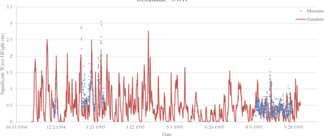
Figure 3.4 :Comparison of the simulated and measured significant wave height for Bozcaada station... 45
Figure 3.5 :Comparison of the simulated and measured mean wave period for Bozcaada station. ... 45
Figure 3.6 :Comparison of the simulated and measured significant wave height for Dalaman station... 46
Figure 3.7 :Comparison of the simulated and measured mean wave period for Dalaman station. ... 46
Figure 3.8 :Comparison of the simulated and measured significant wave height for E1M3A station. ... 47
Figure 3.9 :Comparison of the simulated and measured mean wave period for E1M3A station. ... 48
Figure 3.10 :Comparison of the simulated and measured significant wave height for Lesvos station. ... 48
Figure 3.11 :Comparison of the simulated and measured mean wave period for Lesvos station... 49
Figure 3.12 :Comparison of the simulated and measured significant wave height for Mykonos station. ... 49
Figure 3.13 :Comparison of the simulated and measured mean wave period for
Mykonos station... 50
Figure 3.14 :Comparison of the simulated and measured significant wave height for Santorini station... 50
Figure 3.15 :Comparison of the simulated and measured mean wave period for Santorini station. ... 51
Figure 3.16 :Comparison of the simulated and measured significant wave height for Saronikos station. ... 51
Figure 3.17 :Comparison of the simulated and measured mean wave period for Saronikos station. ... 52
Figure 3.18 :Comparison of the simulated and measured significant wave height for Skyros station. ... 52
Figure 3.19 :Comparison of the simulated and measured mean wave period for Skyros station... 53
Figure 4.1 :Fifteen-year mean significant wave height for Aegean Sea. ... 56
Figure 4.3 :Fifteen-year mean significant wave height for January. ... 58
Figure 4.4 :Fifteen-year mean wave power for January... 59
Figure 4.5 :Fifteen-year mean significant wave height for February. ... 60
Figure 4.6 :Fifteen-year mean wave power for February... 61
Figure 4.7 :Fifteen-year mean significant wave height for March... 62
Figure 4.8 :Fifteen-year mean wave power for March. ... 63
Figure 4.9 :Fifteen-year mean significant wave height for April... 64
Figure 4.10 :Fifteen-year mean wave power for April. ... 65
Figure 4.11 :Fifteen-year mean significant wave height for May. ... 66
Figure 4.12 :Fifteen-year mean wave power for May... 67
Figure 4.13 :Fifteen-year mean significant wave height for June... 68
Figure 4.14 :Fifteen-year mean wave power for June... 69
Figure 4.15 :Fifteen-year mean significant wave height for July... 70
Figure 4.16 :Fifteen-year mean wave power for July. ... 71
Figure 4.17 :Fifteen-year mean significant wave height for August... 72
Figure 4.18 :Fifteen-year mean wave power for August. ... 73
Figure 4.2 :Fifteen-year mean wave power for Aegean Sea. ... 75
Figure 4.19 :Fifteen-year mean significant wave height for September. ... 76
Figure 4.20 :Fifteen-year mean wave power for September. ... 77
Figure 4.21 :Fifteen-year mean significant wave height for October. ... 78
Figure 4.22 :Fifteen-year mean wave power for October. ... 79
Figure 4.23 :Fifteen-year mean significant wave height for November... 80
Figure 4.24 :Fifteen-year mean wave power for November. ... 81
Figure 4.25 :Fifteen-year mean significant wave height for December. ... 82
Figure 4.26 :Fifteen-year mean wave power for December... 83
Figure 4.27 :Mean significant wave height for Spring... 85
Figure 4.28 :Mean significant wave height for Summer. ... 85
Figure 4.31 :Mean wave power for Spring. ... 87
Figure 4.32 :Mean wave power for Summer... 87
Figure 4.33 :Mean wave power for Fall... 87
Figure 4.34 :Mean wave power for Winter. ... 87
Figure 4.35 :Selected points in Aegean Sea... 93
Figure 4.36 :Monthly mean significant wave heights for selected points... 94
Figure 4.37 :Monthly mean wave periods for selected points. ... 95
Figure 4.38 :Wave rose diagrams for selected points. ... 98
Figure A.1 :Mean SWH - 1999... 110
Figure A.2 :Mean SWH - 2000... 110
Figure A.3 :Mean SWH - 2001... 110
Figure A.4 :Mean SWH - 2002... 110
Figure A.5 :Mean SWH - 2003... 110
Figure A.6 :Mean SWH - 2004... 110
Figure A.7 :Mean SWH - 2005... 111
Figure A.8 :Mean SWH - 2006... 111
Figure A.9 :Mean SWH - 2007... 111
Figure A.10:Mean SWH - 2008... 111
Figure A.11:Mean SWH - 2009... 111
Figure A.12:Mean SWH - 2010... 111
Figure A.13:Mean SWH - 2011... 112
Figure A.14:Mean SWH - 2012... 112
Figure A.15:Mean SWH - 2013... 112
Figure A.16:Mean wave power - 1999. ... 113
Figure A.17:Mean wave power - 2000. ... 113
Figure A.18:Mean wave power - 2001. ... 113
Figure A.19:Mean wave power - 2002. ... 113
Figure A.20:Mean wave power - 2003. ... 113
Figure A.21:Mean wave power - 2004. ... 113
Figure A.22:Mean wave power - 2005. ... 114
Figure A.23:Mean wave power - 2006. ... 114
Figure A.24:Mean wave power - 2007. ... 114
Figure A.25:Mean wave power - 2008. ... 114
Figure A.26:Mean wave power - 2009. ... 114
Figure A.27:Mean wave power - 2010. ... 114
Figure A.28:Mean wave power - 2011. ... 115
Figure A.29:Mean wave power - 2012. ... 115
Figure A.30:Mean wave power - 2013. ... 115
Figure B.1 :Significant wave height and mean wave period frequency diagram for point 1... 117
Figure B.2 :Significant wave height and mean wave period frequency diagram for point 2... 117
Figure B.3 :Significant wave height and mean wave period frequency diagram for point 3... 118
Figure B.4 :Significant wave height and mean wave period frequency diagram for point 4... 118 Figure B.5 :Significant wave height and mean wave period frequency diagram
for point 5... 119 Figure B.6 :Significant wave height and mean wave period frequency diagram
for point 6... 119 Figure B.7 :Significant wave height and mean wave period frequency diagram
for point 7... 119 Figure B.8 :Significant wave height and mean wave period frequency diagram
for point 8... 120 Figure B.9 :Significant wave height and mean wave period frequency diagram
for point 9... 120 Figure B.10:Significant wave height and mean wave period frequency diagram
WAVE POWER POTENTIAL ASSESSMENT OF AEGEAN SEA
SUMMARY
In this study the wave power in Aegean Sea was simulated over the period from 1999 to 2013 using a third-generation spectral wave model MIKE 21 SW.
The model is built in MIKE Zero mesh generator and the mesh consists of 5927 nodes and 10081 elements. Bathymetry data obtained from NOAA and Significant Wave Height and Mean Wave Period of the 5 stations: Dalaman, Bozcaada obtained from NATO-TU WAVES and Athos, E1M3A and Saronikos originally taken from HCMR database.
Wind data with 0.125◦×0.125◦ resolution for every 6h interval was obtained from ECMWF (Era-Interim) database. The wave model calibrated by 5 buoy stations measurements and the generated wave characteristics such as significant wave height and mean wave period gave a high accuracy of the model.
Wave power atlas was generated based on an averaged 15 years wave data obtained from model. Near Turkish coast, mean wave power found 2 kW/m depending on the way of the waves, waves traveling after islands have less power in Turkish coasts. Wave power in the middle Aegean have higher wave power potentials compared to coastal regions where the calculated mean wave power in this area is more than 4 kW/m. Maximum mean wave power observed from simulations are located in 2 locations between Ikaria and Mykonos islands and between Kasos and Crete islands reaching 5.2 kW/m.
Results of the seasonal analysis in this study demonstrate that the maximum wave power values in winter occurs in northern part of the Aegean Sea with more than 8 kW/m. Maximum mean wave power occurrence location from winter to spring changes from north to middle southern part of the study region, between Crete and Kasos islands.
The western and middle part of study area found to have least and most wave power potential respectively.
For the Turkish coast it was seen that the shading effect had decreased the wave energy for this regions. Though there were some locations which had a higher wave power potential compared with other parts of east coast of Aegean Sea.
In a glance to the 15-year mean significant wave height map it was seen that high wave potential is available in Northern part of Aegean Sea specially in Bozcaada, Gökçeada and Baba Burnu. In this part mean wave power is between 1.0 - 2.8 kW/m.
For middle-Aegean Sea, Karaburun and Çesme have a 2.0 kW/m of wave power potential.
EGE DEN˙IZ˙IN˙IN DALGA GÜCÜ POTANS˙IYEL˙IN˙IN BEL˙IRLENMES˙I
ÖZET
Türkiye enerji kullanımında %74 oranında dı¸sa ba˘gımlıdır. Bu oranın 2020 yılına kadar % 80 civarında olaca˘gı enerji ile ilgilenen yöneticiler ve otoriteler tarafından tahmin edilmektedir.
Enerji tüketiminde dı¸sa ba˘gımlılı˘gın, Türkiye’nin jeopolitik konumu dikkate alındı˘gında her an yaptırım aracı veyahut ambargo malzemesi olarak kullanılabilme olasılı˘gı yüksektir.
Büyük hidroelektrik santraller çevre acısından temiz olmasına kar¸sın, canlı hayat alanlarını kısıtlamakta ve bazen eko sistem üzerinde zararlı etkiler ortaya koyabilmektedir. Türkiye, eldeki verilere göre her yıl enerji tüketiminde artı¸sla kar¸sıla¸sıyor ve bu rakamlar gittikçe artıyor.
Dalga enerjisinin temiz ve güç kayna˘gının yenilenebilir olması dünya üzerinde ilgiyi bu yöne do˘gru ta¸sımaktadır. Özellikle, Amerika, Kanada, ˙Ingiltere, Kuzey Avrupa Ülkeleri, ˙Ispanya ve Portekiz çok ciddi yatırımlar ve te¸svikler vererek dalga enerjisinden faydalanma hususunda önemli ara¸stırmalar yapmaktadırlar. Örne˘gin, ¸su an ˙Ispanya’nın Bask bölgesinde bulunan Mutriku yerle¸sim yerinde dalga enerjisi dönü¸süm santrali ile enerji ihtiyacı bütünüyle kar¸sılamaktadır.
Hükümetler arası ˙Iklim De˘gi¸sikli˘gi Panelinin verilerine göre küresel enerji ihtiyacının % 30’nun deniz dalgalarının hareket enerjisinden kar¸sılanması mümkündür.
Dünya da önde giden ülkelerden geriye kalmamak için enerji üretiminde yeni yöntemler kullanmak ve uygulamak gerekir ki bu kapsamda bilimsel ara¸stırma her uygulamadan daha çok önem ta¸sır.
Birinci adımda Ege Denizi için çalı¸sma sınırları belirlenerek ve harita üzerinde sınır ¸sartları seçilmi¸stir. Kıyı çizgisi verileri de˘gi¸sik kaynaklardan bulabilmektedir. Bu kaynaklardan en hassas ve en çok kullanılanı seçilmi¸stir.
MIKE 21 SW’de kurulan benze¸stirmede kullanılan bir di˘ger veri ise rüzgâr verisidir. Ege Denizini kapsayan alan için 1999-2013 yılları arasında 6 saatlik zaman aralıklarına sahip rüzgâr hızları “x” ve “y” bile¸senleri olarak ECMWF’den elde edilmi¸stir.
A˘g üretimi projenin di˘ger adımlarından daha fazla önem ta¸sır. Düzenli ve uygun bir a˘g üretimi yapabilmek ileri adımlarda ya¸sanacak problemlerinde önüne geçecektir. A˘g üretiminin hem batimetre interpolasyonunda hem de hesaplamalarda etkisi büyük oldu˘gundan uygun bir a˘g yüksek ba¸sarılı bir modele sebep olacaktır.
Bu tez’de kullanılan batimetri verilerinin çözünürlükleri 0.004◦ (400 m)’dir. Veriler, XYZ dosya formatında A˘g üretici modülüne yüklenerek dikkatle incelenmi¸s ve düzenlenmi¸stir. Bu kapsamda kıyı çizgisinin arkasında kalan bazı noktalar elenmi¸stir.
MIKE 21 SW’de kurulan benze¸stirmede kullanılan bir di˘ger veri ise rüzgâr verisidir. Ege Denizini kapsayan alan için 1999-2013 yılları arasında 6 saatlik zaman aralıklarına sahip rüzgâr hızları “x” ve “y” bile¸senleri olarak ECMWF’den elde edilmi¸stir.
Elde edilen rüzgâr verisi 0.125 derece çözünürlükte olup, 6 saatlik zaman dilimlerini kapsamaktadır. Rüzgâr verileri mevcut olan en yüksek çözünürlükte olup ECMWF’in ERA-Interim yeniden analizleri ile üretilmi¸stir.
Bu çalı¸smada, 1999-2013 dönemi için üçüncü nesil olan spektral dalga modeli MIKE 21 SW’i kullanarak Ege Denizinin dalga gücü incelenmi¸stir. Bu modellemede ilgili bölgede mevcut çoklu yüzen istasyon verileri kullanılmı¸stır.
Bu istasyonlar Dalaman, Bozcaada, Athos, E1M3A, Lesvos, Mykonos, Santorini, Saronikos ve Skyros’dan ibaretler.
Dalaman ve Bozcaada istasyonlarının ölçülmü¸s verileri NATO-TU WAVES Projesin-den alınmı¸stır ve di˘ger istasyonlar yunanistanın tarafından yönetilen kurum HCMR tarafından temin edilmi¸stir.
Kalibrasyon için kullanılan 9 istasyon için bulunmu¸s olan istastistik de˘ger-lerndirmelerin neticesinde modelin güvenilebilirli˘gi denetilmi¸stir ve modelin yüksek dayanabilirli˘gi ortaya konulmu¸stur.
Bu çalı¸smada belirgin dalga yüksekli˘gi için modelin verdi˘gi de˘gerler ve ölçülmü¸s de˘gerlerin korelasyon katsayıları yüksek derecede cevaplar vermi¸stir.
Bu model MIKE Zero A˘g üretimine dayanmaktadır. Bu a˘gın 5927 dü˘gümü ve 10081 elemanı vardır. Batimetre verileri NOAA’dan sa˘glanmı¸stır. Her 6 saat ara’ile 0.125◦×0.125◦ çözünürlükle rüzgar verileri ECMWF (Era-Interim) veri tabanından sa˘glanmı¸stır.
Dalga modeli 9 yüzen istasyondaki ölçümlerle kalibre edilmi¸stir. Belirgin dalga yüksekli˘gi ve ortalama dalga periyodu gibi dalga karakteristikleri modelde yüksek bir hassaslıkla hesaplanmı¸stır.
Kalibrasyonun hedefi, model parametrelerinin de˘gerlerini optimize etmektir. Bu parametrelerin kar¸sıla¸stırması için kullanılacak olan istatiksel ölçü indeksleri a¸sa˘gıda verilmi¸stir. Bu ölçü kriterleri kullanılarak elde edilen de˘gerler simülasyon sonuçları ve ölçüm de˘gerleri arasında yüksek bir korelasyon vardır.
Bu çalı¸smada, dalga modeli olu¸sturulması için DHI MIKE yazılımının MIKE 21 SW modülü kullanılmı¸stır. MIKE 21 SW, rüzgâr dalgalarının kıyıdan uzak ve kıyı yakınlarındaki büyüme, azalma ve transformasyonunu hesaplayan Danimarka Hidrolik Enstitüsü (DHI) tarafından geli¸stirilmi¸s ve dünya genelinde güvenilerek uygulanan bir yazılımdır. MIKE 21 SW a¸sa˘gıdaki fiziksel hesaplamaları kapsamaktadır.
Model sonuçları 6 saatlik hassasiyette sonuçlar vermektedir. Dolayısıyla 1999 yılında ba¸slayan ve 2013 yılına kadar devam eden süreçte 6 saatlik zaman çözünürlü˘günde belirgin dalga yüksekli˘gi ve dalga periyodu dalga özellikleri model çıktısı olarak elde edilmi¸stir.
Bu ara¸stırmada benze¸stirmeler 1999-2013 yıllarını kapsayan 15 yıllık bir süre için yapılmı¸stır. Her bir yıl için kalibre edilmi¸s parametreler ile model ayrı ayrı çalı¸stırılmı¸stır.
Bir yıllık zaman dilimi için modelin 16GB ram ve 2.2GHz i¸slemci hızına sahip bilgisayarda çalı¸sma süresi 30 saat sürmü¸stür. Yapılan 15 yıllık benze¸sim için toplam hesaplama süresi yakla¸sık 30 günde bitmi¸stir.
Yıllık sürelerle yapılmı¸s oldu˘gundan her yıl için farklı ortalama belirgin dalga yükseklikleri ve ortalama dalga gücü elde edilmi¸stir. Aylık de˘gerlerin ayırılması için zaman adımları belirlenmi¸s ve her yılın 12 ayı için dalga özellikleri teker teker çıkartılmı¸stır.
Ortalama 15 yıllık verilere dayanarak modelden dalga gücü atlası üretilmi¸stir. Türkiye kıyılarına yakın, dalgaların geli¸s yoluna ba˘glı olarak ortalama dalga gücü 2 kW/m bulunmu¸stur. Türkiye’nin adalara bakan kıyılarında, adalardan sonra kıyıya yakla¸san dalgaların daha gücü vardır.
Ege Denizinin orta kısımlarında, kıyı bölgesine göre daha yüksek dalga gücü potansiyeli mevcuttur. Bu kısımdaki dalga gücü 4 kW/m’den daha büyüktür. Model çalı¸smalarında hesaplanan en büyük ortalama dalga gücü iki yerde ortaya çıkmı¸stır. Bunlardan bir tanesi ˙Ikara ve Mykonos adaları arasında, di˘geri ise Kasos ve Crete adaları arasında meydana gelmi¸stir. Bu iki noktada maksimum ortalama dalga gücü 5.2 kW/m’ye ula¸smı¸stır.
Zaman incelemeleri aylar ve mevsimler göz önüne alınarak yapılırken mekân incelemelerinde bu parametrelerin çalı¸sma alanı içinde nasıl de˘gi¸sti˘gine bakılmı¸stır. Belirgin dalga yüksekli˘gi ve dalga gücü zaman ve mekânla de˘gi¸sim göstermektedir. Bu de˘gi¸simler çok belirgin olarak kar¸sımıza çıkmaktadır.
Dolayısıyla pratikte yapılacak bir çalı¸smada zaman ve mekân de˘gi¸sim da˘gılımına bakılması önem arz etmektedir. Kı¸s aylarında hem dalga yüksekli˘gi hem de dalga gücü di˘ger aylara göre çok yüksek de˘gerler vermektedir. En az güç potansiyeli ise yaz aylarında görülmü¸stür.
Belirgin dalga yüksekli˘gi ve dalga gücünün 15 yıllık aylık ortalamalarına bakıldı˘gında en yüksek de˘gerlerin ¸Subat ayında çıktı˘gı belirlenmi¸stir. ¸Subat ayında yer yer 9 kW/m kadar çıkan bir dalga gücü potansiyeli görülebilmektedir. Buna kar¸sın en dü¸sük de˘gerlerin ise Temmuz ve A˘gustos aylarında görüldü˘gü tespit edilmi¸stir.
Ege Denizinde bulunan adalar dalga olu¸sumunu engelledi˘gi için belirgin dalga yüksekli˘gi ve dalga gücü potansiyeli daha çok adaların bulunmadı˘gı bo¸s kısımlarda olu¸smaktadır.
Bu çalı¸smada mevsimlik analiz sonuçları 8 kW/m’den daha yüksek olarak Ege Denizinin kuzey kısmında, kı¸sın meydana geldi˘gini göstermi¸stir.
En büyük ortalama dalga gücü olu¸sma yeri, kı¸stan ilkbahara geçerken, çalı¸sma alanının kuzeyinden orta güney kısmına, yönü Crete ve Kasos adaları arasına kaymaktadır. Modelleme ile çalı¸sma alanının batısı ve ortasında sıra ile en dü¸sük ve en yüksek dalga gücü potansiyeli bulunmu¸stur.
1. INTRODUCTION
Water plays a crucial role in human life whereas 70 % of the Earth is covered with water that most of them are connected to each other forming oceans and seas. Waves are one of the most important elements of oceans and seas that carry mass and energy by them, sometimes traveling from a continent to another. Waves are different in magnitude depending on the source of their formation cause.
Natural resources are so important for every country’s economy. Best utilization of these resources can make a country nearly independent from outside of country. According to the WRI more than 80 % of the world countries have coastal line, while Turkey is surrounded by seas. This could be called as a chance for this country to get used from wave energy.
The green house gas effect of fossil fuels encouraged scientists and researchers to make a replacement for this kind of energy resources, so that green energy resources became more important than before in last century. Wave energy is one of the green energies available without the most of disadvantages of the fossil fuels had.
On the other hand behavior of waves in a basin is principal for future planning constructions in the region but measurement of the wave characteristics for a long period of time demand more budget to install measurement buoys in the interested area, so that simulation of the waves characteristics is like an economical answer to an expensive question.
There is a great wave energy potential throughout world which should be seen as a green energy resource that can be harvested in near future. Global wave power atlas [1]with a high accuracy of model which shows that world has a great wave energy in different districts and oceans which could be taken into account and used either by an individual national or multinational projects, so that more research and development is demanded for a higher precision of energy derivation from waves.
Table 1.1: Turkey’s energy supply in 2009, 2010 and 2011.
2009 (1000 TPE) 2010 (1000 TPE) 2011 (1000 TPE)
Coal 32,913 33,531 35,841 Natural Gas 32,775 34,907 36,909 Petroleum 30,565 29,221 30,499 Hydraulic 3,092 4,454 4,501 Wood 3,530 3,392 2,446 Geotherm etc. 1,250 1,391 14,63
Animal waste etc. 1,136 1,166 1,091
Geothermal 375 575 597
Solar 429 432 630
Wind 129 251 406
Biofuel 9 12 18
Total 106,138 109,266 114,480
Last century could be called as a population explosion in the world as the statistics show that world population has became 7 billion in 2011 from 2 billion in year 1927, this fact is similar in Turkey where it has reached 75 million from 13 million between 1927-2012 years. Population increase made Turkey to import 43 billion cubic meters of gas in year 2011, this statistic made Turkey 7th in the world top gas importers. More than 74% of the Turkey’s energy is imported , according to the energy executives and authority’s estimations this percentage would grow to reach 80% by year 2020. As it can be seen from Table 1.1 the statistical numbers of the Turkish Energy Ministry show that Turkey’s energy demand in 2011 was 114,480 Tones petroleum equivalent. Hydroelectric centrals can be a good green energy resource but they change the wildlife ecosystem and have other side effects. In the last decade there is a great enthusiasm for building wave energy converters and wave farms as a clean and renewable energy. Specially in United States, Canada, Britain, and northern European countries there are vast investments in this sector.
In 2005 the global electricity consumption was around 15 TW. With a total energy consumption of 131400 TWh/year According to the data of IPCC 30% of the global energy demand could be supplied by the energy of oceans and seas. According to the WEC, the global wave energy resource is estimated to be 1-10 TW.
characteristics’ distribution and magnitude throughout Aegean Sea while having detailed analysis on the obtained data from a 15 years period simulations done by a third generation spectral wave software which is produced by DHI. A deep study of the Aegean Sea can lead to a better decisions in later steps for investors in energy sector, so that this study’s aim was to make a complete reference of the Aegean Sea wave properties either in near shore and offshore locations.
1.1 Purpose of Thesis
The main purpose of the thesis which is funded by TÜB˙ITAK and it took 12 months of hard work, was to investigate the Aegean Sea’s 15-year mean wave power, locations of the maximum and minimum values, statistical analysis of the data obtained from simulations and comparing results of the model with the measured data and calibration of the model. This work is the result of deep study of the waves characteristics in this basin with detailed analysis and technical comments. Also the model constructed in this study could be used in future for other purposes like estimation of the waves in Aegean Sea for a short period of time by having an estimation of winds in this area.
• Main purpose
– Making a complete database of the wave’s characteristics for Aegean Sea – Spatial and temporal analysis for significant wave height and wave power – Deep study of the waves in Turkish coasts
• Literature review
– Making an abstract of the researches in regional aspect on wave power – Spectral wave modeling theoretical description
• Modeling
– Building a unstructured mesh for interested area – Application of MIKE 21 SW to Aegean Sea
• Calibration
– Digitization and organization of the measured data to be ready for calibration – Synchronization of the measured and simulated data
– Comparison of the observed data with the simulated data with statistical values
• Waves analysis
– Making 15-year, yearly, monthly and seasonal mean wave power atlases – Investigation of the wave power potential in east coasts of Aegean Sea – Wave rose and frequency analyses for important points in the study region. – Comparison of the waves in different distances from eastern coast of Aegean
Sea
1.2 Literature Review
By the rise of importance of wave energy and its beneficial aspects in world wide, every country has encouraged its researchers and scientists to invest their time on this subject. Therefore numerous researches have been conducted in recent years on wave power.
Hatada, Y. & Yamaguchi, M. (1998) applied 9 years ECMWF wind data with period from 1986 to 1994 to evaluate shallow water waves in Pacific coast of Japan. Wave estimation was done by a shallow water wave prediction model [2] which traces the change of directional spectrum along a refracted ray of each component focusing on a hindcast point is applied for long-year wave hindcasting in order to save computer processing time. In this study 6 buoy stations were used to verify model. Reasonable correlation coefficients were found by comparison of the measured and calculated data. Also in this study the result of simulation in the location of offshore station were more close to measured data in that point. On the other hand for waves higher than 2m a good agreement has reached between calculated and simulated wave heights [3].
model. The calibration of model resulted values 2, 0.8, 0.002 for white-capping, wave breaking, bottom friction parameters respectively. For extreme conditions analysis done by EVA software developed by DHI Water and Environment statistic distribution of the wind and wave data was most fitting to Truncated Gumble that gave less less standard deviation and smoother spatial pattern of extreme values. Some points adjacent to southern coast of Caspian sea were predicted by unrealistic values. These results were due to land interpolations were removed from results [4].
Jose & Stone (2006) investigated entire Gulf of Mexico’s wind generated wave and swell waves using MIKE 21 SW while the resolution of mesh used for coastal parts of this study is 2kma coarser grid of 30kmused for boundary. For Southern part of basin a bathymetric data with a 2.3kmresolution and for other parts 34.4kmresolution were used. Wind data was obtained from NCEP of NOAA. This is study is conducted with a period 36hrswhereas the comparisons between wave and wind data were done in both coastal and offshore parts of the domain. offshore station results demonstrated a close values to the measured however coastal station located in shallow water did not give a good calculated values for wind data measured, the effect of higher difference in wind data reflected in simulated wave values. The results of the study shows that during fair weather condition predicted wave parameters show a good correlation with measured data while this is not the same in the extreme weather conditions that estimated values are lower than measured. The diversity of the data could be related to the scale and accuracy of the input wind data [5].
Moeini & Etemad-Shahidi (2007) modeled Lake Erie’s wave characteristic located in North America. In this study simulations was done by MIKE 21 SW and SWAN then the comparisons and evaluations were taken part in this investigations. Wind data sets were obtained from National Data Buoy Center and 1 field data was obtained Marine Environmental Data Service which is hourly data sets. Comparisons between simulated data of SWAN model and results from Janssen wind input formulation [6] and cumulative steepness method were done and reached to good agreements. Results of the comparisons from SWAN and MIKE 21 SW demonstrate that SWAN model gives better results forHswhile MIKE 21 SW performs better in prediction ofTp. Also this study shows that using Komen’s formulation led to more accurate estimations of
Hswhile having less accurateTpresults from model. The cumulative steepness method for white-capping dissipation in SWAN model has a 2 times of Komen’s method [7] computational time so that it is not suggested to be used [8].
Kazeminezhad et al. (2007) evaluated neuro-fuzzy and numerical wave prediction models in Lake Ontario located in North America, where as used MIKE 21 spectral wave program and ANFIS for simulations. By application of the directional decoupled parametric formulation and fully spectral wave formulation which is based on the wave action conservation [9]. In DDP formulation, parameterization is made in the domain of frequency and first and zeroth moments of wave action is considered as dependent variable [10]. Domain consists of 1322 unstructured triangle elements and calibration took place with a 611 number of hourly wind and wave measurements. The buoy station is located in deep water, so that the only parameter calibrated is white-capping factor (c∗ds). The results show that MIKE 21 SW is performing more accurate in estimation of bothHs andTp[11] .
Cherneva et al. (2008) validated WAMC4 wave model for the Black Sea basin, wind data were obtained from regional atmosphere model(REMO) [12] [13] The spatial resolution for these simulations was chosen to be about 50×50kmand the simulated wind fields have been stored at every hour [14]. Validation is done with 4 different point measurements in the Black Sea and gratifying statistical results were obtained from model while showing that WAMC4 underestimates the significant wave height Hs in the case of rapid change of wind direction combined with low wind velocities. This model generally gave good agreements between output and measured data but model gives more accurate output as wind speed increases to a severe state [15] . Rusu (2009) calculated the wave power potential in Black Sea by both WAM and SWAN models for 1971 to 1994 by using wind data resolution of 0.25◦ and investigations done in Northern Black Sea. Analysis of the measured wave and wind data and comparison with model output values is taken part also in this study the wave characteristics were modeled by totally 4 different approach: 1. Komen’s parameterization [7], 2. Janssen’s model for atmospheric input [16] coupled with
atmospheric input [19] coupled with the saturation-based model of Alves and Banner for whitecapping [20]. Monthly mean wave direction for 8 directions and significant wave heightHs scatter table generated. The model is tested with 3 different stations, 2 buoy and 1 wave gauge. Reasonable correlation coefficients are derived from collations of methods; Alves and Banner’s method for white-capping gave the best results for significant wave heightsHsthrough all other models [21] .
G. Iglesias & R. Carballo (2009) modeled wave energy potential of the Death Coast in North Spain using WAM for offshore and SWAN for nearshore simulations. In this study 3 hourly hindcast wind from 1958 to 2001 is used. Wave data is computed by WAM cycle 4 forced with wind data of REMO for offshore locations and on the other hand coastal wave model is built on the SWAN model based on the wave action conservation [22]. The computational grid of this model is 0.150×0.150. The evaluation of the results were done by 16 SIMAR-44 site and 2 buoy measurements. It is concluded that mean wave power potential of the the study region is more than 40 kW/m, also it was found that significant wave heights are between 2 m and 5 m and wave periods of 11-14 s [23].
Arinaga & Cheung (2011) acquired global atlas of wave energy model by using WAVEWATCH 3 with 10 years (2000-2009) of NCEP’s Final Global Tropospheric Analysis (FNL) wind data which was obtained from Global Forecast System (GFS) [24]. This study has implemented WW3 with 1.25◦×1◦resolution of wind data and ice concentrations from National Ice Center. The separation of wind waves and swell is done in WW3. This study has validated it’s results with altimetry data of 6 different regions for a period of four and a half months from January 15 to May 24 2002, also 19 buoy measurement data is used to evaluate the model. Regression between altimetry data and model output has given a good correlation coefficient for significant wave height Hs and a RMSE of 0.36-0.48 m at 6 regions of the world. Mean wave period and peak wave period values simulated by the model do not have a agreeable closeness to measured values. Monthly median wave power of wind waves above 30◦N has a range 17-130 kW/m . The results also prove that the southern coasts of Australia and New Zealand are most appropriate for wave energy development, though
further investigation is needed wave energy infrastructures implementations for coastal regions [1] .
Liberti et al. (2013) studied wave energy resources in Mediterranean Sea with a more concentration on the west part of this sea. In this study which is conducted by 10 years (2001-2010) of wind data with a 0.125◦×0.125◦resolution obtained from ECMWF, more accurate model is built in contrast with the previous researches done for the region [25] [26] [27]. Simulations are done with 3rd-generation wave model WAM wave model cycle 4.5.3, domain’s discretization is done with a regular grid with 667×251 nodes in spherical coordinates. The domain consists of Mediterranean, Agean Seas while reaching to Italian coasts in the western part. Wind data resolution employed in this study is 0.25◦. The effects of currents and variations in sea surface elevation is neglected from calculations. The domain is considered as a closed basin. Wave characteristics are derived from model for every 3 hours and model values are calibrated with satellite and buoy measurements and statistical evaluations show a good results for calibrations. For further study of the wave behavior in the domain, 20 sites are selected in different parts of the domain for a deeper investigation. The most energetic parts of the Italian coastline is found to be in western coast of Sardinia and along the north-western and southern coast of Sicily [28].
Ayat (2013) created wave power atlas of Mediterranean and Aegean seas by using MIKE 21 SW, taking wind wave growth and nonlinear wave-wave interaction, dissipation due to white capping, bottom friction and depth-induced wave breaking refraction and shoaling. Triangular unstructured mesh is implemented in this study having 4098 nodes and 7035 elements. Wind data source is ECMWF with 0.1◦×0.1◦ spatial and 6 hours of temporal resolution for 15 years (1994-2009). The calibration of model parameters parameters gamma (γ), bottom friction (kN) and wave breaking
(Cdis) is done by using NATO-TU Waves Project while reaching to results as 0.8, 0.04 and 1.5 respectively. Wave roses and scatter diagrams forHsandTpis produced for 7 different points in the study region; 5 points located in middle parts of Aegean Sea and 2 points in Mediterranean Sea’s south coast. Good agreements between measured and simulated data is achieved in this study [29].
Aydo˘gan et al. (2013) investigated wave power of Black Sea by using 3rd-generation wave model MIKE 21 SW with a 13 years(1996-2009) ECMWF. Computational mesh while being smoother in coastal areas and coarser in offshore parts of the model, mesh consists of 4755 nodes and 8213 elements with a triangular shape. The wind data implemented in the model has a 0.1◦×0.1◦of spatial resolution and a 6 hour temporal resolution. The calibration of three different wave parameters gamma (γ), bottom friction (kN) and wave breaking (∆dis) takes part by trial and error corrections reaching
to best results 0.8, 0.4, 0.5 respectively. Also 14 points were selected for in-depth analysis while 12 of them being in nearshore and 2 points offshore. Nearshore points were selected with a regularity for an arranged distribution. Further scatter tables were produced for these points showing distribution frequency of significant wave heights with wave periods. The largest average wave power is found to be in South Western part of Black Sea with a 7 kW/m value. On the other hand results of the model show that by approaching to the eastern part of the basin wave power decreases and reaches to the least energetic part with mean wave power of 3 kW/m [30].
Zodiatisa (2014) used a 3rd-generation wave model for simulation of the eastern part of Mediterranean Sea’s wave characteristics. In this study data used 3 hourly wind data obtained from SKIRON regional atmospheric system with 0.05◦×0.05◦ spatial resolution. WAM model applied with 0.01◦×0.01◦spatial and 45 minutes of temporal resolution of wave model. The validation of this study is done by 3 month measured buoy in south east of the basin in shallow water(27 m depth). The long period simulations is done for 10 years (2001-2010), analysis are done in different coastal parts of countries in this region and summarizing of each country’s coastal maximum points of wave power [31].
2. DATA
Resolution of the data is one of the most important factors in simulation’s results. Data resolution being high quality makes the results more accurate. Taking this fact into consideration, in this study it is tried to gain the best quality data from international resources.
One of the most time consuming parts of this thesis was data assimilation and organization, in most parts of this thesis computer programming is used for data arrangements. This codes will be shown and detailed information will be given in Section 2.5. Fifteen years long data assimilation which has been successfully done in this study could be separated as a different project.
2.1 Geometry of Domain
Every simulation needs boundary conditions to be specified in good details so as to simulator program can recognize the boundary points specifications. While this boundary conditions could be temporal and spatial depending on the properties of the model.
First of all the geometry of the domain where the simulation is done was derived from the data resources available. There were many sources for coastline extraction of model area. The list of available resources of coastline data is arranged as shown in Table 2.1. NOAA was recognized as the best resource for the coastline data for its resolution and the details of the data. First of all the data was in SHAPE file format which is not
Table 2.1: List of coastline data resources.
Coastline Source Details
GSHHS (NOAA) WGS84 datum
Digitization from Map/Chart N/A
Sea Zone Coarse data & not free Ordnance Survey Master Map Datum :British National Grid
Table 2.2: A sample boundary conditions definition file content. Longitude Latitude Start & End Land or Water
24.481304 38.993252 1 10 24.481597 38.992959 1 10 24.482477 38.992959 1 10 24.483651 38.994132 1 10 24.483357 38.994719 1 10 24.481597 38.994426 1 10 24.481304 38.994132 1 10 24.481304 38.993252 0 10
compatible with MIKE Zero, so it needed to be converted to XYZ file format with GEODAS (Version 5.0.19) program which is a product of NGDC and it is license free. Next step of the data corrections was to make the file fixes with Excel 2013. The polygons were defined as “0” and “1” where “1” defines the polygon‘s vertices and “0” for the points shows the end point of the polygon and the node in mesh generation process.
Where “10” means that the point is Land also we can define the point as Water with “2” in 4th column of the data where the columns are separated by TAB. MIKE Zero module which is for mesh generation accepts only XYZ file format. A simple polygon in XYZ format could be coded as shown in Table 2.2.
The importance of the geometry edition can be understood in mesh generation. The next steps would be more visible where the mesh would be configured to have much smoother mesh in coastal parts and coarser in offshore parts of the modeling area. So that having a regular geometry which nodes and vertices are distributed in the way that the geometry of whole domain does not change, on the other hand it could be helpful for the nest stages of this thesis.
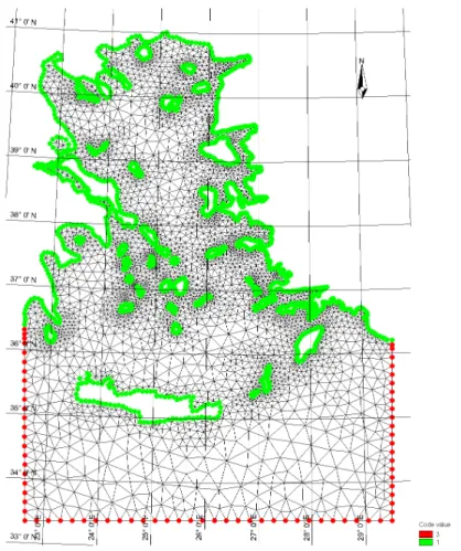
Considering the fact that there is a large number of islands in Aegean Sea and most of them are small and negligible ones from engineering aspect, so that the islands which had less area than the effecting area in this domain were eliminated from the geometry for more efficient computation of the model and making the calculations simpler and faster.
Figure 2.1: Geometry of the Aegean Sea and nodes and vertices used in mesh generation process.
As shown in the Figure 2.1 the domain is located between 33◦N−41◦N and 22◦E−
30◦E, our domain is in UTM-35 zone also nodes in Turkish coastal lines have been taken very close to each other for a smoother mesh generation.
2.2 Boundary Conditions
The boundary condition for the domain in different parts was defined quickly by studying the boundary conditions types in DHI MIKE Mesh Generator Manual. By selecting a number for every boundary it could be very simple for the future steps of the calculations for the program to recognize the boundary type and the process would be without any problems.
For this study there is 2 different type of boundaries:
• Closed Boundary
Figure 2.2: Boundary conditions of the domain.
Each boundary type is defined in mesh generation process and it’s specified in nodes’ attributes, where as “1” means land boundary and values for points and arcs’ attributes that are equal or more than “2” are open boundary conditions.
Boundary conditions which their attribute is specified more than "2" can be later changed in the MIKE 21 SW module. In this case we didn’t have any data on our boundaries to submit to MIKE 21 so that southern boundary of the domain is defined as an open boundary that can pass wave to out of the domain.
As it is shown in Figure 2.2 there are 3 attribute values for arcs available in our domain for which islands are given as “0” as default and defined as land boundaries, Also the coastline of our domain is given as “1” that it means it is land boundary, and the open boundary is given as “2”.
Figure 2.3: General view of unstructured mesh used for the Aegean Sea. Mesh nodes and elements play an important role in computation time and stability of the model. So that this part of the study was conducted with high accuracy to build a high quality mesh to avoid negative consequences in the next levels of the study. Bathymetry data is loaded in Mesh file, and then interpolated by this mesh, also the computations of the wave parameters in the domain will be done with this unstructured mesh. It was tried to produce the best mesh for the study domain.
The meshes generated by the MIKE Zero was not logical in aspect of computation time for numbers of nodes in mesh, sometimes more than 20000 nodes were recommended by the mesh generator, but modifications have taken place to decrease the number of mesh nodes.
Mesh which is used for this thesis consists of 5927 nodes and 10081 elements, the mesh is taken smoother in coastal parts and coarser in offshore to minimize the computation time.
2.4 Bathymetry Data
Bathymetry data of the Aegean Sea was obtained from EMODNet website. This data was determined by ships and other observation instruments and gathered together at this portal, also interpolated with a high resolution. EMODNet portal is user-friendly that the data could be downloaded as many different data file types, like as XYZ, NETCDF, CSV, GEOTIFF, ESRI ASCI, SD file formats.
The main advantage of this website is to obtain the data free of charge and downloading data with more flexible file formats. XYZ file format was chosen for this study because of MIKE Zero compatibility to this file type. The scattered data was applied to mesh by mesh generator module of DHI MIKE.
The resolution of the bathymetric data in this study is 0.004◦. While the domain and the boundaries are defined to MIKE Zero Mesh Generator and interpolation is done, the values out of boundary conditions are excluded.
Also the points which were in the domain was interpolated by the neighboring values and set the value for those points. The data were interpolated by the mesh which was at first generated for the domain and it is obvious that no more data points involved in the calculation for taking more computation time.
Figure 2.4 shows the details of this unstructured mesh which contains mesh nodes and elements, bathymetry and boundary points’ attribute values in Çe¸sme region of Aegean Sea. It can be obviously seen from this figure that the mesh is smoother in the nearshore parts of the domain and coarser in offshore.
Figure 2.5 shows general view of bathymetry while it could be seen in detail when it is zoomed in MIKE ZERO data viewer.
2.5 ECMWF Data
The most important data which is compulsory for the module is wind forcing data to be loaded to program in correct form that could be accepted by MIKE 21. A great effort has been made in this phase to get the data and process to be used efficiently.
2.5.1 ERA-Interim wind data
ERA-Interim data which is the latest global atmospheric reanalysis produced by European Center for Medium-Range Weather Forecasts (ECMWF). The data coverage of this database is from January 1st 1989 until present. This data is measured by satellite every 6 hours in 24 hours, and The best resolution of the data is 0.125◦×0.125◦. ERA-Interim is a large data set which provides other meteorological parameters. In this data set the wind speeds are given for 10 m height from surface in 2 directions.
2.5.2 Preparation of wind data
DFS2 file format is a Grid Series for loading data sets being changed by time. This chapter of the project consisted of these steps:
1. Downloading data files from ECMWF website
2. Changing the format of the GRIB files to CSV format 3. Writing a code for data organization
4. Creating DFS2 file format 5. Loading data in MIKE 21
Data set obtained from ECMWF is called ERA-Interim, that is the most updated and reliable data sets attainable in this field. The values are in U and V surface wind velocity components are presented as matrices that sorted by every time step. The best resolution for the grid is 0.125◦and it was selected for our project.
Data was downloaded for 2 purposes and 2 time periods:
Figure 2.6: Sort of wind speed matrices in 2 directions.
• 1994-1996 (Bozcaada & Dalaman stations)
• 2011 (Athos, E1M3A, Lesvos, Mykonos,Santorini, Saronikos, Skyros stations)
2. Long-time simulation period
• 1999-2013
The data for calibration was downloaded for the area being discussed and reformatted the file from GRIB to Excel format by an open source JAVA program named Panoply. It is essential to first mention properties of the ASCI file in first lines then referring to the values of data for every step. For this aim, Visual Basic is used to custom coding for processing the data more fast and efficiently.
The U and V wind speed components should be sorted in the form shown in Figure 2.6.
Figure 2.7: Visual basic code for cell selection in excel and data organization. direction. Also taking the matrices one from wind speed in x direction and one in y direction respectively for each time step.
For numbering the title of every matrice to set the data into form of the ASCI format the code shown in Figure 2.8 is used.
The last step of DFS2 file preparation is to add the data properties text to ASCI file. A sample ASCI format which is used to define the properties of data and is used in this study is shown in Table 2.3. In this table properties of the DFS2 file is defined.
The last step of the DFS2 file creation is to import the data files which are prepared in TXT file format to be loaded into a Grid Series file in MIKE Zero.
2.6 Measured Data
Measured data is an essential part of the project which is needed to find out the accuracy of the model and to be sure of the results with a high percentage. In this study 9 stations were used to validate model, the locations of each station is shown in Figure 3.1.
Figure 2.8: Visual basic code for building z in excel and data organization. Table 2.3: Format for MIKE DFS2 files.
1 "Title" "File Title" 2 "Dim" 2 3 "Geo" "LONG/LAT" 22 33 0 4 "Time" "EqudistantTimeAxis" "1994-01-01" "00:00:00" 1460 21600 5 "NoGridPoints" 65 65 6 "Spacing" 0.125 0.125 7 "NoStaticItems" 0 8 "NoDynamicItems" 2
9 "Item" "U" "Wind Velocity" "m/s" 10 "Item" "V" "Wind Velocity" "m/s" 11 NoCustomBlocks 0
12 "Delete" -1E-030 13 "DataType" 0
There were 2 different wave parameters needed in this study to be obtained for calibration: 1. Significant Wave Height 2. Mean Wave Period
2.6.1 Buoy data of NATO-TU waves project
This data was measured nearly 10 years ago by a project done by a team members of NATO-TU Waves Project. This project was alive from 1994 to 2000 and was supported by NATO Science for Stability program. The buoys were available in Black Sea, Marmara Sea, Mediterranean Sea and Aegean Sea.
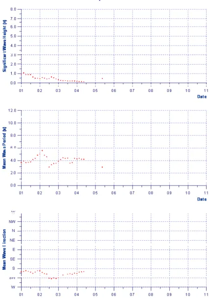
The data which were available from November 1994 to October 1996, free to access on the website of the NATO-TU waves, but the data were plotted on the image format and uploaded on the portal. Also the data were printed as GIF file formats with every 10 days data plot, so that the image processing of the data was a time consuming job. A sample of the data plot of NATO-TU waves is shown in Figure 2.10, where the red dots and lines are the values of the parameter being discussed and the x-axis demonstrates the day of the month. After digitizing every month‘s values then the data were gathered together and a constant value was added to make the days more organized and sorted.
The data attainment was done fast while the data needed to be organized in one file for each parameter, so that 10 days interval data files were attached to each other and has been made a single file of Excel. For further analyses the data was gathered and organized in monthly and yearly periods.
The data was digitized point by point and finding the center of every scatter point to be accurately processed and exported to EXCEL file. A general view of the digitization process is shown in Figure 2.11. The was done by GetDataDigitizer (version 2.26 licensed).
There was 204 plots awaiting to be image processed by hand and it was done completely that the data is ready to be compared with the result of the MIKE 21 test results.
Figure 2.10: Sample image of measured data plotted in GIF file format by NATO-TU Waves.
POSEIDON system which is managed and developed by HCMR is a planning tool for marine protection. This network consists of buoys in Greek coastal and offshore parts which is measuring different wave and marine parameters. The measurements of the data in POSEIDON wave buoy is done with 3 hours interval.
The data source files of this station was obtained in NetCDF file format and converted to excel files to be used easily. The data source for this buoy was obtained from MyOcean website with a monthly period. There are 7 different stations located in study domain.
For every Station, monthly data downloaded and then merged with together with a program named NCO 4.4.4 which is distributed under GNU Free Documentation License, Version 1.3. This program made the whole process more easier to deal with the large number of files of these stations. NCRCAT is an operator of NCO which merges independent data files with common record dimensions into one file.
Table 2.4 shows specifications of different buoys used for calibration in this thesis. The buoy station types used in this study was wave scan Datawell directional wave rider for Dalaman and Bozcaada and multi-parametric deep water Seawatch-Wavescan type for POSEIDON wave buoy.
Table 2.4: Specifications of wave buoys used in calibration. Longitude Latitude Depth Type Athos 24.724 39.973 220 m Wave-Scan Bozcaada 26.0492 39.703 62 m Wave-Scan Dalaman 28.755 36.691 100 m Wave-Scan E1M3A 24.919 35.786 1670 m Wave-Scan Lesvos 25.807 39.156 130 m Sea-watch Mykonos 25.462 37.523 110 m Sea-watch Santorini 25.501 36.262 280 m Sea-watch Saronikos 23.569 37.610 211 m Sea-watch Skyros 24.464 39.113 120 m Sea-watch
3. MODEL VALIDATION
Every model has to be validated with one or series of measured data, to define the model’s reliability. The evaluation of the measured and simulated data could have a great effect on every model’s success degree in estimation of the parameters.
There are many parameters needed for spectral wave model to start the computation, the most important part of this project is to estimate the accuracy of the model, this is not possible without trial and error correction of the parameters to find the best fitting parameters with the results of stations data, this process is called calibration.
3.1 MIKE 21 SW
MIKE 21 SW a new generation spectral wind-wave model is a part of the MIKE program which is developed by Danish Hydraulic Institute (DHI). This program has a high reputation across the wave hydrodynamics researchers and water resources institutes. This model which is based on unstructured meshes simulates growth, decay and transformation of wind generated waves and swell in offshore and coastal regions. There are two main formulation for spectral wave module of MIKE 21:
• Directional decoupled parametric formulation
• Fully spectral formulation
These two formulation are different in the approach to the solution, whereas directional decoupled parametric formulation uses parameterization of the wave action conservation equation, in which the parameterization is done in the frequency domain by introducing the zeroth and first moment of the wave action spectrum as dependent variable [10].
On the other hand fully spectral formulation uses wave action conservation equation which is described in [7] and [32] where the directional-frequency wave action spectrum is the dependent variable.
3.1.1 MIKE 21 SW features
The main features of MIKE 21 SW are as follows:
• Fully spectral or directionally decoupled parametric formulations
• Source functions based on the state-of-art 3rd generation formulations
• Instationary and Quasi-stationary formulation
• Optimal degree of flexibility interpolation of bathymetry with unstructured mesh
• Effects of ice coverage(N/A in this study)
• Extensive range of output parameters
3.2 Definitions
1. Significant Wave Height,Hm0(m);
Hm0=4√m0 (3.1)
2. Maximum wave height,Hmax(m);
The maximum wave heightHmaxis estimated as
Hmax=min(Hmax1 ,Hmin2 ) (3.2) Hmax1 is determined assuming Rayleigh distributed waves
Hmax1 =Hm0 r
1
2Ln(N) (3.3)
where N is the number of waves estimated asN =duration/T01. The duration is set to 3 hours (10800s).H2 is determined assuming monochromatic waves
where α = Ld = 2kdπ, where k is the wave number corresponding to the peak wave period and d is the water depth.
3. Peak period,Tp(s);
Tp= 1 fp
(3.5) The peak frequency fp is calculated from one-dimensional frequency spectrum
using a parabolic fit around the discrete peak. The scheme for computing the peak frequency can be formulated :
• Search through 1D frequency spectrum and obtain the index,ipcorresponding to maximum spectral density.
• Using f0= f(ip−1), f1= f(ip), f2= f(ip+1)and similarly forE0,E1,E2, the peak frequency is given by
fp= f(ip−1)− b 2c (3.6) where b= (f2−f0) 2(E 1−E0)−(f1−f0)2(E2−E0) (f1−f0)(f2−f0)2−(f 1−f0)2(f2−f0) (3.7) c= (f1−f0) 2(E 2−E0)−(f2−f0)2(E1−E0) (f1−f0)(f2−f0)2−(f1−f0)2(f2−f0) (3.8) 4. Mean Period,T01(s); T01= m0 m1 (3.9)
5. Zero crossing period,T02(s);
T02= r
m0
m2 (3.10)
6. Energy averaged mean period,T−10(s);
T−10= 1 ¯ f =
m−1
m0 (3.11)
7. Mean wave direction, ¯θ(degree);
¯
θ =270−tan−1(b
where a and b is defined as: a= 1 m0 Z 2π 0 Z ∞ 0 cos 3 2π−θ E(f,θ)dfdθ (3.13) b= 1 m0 Z 2π 0 Z ∞ 0 sin 3 2π−θ E(f,θ)dfdθ (3.14) 8. Directional standard deviation,σ(degree):
σ = h 2 1−(a2+b2)12 i12 ·180 π (3.15) 9. Particle velocities
The calculation of the horizontal and vertical particle velocity componentsuandw is based on Stokes first order theory for progressive waves, see e.g. [33]:
u(z,φ) =1 2ωH coshk(z+d) sinhkh cosφ (3.16) W(z,φ) = 1 2ωH coshk(z+d) sinhkh sinφ (3.17)
where ω is the cyclic angular frequency, h is wave height, k the wave number, d water depth, z vertical coordinate and φ the phase of the wave. Using the directionally decoupled parametric formulation the root mean square of the maximum value of two components can be calculated as
umax(z) = s Z 2π 0 2ωcoshk(z+d) sinhkh 2 E(θ)dθ (3.18) Wmax(z) = s Z 2π 0 2ωsinhk(z+d) sinhkh 2 E(θ)dθ (3.19) whereE(θ)is wave energy at wave directionθ.
While using the fully spectral formulation the root mean square of the maximum value of the two components can be calculated as:
wmax(z) = s Z 2π 0 Z ∞ 0 2ωsinhk(z+d) sinhkh 2 E(f,θ)dfdθ (3.21) whereE(f,θ)is the wave energy at wave directionθ.
The following values are included in the output:
• Maximum horizontal particle wave velocity at the sea bottom,Umax(z=−d)
• Maximum horizontal particle wave velocity at the free surface,Umax(z=0)
• Maximum vertical particle wave velocity at the free surface,Wmax(z=0)
• Maximum horizontal particle wave velocity at a level,z0,Umax(z=z0)
• Maximum vertical particle wave velocity at a level,z0,Wmax(z=z0)
andz0is defined as:
z0=d+∆d (3.22)
where∆dis user-defined distance above the bed.
10. Wave power;
The energy transport for a harmonic wave is Penergy =ρgcgE in magnitude, where E is the energy density andcg is the group velocity, ρ is the density of water and g is the acceleration of gravity. In random seas the following to definitions of the wave power can be used
• Omni-directional wave power(energy sink)Penergy
Penergy=ρg Z 2π 0 Z ∞ 0 cg(f,θ)E(f,θ)dfdθ (3.23)
• Directional wave power(energy transport)
#
Penergy= (Penergy,x,Penergy,y) (3.24)
# Penergy=ρg Z 2π 0 Z ∞ 0 # cg(f,θ)E(f,θ)dfdθ (3.25) Penergy,x=ρg Z 2π 0 Z ∞ 0 cg(f,θ)cos(θ)E(f,θ)dfdθ (3.26)
Penergy,x=ρg Z 2π 0 Z ∞ 0 cg(f,θ)sin(θ)E(f,θ)dfdθ (3.27) 3.3 Model Parameters
MIKE 21 SW demands different parameters to run the model which is built and described in the Chapter 2 of this thesis. In this Section different model parameters will be discussed and described thoroughly.
The calculation method of MIKE 21 SW module is an important thing to know in the computation process. The computation time and calculations duration is mostly dependent on this approaches.
3.3.1 Source functions
The energy source term, S, represents the superposition of source functions describing various physical phenomena
S=Sin+Snl+Sds+Sbot+Ssur f (3.28) HereSin represents the generation of energy by wind,Snl is the wave energy transfer due non-linear wave-wave interaction, Sds is the dissipation of wave energy due to white-capping,Sbotis the dissipation due to bottom friction andSsur f is the dissipation of wave energy due to depth-induced breaking.
3.3.2 Basic equations
Waves dynamics are dependent on the wave action density. The wave action density is a function of two wave phase parameters. The two wave phase parameters can be the wave number vector #k with magnitude, k, and direction, θ. On the other hand wave phase parameters can also be the wave direction, θ, and either relative angular frequency,
σ =2πfr (3.29)
in the present model the wave direction,θ, and the relative angular frequency,σ, was used. The action density N(σ,θ), is dependent on the energy density E(σ,θ) by Equation 3.31.
N= E
σ (3.31)
Linear dispersion relation is given for the wave propagation over slowly varying depths and currents
σ=pgktanh(kd) =ω−#k ·U# (3.32) in whichgis acceleration of gravity,dis the water depth andU#is the current velocity vector. While magnitude of group velocity, cg, of the wave energy is relative to the current is given by cg=∂ σ ∂k = 1 2 1+ 2kd sinh(2kd) σ k (3.33)
The phase velocity,c, of the wave relative to the current is given by c= σ
k (3.34)
The frequency spectrum is limited to the range between a minimum and maximum frequency, (σmin,σmax). The frequency spectrum is split up into a deterministic
prognostic part for frequencies lower than a cut-off frequency and an analytical diagnostic part for frequencies higher than the cut-off frequency. A dynamic cut-off frequency depending on the local wind speed and the mean frequency is used as in the WAM Cycle 4 model. The deterministic part of the spectrum is determined solving the transport equation for wave action density using numerical methods. Above the cut-off frequency limit of the prognostic region, a parametric tail is applied
E(σ,θ) =E(σmax,θ) σ σmax −m (3.35) where m is a constant. In MIKE 21 SW 2012, m =5 is applied. The maximum prognostic frequency is determined as