A comparative analysis of data mining algorithms to mitigate spurious detections in
Gaia
Author: Esther Pallares Guimera.
Facultat de F´ısica, Universitat de Barcelona, Diagonal 645, 08028 Barcelona, Spain.∗
Advisor: Francesca Figueras
Abstract: Gaia is an ESA mission that observes about 50 million sources per day. A small part of these detections are considered spurious generated for example by cosmic rays. The main objective of this study is to perform a comparative analysis of several algorithms to automatically detect spurious detections. Successfully identifying these detections is important to prevent them from entering the cross-match stage where they create several problems and degrade resolution performance. We will use appropriate metrics to determine the execution and assess the algorithms. Finally, it will be discussed if any of these data mining algorithms could be a good solution to the spurious detection problem.
I. THE GAIA MISSION
Gaia is an European Space Agency (ESA) mission whose main goal is to scan our Galaxy and beyond to build a three dimensional map according to astromet-ric measurements of objects up to magnitude G=20.7. Moreover, photometric and spectroscopic measures are also taken with an unprecedented resolution only possi-ble from space.
It is expected to observe more than a billion stars and solar system objects. Current estimations hint that pro-cessing all these observations will require more than 1021 flops [1].
Gaia has been operating since 2013 and a first version of the catalogue was published on September 2016. The final version is scheduled for 2022. The data is opened to the public and it is expected to make significant contri-butions to the knowledge of our Galaxy, the Milky Way, among other scientific targets.
A. The Gaia Instrument
Gaia has two optical telescopes which correspond to two fields of view (FoV). Both telescopes share the same focal plane depicted in FIG. 1. There are one hundred and six charged couple devices (CCDs) divided into seven rows and into seventeen strips comprising nearly a thou-sand million pixels. A deeper description of the focal plane is detailed in [2].
The Sky Mappers CCDs are in charge of the detection. Point-like sources passing by one telescope are detected. Afterwards, a window is placed around objects of inter-est. Only these windows are read out to reduce back-ground noise. We refer to detections of the Sky Mappers CCDs as detections, observations or transits.
∗Electronic address: [email protected]
Windows pass through one entire row of CCDs, from left to right. The first strip of the astronomic field con-firms the detections made previously on the sky mapper CCDs. Windows pass through two strips of photomet-ric measurements with blue and red bands and, finally radial velocity measures are taken by a radial velocity spectrometer.
FIG. 1: Gaia focal plane scheme. Credit: ESA
B. Spurious Detections
The processing power is limited and so the detection process has to be simple, and sometimes false positives happen, thus producing detections of non-real stars, what we refer to as spurious detections, which can reach up to 20% of all observations for some periods [3].
There are different types of spurious detections: spu-rious detections caused by cosmic rays, by background noise, due to unexpected light paths, as a result of in-ternal reflections within the satellite and around bright sources of magnitude up to 16. We refer to bright sources causing spurious as parent detections. The spurious de-tections are located along the diffraction spikes, but for sources with magnitude brighter than 6, known as Very Bright Sources (VBS), spurious detections appear not
B Spurious Detections Esther Pallares Guimera
only along the diffraction spikes but also in more compli-cated patterns near the bright source.
This work is focused on the classification of spurious detections around bright sources because these are the most frequent spurious type representing around 90% of the total spurious detections. To simplify this work we restricted this initial study to spurious created by sources with magnitudes between G=7.5 and G=12.
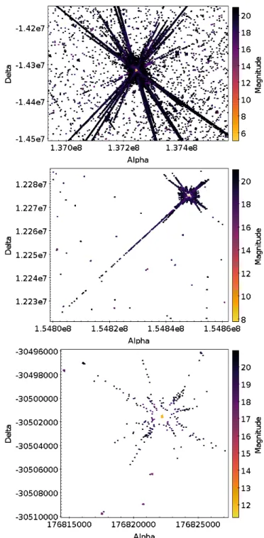
A single transit of a VBS source can produce thousands of spurious detections. A transit of a source of magni-tude G=8 produces hundreds of spurious detections. For sources of magnitude G=12 just a few spurious detec-tions are produced. FIG.2. illustrates the detecdetec-tions of a single transit for a source of magnitude G=5.02 (top), G=8.18 (middle) and G=11.7 (bottom).
II. CLASSIFICATION ALGORITHMS
The two main types of machine learning algorithms are: supervised learning and unsupervised learning. Su-pervised learning algorithms learn from datasets with class known. On the other hand, unsupervised learn-ing algorithms extract their own conclusions from the dataset, but in this case, class is not provided. Unsuper-vised learning algorithms have not been considered as we have several physical information of Gaia detections and we want to control the process.
The aim of a classification algorithm is to choose be-tween a set of options. In this particular case, we intend to decide if an observation belongs to a source or to a spurious. This decision is made according to a model previously created for each algorithm after training it. We have chosen to work with Weka, which provides the implementation for several data mining algorithms [4].
The chosen algorithms for this spurious classification analysis are: REPTree, kstar and IBK, because they ex-ecuted the best performance among others on a first test of magnitude G=8.
A training set is a data set where the classification class of each element is known. The algorithms are trained with this dataset. On the other hand, a test set is a data set where the classification class of each element is unknown. Models are evaluated with test sets. A model is the rule to distinguish an observation between a star and a spurious.
To build the training dataset it was necessary to man-ually classify observations as real or spurious. Thirty-six training sets were generated in total, with a minimum of seven training sets per magnitude between G=7.5 and G=12. In order to do that, Gaia detections were plotted and manually classified using TOPCAT[5].
Defining the dimensionality (number of attributes) of a training set is relevant as machine learning algorithms work better with low rather than high dimensional data sets. For this reason, each attribute has to be relevant. Moreover, if the set of attributes are not relevant the classification will not be performed correctly [6].
FIG. 2: Spurious detections around a source of magnitude G=5.02, G=8.18 and G=11.7 from top to bottom, for several scans. (Units: 10-8rad)
A major part of this study has been to test and refine the necessary parameters for a correct classification. We concluded that absolute attributes (not referenced to any parent observation) such as alpha, delta, magnitude and scan number were not good enough for the classification. For this reason, we decided to reference the attributes to the parent observation.
B Kstar Esther Pallares Guimera
between G=7.5 and G=12. The dataset is created with detections in its surroundings selected with a fix window with different dimensions according to the parent magni-tude.
The final set of attributes chosen per detection has been:
• Parent magnitude: it is a fundamental variable be-cause this magnitude defines spurious distribution complexity around it. A brighter source has more spurious around it as it can be seen in FIG. 2.
• Parent field of view: it allows knowing which tele-scope observed the parent observation.
• Field of view: it informs about which telescope ob-served the detection. This allows algorithms to dis-card detections by FoV if they are not relevant.
• Magnitude difference between the observation and the parent observation: it was selected because spu-rious around bright sources are much fainter than the parent detection.
• AL and AC relative position difference in pixels be-tween an observation and the parent observation: spurious appear in certain patterns, as a result, spurious are more likely to be in a certain region. Therefore, we use these variables to have relative location to the parent observation.
A. REPTree
REPTree is a regression tree algorithm. A tree algo-rithm is based on decision points, named nodes, which are produced by splitting data into smaller subsets. Each data division adds new branches to the tree. Each path from the root to the leaf constitutes a region of data. Each region is fitted with a constant value k.
In regression trees there are three main characteris-tics: splitting rule, termination criterion and assigning a constant value to a terminal node. In this case, REPTree uses information gain (it calculates the expected decrease of entropy) as splitting rule and mean square error as ter-mination rule also known as pruning [7].
B. Kstar
Kstar is a cluster analysis algorithm as well as an in-stance based learner. An inin-stance, x, is assigned to the cluster with the nearest mean measured by entropic dis-tance which has some benefits including handling of real valued attributes and missing values [8].
C. IBK
IBK is an incremental instance-based learning algo-rithm whose leit motiv is: similar instances have similar classification. This type divides training instances de-pending on their category attribute’s value in order to save a set of representative instances, which will allow similarity function and classification function to predict the class of a new instance [9].
III. PERFORMANCE METRICS
In order to compute precision, sensitivity and accuracy we need four numbers: true positives (TP) which means the number of spurious correctly classified as spurious, true negatives (TN) counting the number of sources cor-rectly classified as sources, false positive (FP) meaning the number of sources incorrectly classified as spurious and finally, false negative (FN) meaning the number of spurious incorrectly classified as sources.
We have used the following set of metrics to analyse the performance of the three selected algorithms:
• Execution time: it is the result of building the model from training sets and the classification of a test set.
• Precision: percentage of correctly classified spuri-ous detections out of total, false or not, of predicted as spurious.
P recision= T P
T P +F P (1)
• Sensitivity: percentage of correctly classified spuri-ous detections out of total number of real spurispuri-ous.
Sensitivity= T P
T P+F N (2)
• Accuracy: percentage of correct classification.
Accuracy= T P +T N
T P +T N+F P+F N (3)
Neither precision nor sensitivity depend on the size of the test set, however, accuracy does depend on the number of instances of the test set, but this metric is the most basic measure of the performance of a classifier [10].
In order to validate the classification, two methods have been used, ten fold cross-validation and hold out cross-validation.
Ten fold cross-validation splits the training set in two parts in order to use one of them to compute the model and the other to evaluate it. In our case, data set is divided into ten subsets (nine for training and one for testing).
Hold out cross-validation trains the model with a train-ing set, and tests it with a different dataset [11].
Esther Pallares Guimera
Overfitting is an issue that can happen with these al-gorithms. It occurs when a model reflects excessively a singular training set. The model works perfectly with that training set but it is not trained to be able to cor-rectly perform the classification of a different data set.
The metrics of ten fold cross-validation method were successful with the wrong set of attributes (absolute at-tributes) because the test and training sets used by this method belonged to a unique original set, according to its definition explained before. Thereby, both sets of in-stances, training and test were pretty similar. However, hold out cross-validation showed very bad results due to the model only reflected some specific scenarios.
IV. RESULTS
In order to analyse each algorithm, we started perform-ing a test to determine the minimum number of train-ing sets to obtain good results. We executed the same test several times but increasing the number of training sets. We started to build the model with one training set and each time more independent training sets were concatenated to the initial set, always trying to maintain a proportionality between magnitudes, until the number of spurious stabilized around thirty-eight percent (orange line in FIG. 3). The percentage of spurious detections is the discriminatory parameter, as it is the real number of spurious of our test set. The sum of the numerous independent training sets builds the final training set.
FIG. 3: Graphic evolution for IBK (yellow), REPTree (blue) and kstar (green). The percentage of spurious detections of the input test set of magnitude G=7.77 according to the num-ber of training sets used to build the model.
FIG. 3 shows the percentage of spurious correspond-ing to a test set of magnitude G=7.7. Therefore, if the model behaves correctly in this magnitude, it is expected to behave even better in the rest of magnitudes, due to brighter parents produce more complex spurious detec-tions patterns.
REPTree and kstar show a constant performance from thirty training sets. However, IBK never arrives to con-verge with REPTree and kstar. Hence, the minimum number of training sets has to be bigger than thirty. De-spite this, in theory as more training instances are used to build a model, a better performance is achieved, always avoiding overfitting. Provided that, thirty-six datasets were used to compare the data mining algorithms.
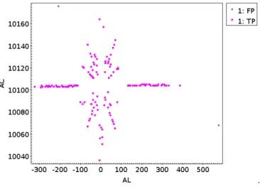
Once we knew the number of training sets, we pro-ceeded to evaluate their performance with ten fold cross-validation and hold out cross-cross-validation, see FIG. 4. The results of these metrics can be seen in TABLE I and II.
Algorithm Precision Sensitivity Accuracy Time (s) REPTree 0,950 0,972 0,979 1,38 kstar 0,765 0,738 0,875 1109 IBK 0,936 0,971 0,976 1,45
TABLE I: Measures of precision, sensitivity, accuracy and execution time with ten fold cross-validation per analysed al-gorithm.
Algorithm Precision Sensitivity Accuracy REPTree 1 0,828 0,932 kstar 0,922 0,888 0,983
IBK 0,400 1 0,588
TABLE II: Measures of precision, sensitivity and accuracy with hold out cross-validation per analysed algorithm.
.
FIG. 4: Classification results with REPTree algorithm of the same test set (G=7.7) FIG. 3 was build. There are two false positives, stars classified as spurious. (Units: pixels)
In this particular case, our training set has more than fourteen hundred instances and the test set has three hundred eighty-nine instances. The necessary time to build the model of an algorithm and perform the classi-fication of a test set is the same for both cross-validation methods.
Esther Pallares Guimera
In table II we can see that some metrics achieve its maximum value, one. In the case of IBK, the sensitivity is maximum because it has over classified data as spu-rious. On the other hand, the precision of REPTree is also maximum because there are not stars classified as spurious.
In table I and II, we can see the difference on IBK precision between ten fold and hold out cross-validation, we assure the degradation in the performance must be due to IBK will require a larger training set. In FIG. 3, IBK do not converge to the expected value, thirty-eight percent. Our assumption is that with IBK the training set still needs more data for a correct training.
Comparing table I and II, REPTree and kstar show some difference between ten fold and hold out cross-validation. In the case of kstar, its metrics are higher in hold out cross-validation, contrary to REPTree. Having into account hold out cross-validation is obtained test-ing an independent test, we will give more weigh to this method.
Table I shows that kstar is much slower than REPTree and IBK. The time difference rose to more than three hours between kstar and REPTree, and it neither had stopped growing nor stabilized with the number of inde-pendent training sets.
V. CONCLUSIONS
It can be said that data mining algorithms are success-fully classifying spurious detections from the Gaia data.
The research of the right set of attributes has taken half of this time work as they are the base for a correct classification. From the first attempts to the final set of attributes has been an evolution, modifying the di-mensionality of the set and adjusting each parameter to
arrive to the final set. In this process, we found out that Gaia data had to be considered by scan instead of multi scan, for example. Moreover, we concluded that increas-ing the trainincreas-ing set size do not improve the performance if the eight attributes are not appropriate. However, the right set of attributes classified much better with a much reduced size training set.
We conclude that REPTree is the best algorithm be-cause its hold out cross-validation metrics are excellent and also its speed. We discard kstar because it is very time consuming, and IBK because executed the worst performance.
As future work, in order to use data mining classifi-cation technique for all Gaia data, the model should be created using training datasets covering the missing mag-nitude ranges G=5 to G=8, and G=12 to G=16. More-over, additional training sets should be manually created and tested for all magnitudes in order to improve the current results. Furthermore, a chance should be given to machine learning algorithms not considered because they might obtain better results with the total range of Very Bright Sources.
Acknowledgments
I would like to thank Nora Garralda and Francesca Figueras for their support and for giving me such an amazing opportunity. This would not have been possible without Gaia Team at the UB, specially Jordi Portell, Juanjo Gonzalez and Marcial Clotet. Finally, I appre-ciate the patience, love and education my parents have given me.
[1] Clotet, M.; Gonzlez-Vidal, J.J.; Casta˜neda, J.; Garralda, N.; Portell, J.; Fabricius, C.; Torra, J.; ”Cross-matching algorithm for the Intermediate Data Updating system in Gaia”; Highlights on Spanish Astrophysics IX (2016). [2] Fabricius, C.; Portell, J.; Casta˜neda, J.; Clotet, M. and
others; ”Gaia data release 1”; Astronomy & Astrophysics (2016)
[3] Garralda, N.; Casta˜neda, J.; Portell, J.; Clotet, M.; Gonzalez-Vidal, J.J.; Torra, J.; ”Treatment of Spurious Detections in Gaia”; Highlights on Spanish Astrophysics IX (2016).
[4] The University of Waikato, URL http://www.cs.waikato.ac.nz/ml/weka/ (2016).
[5] TOPCAT URL http://www.star.bris.ac.uk/ mbt/topcat/ (2016).
[6] Maimon, O.Z.; Rokach, L; ”Data Mining and Knowledge Discovery Handbook”; Springer (2005).
[7] Kalmegh, S; ”Analysis of WEKA Data Mining Algorithm
REPTre, Simple Cart and RandomTree for Classification of Indian News”. International Journal of Innovative Sci-ence. Vol.2 Isuue 2 (2015).
[8] Vijayarani, S.; Muthulakshmi, M.; ”Comparative Analy-sis of Bayes and Lazy Classification Algorithms”. Inter-national Journal of Advanced Research in Computer and Communication Engineering.2: Issue 2 (2013).
[9] Aha, D. W.; Kibler, D.; Albert, M. K.; ”Instance-Based Learning Algorithms”. Department of Information and Computer Science, University of California (1999). [10] Mohapatra, D. P.; Patnaik, S.; ”Intelligent Computing,
Networking, and Informatics”; Proceedings of the Inter-national Conference on Advanced Computing, Network-ing, and Informatics, India (2013).
[11] Liu, L.; Ozsu, M. T.; 2009; ”Encyclopedia of Database Systems”; New York, USA: Springer.