Methods for Analyzing High Dimensional Data with Applications to the Wearable and Microbiome Data Analysis

ScholarWorks at University of Montana

ScholarWorks at University of Montana

Graduate Student Theses, Dissertations, &

Professional Papers Graduate School

2019

Methods for Analyzing High Dimensional Data with Applications

Methods for Analyzing High Dimensional Data with Applications

to the Wearable and Microbiome Data Analysis

to the Wearable and Microbiome Data Analysis

Quy Xuan Cao

Follow this and additional works at: https://scholarworks.umt.edu/etd

Let us know how access to this document benefits you.

Recommended Citation

Recommended Citation

Cao, Quy Xuan, "Methods for Analyzing High Dimensional Data with Applications to the Wearable and Microbiome Data Analysis" (2019). Graduate Student Theses, Dissertations, & Professional Papers. 11507.

https://scholarworks.umt.edu/etd/11507

This Dissertation is brought to you for free and open access by the Graduate School at ScholarWorks at University of Montana. It has been accepted for inclusion in Graduate Student Theses, Dissertations, & Professional Papers by an authorized administrator of ScholarWorks at University of Montana. For more information, please contact [email protected].

Analysis

By Quy Xuan Cao

Dissertation

presented in partial fulfillment of the requirements for the degree of

Doctor of Philosophy in Mathematics The University of Montana

Missoula, MT November 2019

Approved by:

Ashby Kinch, Associate Dean of Graduate School Graduate School

Dr. Ekaterina Smirnova, Chair Mathematical Sciences Dr. Leonid Kalachev Mathematical Sciences Dr. Jonathan Graham Mathematical Sciences Dr. Johnathan Bardsley Mathematical Sciences Dr. Nathan Insel Department of Psychology

All rights reserved

with Applications to the Accelerometry and Microbiome Data

Quy Xuan Cao

University of Montana, 2019

ABSTRACT

Modern studies in medicine, epidemiology, pharmacy and other fields gen-erate high dimensional data. We developed statistical analysis methods for two types of such data: activity and microbiome data. Specifically, reliable mea-sures of the frequency, duration and intensity of physical activity provided by wearable technology were used in the analysis of activity data. Accelerometry-derived measures of physical activity were compared with established predic-tors of 5-year all-cause mortality in older adults, aged between 50 and 85 years from the 2003- 2006 National Health and Nutritional Examination Survey, in terms of individual, relative, and combined predictive performance. A total of 33 predictors of 5-year all-cause mortality, including 20 measures of objective physical activity, were compared using single-predictor and multiple logistic regression. The results show that objective accelerometry-derived physical ac-tivity measures outperform traditional predictors of 5-year mortality in single predictor models, and offer some improvement in multiple predictor models beyond what age and other traditional predictors provide. This highlights the importance of wearable technology for providing reproducible, unbiased, and prognostic biomarkers of health. In microbiome data, we concentrated on pre-processing steps, where both the sparsity of counts and the large number of observed taxa were considered. The current approach is to remove taxa that appear in small counts in a few samples, which is known as filtering. We

designed to address two problems in microbiome data processing: (1) define and quantify loss due to filtering by implementing thresholds; and (2) intro-duce and evaluate a permutation test for filtering loss to provide a measure of excessive filtering. The package employs an unbalanced binary search al-gorithm that greatly reduces computational time for these permutations. The effectiveness of the proposed approach on downstream microbiome data anal-ysis is illustrated on two microbiome quality control datasets. Our filtering method reduces: (1) the magnitude of differences in alpha diversity for samples containing the same bacteria processed at different labs and (2) the dissim-ilarity between samples (beta diversity) that contain the same microbiome potentially alleviating technical variability.

Keywords: High Dimensional, Accelerometry, Physical Activity, Physical Performance, Exercise, Longevity, Microbiome, Filtering, Permutation Test, Binary Search, Skew-normal Distribution, Quality Control.

The completion of this dissertation would not have been possible without the support of those around me. First, I would like to express my deepest gratitude to my advisor, Dr. Ekaterina Smirnova, for her encouragement and essential guidance at every step of the dissertation. Her tremendous help on my research as well as her continued support has led me to the right direction and finish my dissertation. I would also like to extend my appreciation to my committee members: Dr. Jonathan Graham, Dr. Leonid Kalachev, Dr. Johnathan Bardsley, and Dr. Nathan Insel for spending their invaluable time to evaluate my dissertation and provide me with valuable feedback. My sincere appreciation to all the authors who published their papers. They help me enormously in understanding the subject and writing my dissertation.

Finally, I would also like to extend gratitude to my friends and family. Their unfathomable supports during the process helped me achieve my goals.

List of Figures ix

List of Tables xiii

List of Notations xiv

1 Introduction 1

1.1 High dimensional data . . . 1

1.2 Accelerometry data . . . 4

1.3 Microbiome data . . . 7

1.4 Research contributions . . . 10

2 Functional Data Analysis 14 2.1 What is Functional Data? . . . 14

2.1.1 Introduction . . . 14

2.1.2 Basic concepts and notation . . . 17

2.1.3 Summary statistics for functional data . . . 19

2.1.4 Challenges of analyzing functional data . . . 21

2.2 From Discrete to Functional Data . . . 24

2.2.1 Representing Functional Data: Basis Expansions. . . . 25

2.2.3 Choosing the number of basis functions . . . 31

2.3 Principal components analysis for functional data . . . 33

2.3.1 PCA for multivariate data . . . 33

2.3.2 PCA for functional data . . . 36

3 Application of functional data: the NHANES data analysis 40 3.1 Introduction . . . 40

3.2 Study Population . . . 41

3.3 Variables . . . 43

3.3.1 Traditional mortality predictors . . . 43

3.3.2 Accelerometry derived predictors . . . 43

3.3.3 Intuition behind fPCA . . . 48

3.4 Statistical Analysis . . . 53

3.4.1 Mortality prediction models . . . 54

3.5 Results . . . 54

3.6 Discussion . . . 64

4 Microbiome Data Analysis 67 4.1 Microbiome Data . . . 67

4.1.1 Challenge of Microbiome Data . . . 68

4.1.2 The MicroBiome Quality Control data . . . 72

4.1.3 Methodology . . . 75

4.1.4 The PERFect Package . . . 77

4.2 Filtering algorithms . . . 78

4.2.1 Simultaneous filtering. . . 78

4.2.2 Permutation filtering . . . 80 vii

4.3 Application and Evaluation . . . 84 4.3.1 The MicroBiome Quality Control data . . . 85 4.3.2 The reagent and laboratory contamination data . . . . 90 4.3.3 Computation time . . . 94

5 Final Remarks 97

Bibliography 102

A Reference Manual for PERFect software 114

1.1 Publications by year with search terms ‘exercise or physical ac-tivity‘ and ‘accelerometry’. Source: [Troiano et al., 2014]. . . . 3 1.2 Accelerometry data for one subject followed over 5 days. Source:

[Smirnova et al., 2018b]. . . 3 1.3 Raw data summarized as activity counts . . . 5 1.4 Prevalence and abundance of microbial taxa inhabiting healthy

human body sites. Source: [Belizario and Napolitano, 2015] . 8 1.5 Heatmap of 1016 observed taxa on the log-scale, with taxa on

the x-axis arranged in decreasing abundance order and sam-ples on the y-axis arranged by processing institutes. Source: [Sinha et al., 2015] . . . 10 2.1 Canadian average annual weather cycle data. Average monthly

temperature and precipitation at 35 different locations in Canada from 1960 to 1994. . . 15 2.2 Berkeley Growth Study data. Heights of 39 boys and 54 girls

from age 1 to 18 and the ages at which they were collected. . . 16 2.3 Pointwise mean and median functions of the temperature. . . 20 2.4 Sample covariance heatmap of the temperature. . . 21

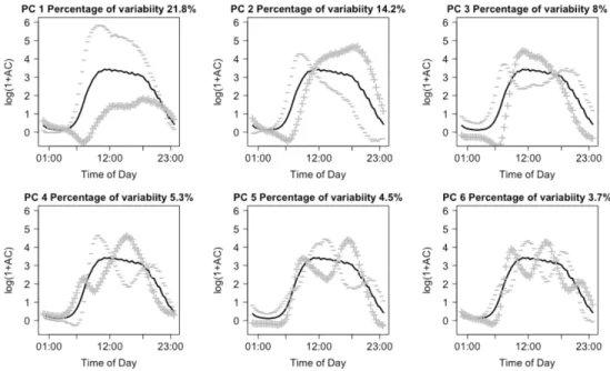
minute level NHANES accelerometry data. Solid lines repre-sent the population average curve; +,- lines denote the effect of being 2 standard deviations from a score of 0 on the particular principal component. . . 47 3.2 Left panel: the first two principal components that explains

the overall variability in the observed daily profiles of activity. The x-axis shows the time of day and the y-axis shows the values of PC curve. Individuals with a positive score on the first PC on a given day will tend to have less activity during the night hours and more activity during the day hours than the average activity across all subject-days. The second PC reflects the contrast between morning and afternoon activity. Right panel: Examples of activity profile for 3 subjects to show the connection between the PCs and the activity profiles. The x-axis shows the time of day and the y-axis shows log(1+AC) values. . . 49 3.3 Left panel: Daily activity profile for subject 21009. Right panel:

Daily activity profile for subject 21039. For both panels, the x-axis shows the time of day and the y-axis shows log(1+AC) values. This figure demonstrates the day-to-day variability of the activity profile for each subject that will influence the PC scores. This shows the importance of the use of means and standard deviations of the PC scores in mortality prediction model. . . 52

added in the forward selection procedure. Predictors are shown on the x-axis, with accelerometry predictors in red. The AIC and EPIC information criterion values are shown on the left y-axis and the AUC values are shown on the right y-axis. This figures shows the best model for each of the three criteria at the colored dots. It also shows the change of AIC, EPIC and AUC as each variable is added into the model. Data source: National Health and Nutritional Examination Survey Pooled Cohorts Study, United States, 2003-2006. . . 60 3.5 Correlation plot between age and accelerometry derived

mea-sures. National Health and Nutritional Examination Survey Pooled Cohorts Study, United States, 2003-2006.. . . 61 4.1 The heatmap of 100 observed taxa on the log-scale, with taxa

on thex-axis arranged in decreasing abundance order and sam-ples on the y-axis arranged by processing institutes. Source: [Sinha et al., 2015] . . . 73 4.2 The multidimensional scaling plot of 1016 samples, colored by

the processing institutes. Source: [Sinha et al., 2015] . . . 74 4.3 DFL and log DFL of MBQC data . . . 80 4.4 Taxa intervals tested by the fast permutation filtering algorithm. 83 4.5 P-values from MBQC data . . . 85 4.6 Alpha Diversity comparison on MBQC data . . . 87 4.7 Multidimensional scaling plots from filtered and unfiltered

MBQC data . . . 89

thex-axis arranged in decreasing abundance order and samples on the y-axis arranged from low to high (0 to 5) degrees of dilution. Source: [Salter et al., 2014] . . . 91 4.9 The multidimensional scaling plots for each degree of dilution,

colored by the processing institutes. Source: [Salter et al., 2014] 92 4.10 Alpha Diversity comparison on salter data . . . 94 4.11 Multidimensional scaling plots from filtered and unfiltered

Salter data. . . 95

3.1 Interpretation of the results of fPCA . . . 53 3.2 Demographic and Clinical Characteristics Separated by Alive

and Deceased Status 5 Years After Participation in the Ac-celerometry Study, National Health and Nutritional Examina-tion Survey Pooled Cohorts Study, United States, 2003-2006. . 58 3.3 Estimated Final Model Coefficients Odds Ratio (OR) with

Cor-responding Standard Errors and Significance Values in the Fi-nal Complex Survey Design Model, NatioFi-nal Health and Nu-tritional Examination Survey Pooled Cohorts Study, United States, 2003-2006 . . . 63 4.1 Major functions in the package PERFect . . . 78 4.2 Summary statistics of the Shannon index for each processing lab. 86 4.3 Pairwise comparisons of the Shannon index. . . 88 4.4 Running time comparison of filtering methods . . . 96

AIC Akaike’s Information Criterion

ASTP Active to Sedentary Transition Probability AUC Area Under the Curve

BMI Body Mass Index

CDC Centers for Disease Control CHD Coronary Heart Disease CHF Congestive Heart Failure CI Confidence Interval

DFL Difference in Filtering Loss

EPIC Efficient Parsimony Information Criterion FDA Functional Data Analysis

FL Filtering Loss

fMRI functional Magnetic Resonance Imaging fPCA functional Principal Component Analysis HMP Human Microbiome Project

ICL Imperial College London

LEfSe Linear Discriminant Analysis Effect Size MBQC MicroBiome Quality Control

MDS Multidimensional Scaling xiv

mi1 Average scores for the first principal component

MSE Mean Squared Error

mV Millivolts

MVPA Moderate/Vigorous Physical Activity

NB Negative Binomial

NRI Net Reclassification Index NDI National Death Index

NGS Next Generation Sequencing

NHANES National Health and Nutrition Examination Survey

OR Odd Ratio

OTU Operational Taxonomic Unit

PA Physical Activity

PC Princial Component

PCA Principal Component Analysis PCR Polymerase Chain Reaction ROC Receiver Operating Characteristic

SATP Sedentary to Active Transition Probability SBP Systolic Blood Pressure

SIBO Small Intestine Bacteria Overgrowth

si6 Standard deviation of the sixth principal component

SN Skew-Normal

TAC Total Activity Count TLAC Total Log Activity Count UB University of Birmingham

ZIG Zero-Inflated Gaussian

ZINB Zero-Inflated Negative Binomial ZIP Zero-Inflated Poisson

Introduction

1.1

High dimensional data

The rise of technological developments has shifted research towards heavier use of computational tools. It began in the late 1960s, when academics started us-ing statistical software like SPSS to perform complex computations instead of manual calculations [SPSS, 2018]. This addition of technology to the research process has reduced the potential for human error and increased computa-tional speed. Several decades later, in the 2000s, the spectacular evolution of data acquisition technologies and computing facilities started changing the way researchers collect and analyze data [Johnstone and Titterington, 2009]. From the classical scenario of ‘small p, large n’ (p is the number of variables

and n is the number of observations), modern data have become ‘large p,

small n’ or ‘large p, large n’, which is now referred to as high dimensional

data. This introduced new complex analyses that include image analysis, ge-nomics research, document classification, and so on. Hence, the need for new data analysis methods to provide computational efficiency and practical results

have increased in response to these changes.

Studies using high dimensional data have shown many significant break-throughs in medicine, epidemiology, pharmacy and other fields. One example of high dimensional data is the activity measure using accelerometry, which has received growing attention in recent years as shown in Figure 1.1. For example, it is extremely difficult for field biologists to track wild animals’ activities; thus their attempts to quantify behavior to model ecological pro-cesses may be inaccurate due to the lack of observing important behavioral events. Using acceleration sensors, researchers can now measure the change in velocity of a body over time as well as quantify fine-scale movements and body postures without issues of visibility, observer bias, or the scale of space use [Brown et al., 2013]. Moreover, the technology and application of current accelerometer-based devices in human physical activity (PA) research allow the capture and storage of large volumes of raw acceleration signal data, which provide opportunities to characterize and improve physical activity behav-ioral patterns [Troiano et al., 2014]. Functional magnetic resonance imaging (fMRI) is another area where high dimensional data arise. Studies in fMRI analyze functional brain networks to better understand how brain regions in-teract, how this depends upon experimental conditions and behavioral mea-sures and how anomalies (disease) can be recognized [Solo et al., 2018]. Lastly, microbiome data are known to be high dimensional due to the number of sam-ples and bacteria identified as a result of the sequencing process. The analyses of the associations between the human microbiome and health aim to under-stand the host-microbiome interactions and integrate them with other ‘omics’ datasets to enhance precision medicine [Petrosino, 2018].

Figure 1.1: Publications by year with search terms ‘exercise or physical activ-ity‘ and ‘accelerometry’. Source: [Troiano et al., 2014].

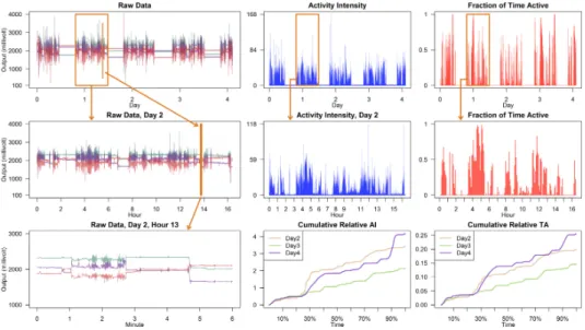
Figure 1.2: Accelerometry data for one subject followed over 5 days. Source: [Smirnova et al., 2018b].

1.2

Accelerometry data

In this dissertation, two types of high dimensional data are considered for analysis: accelerometry data and microbiome data. Figure 1.2 displays ac-celerometry data collected at a frequency of 10 Hz for five days from a sensor placed on the hip of a person [Bai et al., 2012]. The top left panel shows data measured along three orthogonal axes (up-down, left-right, backward-forward in the device frame of reference) for one subject, whose data consist of ap-proximately 13 million observations. The five days of long periods of higher amplitude signals are separated by four nights characterized by low amplitude signals. To get a closer view, the box in the top-left panel in Figure 1.2 which identifies day 2 of the data is zoomed in as shown in the left-middle panel. A vertical line indicates a period of six minutes during day 2, which is further zoomed in and shown in the left-bottom panel. As one looks at finer resolu-tions of the data, more patterns can be identified and possibly used. These raw data are expressed in millivolts (mV), though most devices output raw data in Earth gravitational units (g = 9.81m/s2_{). Working directly with raw}

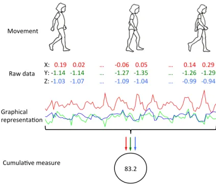
data could be quite daunting and, in practice, data are often summarized as activity counts (or steps) per minute as in Figure1.3, resulting in a matrix of

n×1440, wherenis the number of samples and 1440 represents the number of

minutes per day. The middle-top panel in Figure1.2 provides such a summary measure at the minute level, while the middle-center panel displays the same measure for day 2. While informative, overlaying such visualizations in the same panel will lead to over-plotting and loss of information when comparing different days or subjects or when displaying an entire cohort. Instead, the middle-bottom plot shows the cumulative measure of activity up to a

partic-ular time of the day. This panel contains exactly the same information as the middle-center panel, but allows for joint plotting of multiple days and sub-jects. The right panels display similar information, although they focus on the proportion of time active per minute instead of activity intensity during that minute. The proportion of time active is obtained by calculating the activity intensity at the second level, applying a threshold on activity intensity that indicates active/inactive, and then computing the proportion of active seconds within that minute [Smirnova et al., 2018b] [Karas et al., 2019].

0 10 20 30 40 50 60 70 80 90 100 -0.8 -0.6 -0.4 -0.2 0 0.2 0.4 0.6 0.8 X: 0.19 0.02 … -0.06 0.05 … 0.14 0.29 Y: -1.14 -1.14 … -1.27 -1.35 … -1.26 -1.29 Z: -1.03 -1.07 … -1.09 -1.04 … -0.99 -0.94 83.2 Movement Raw data Graphical representaFon CumulaFve measure

Figure 1.3: Raw data summarized as activity counts

Traditionally, the physical activity data resulting from accelerometry mea-sures are analyzed using methods in functional data analysis (FDA), which

deals with data that are in the form of continuous functions [Augustin et al., 2017], [Smirnova et al., 2019] and [Leroux et al., 2019]. Here, each function is typically observed at a finite number of points, and in the case of accelerometry data summarized at the minute level, these functional data are observed throughout 1440 points (minutes) in a day. Key aspects of FDA include the choice of smoothing technique, dimension reduction, adjustment for clustering and functional linear modeling [Finch, 2013]. The first step in any FDA is smoothing, which represents raw discrete data points as a smooth function that emphasizes patterns in the data by minimizing noise due to observational errors. In particular, the use of B-spline basis functions is one of the most popular smoothing techniques [Aguilera and Aguilera-Morillo, 2013]. As for data reduction, functional principal components analysis (fCPA) is a popular multivariate analysis technique for extracting information from mul-tiple variables by reducing the dimensions of a dataset while preserving as much of the total variation as possible [Croux and Ruiz-Gazen, 2005]. As fPCA results in dimension reduction, fPCA vector scores can be used for clustering different functions/components using standard clustering methods [Finch, 2013]. In the accelerometry data context, clustering helps to identify representative curve patterns and individuals with similar activity patterns. An interesting application of FDA involves the construction of functional lin-ear models that describe the relationship between a response and explanatory variables [Usset et al., 2016]. Here, functions could be used as the response variable, the predictors or both. In R, the package fda [Ramsay et al., 2018] and refund [Goldsmith et al., 2018] provide various statistical tools for func-tional data analysis and are freely available for researchers to use.

1.3

Microbiome data

Microbiome data are another type of high dimensional data that will be dis-cussed in this dissertation. To generate a microbiome dataset, the first step is to collect samples which could be taken at various body sites [Belizario and Napolitano, 2015], as shown in Figure 1.4. These samples are sequenced using the next generation sequencing (NGS) of the 16S ribosomal RNA genes technology to generate DNA fragments, which are then grouped into similar microbial organisms called taxa [Sanschagrin and Yergeau, 2014]. The resulting dataset, which has samples in the rows and taxa in the columns, is a large sparse matrix as many rare taxa are identified. In current mi-crobiome studies, the goal is to understand mechanisms of host genetic and environmental factors that shape the microbiome. For example, in 2008, a multi-institutional collaboration called the Human Microbiome Project (HMP) was established to generate resources that facilitate characterization of the hu-man microbiota and further our understanding of how the microbiome impacts human health and disease [Turnbaugh et al., 2007]. Specifically, this project aimed to develop a reference set of 3,000 isolate microbial genome sequences, understand the ‘core’ microbiome at five regions in the body (nasal passages, oral cavity, skin, gastrointestinal tract, and urogenital tract), determine the relationship between disease and changes in the human microbiome and de-velop new tools and technologies for computational analysis [HMP, 2008]. However, it is difficult to reproduce studies across labs because variation in measurements between laboratories has not been systematically assessed. The Microbiome Quality Control (MBQC) project was therefore initiated to iden-tify sources of variation in microbiome studies, to quaniden-tify their magnitudes,

and to assess the design and utility of different positive and negative control strategies [Sinha et al., 2015].

Figure 1.4: Prevalence and abundance of microbial taxa inhabiting healthy human body sites. Source: [Belizario and Napolitano, 2015]

Dynamic interactions exist among environment, microbiome and host. For microbiome studies, the focus is to test the association between the microbiome and the host, specifically whether the composition of the mi-crobiome or ‘dysbiotic’ mimi-crobiome is linked to the health or disease of the host [Xia and Sun, 2017]. For example, in small intestine bacteria overgrowth (SIBO) research, dysbiosis is associated with the overgrowth of pathogenic bacteria in the small intestine, causing pain and diarrhea and leading to malnutrition [Leite et al., 2019]. It is also of interest to test whether the microbiome is associated with environmental covariates or whether there is

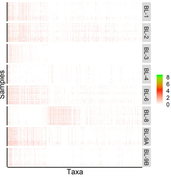
an effect of intervention of a specific microbiome composition on health and disease [Chen et al., 2012]. Examples include testing whether dietary inter-ventions shape gut microbiota [Albenberg et al., 2012] and understanding the impact of a probiotic intervention on the composition of the human microbiota [Lahti et al., 2013]. However, when analyzing microbiome data, taxa counts are often overdispersed and have many zeros as displayed in Figure 1.5. In order to fit microbiome count data with overdispersion and excess zeros, the negative binomial (NB) [Zhang et al., 2018] and zero inflated models such as the Zero-Inflated Poisson (ZIP), Zero-Inflated Negative Binomial (ZINB) and Zero-inflated Gaussian (ZIG) mixture model [Paulson et al., 2017] were chosen for modeling the excess zeros and testing differential abundance taxa between groups.

Figure 1.5: Heatmap of 1016 observed taxa on the log-scale, with taxa on the x-axis arranged in decreasing abundance order and samples on the y-axis arranged by processing institutes. Source: [Sinha et al., 2015]

1.4

Research contributions

The research problems studied as part of this dissertation, include the anal-ysis of the National Health and Nutrition Examination Survey (NHANES)

accelerometry data as well as the development of methodology for the micro-biome quality control problem. Specifically, the accelerometry data studies have mainly focused on developing interpretable metrics for summarizing raw tri-axial accelerometry data [Bai et al., 2013] [Bai et al., 2016], deriving ap-propriate measures for physical activity [Varma et al., 2018] and re-evaluating the effect of age on physical activity over a lifespan [Varma et al., 2017]. How-ever, development of mortality predictive models using accelerometry data and the influence of physical activity while considering traditional predictors such as age and body mass index simultaneously remained open. Hence, for my research, I explored the associations between participants’ physical activity, demographic and health-related characteristics and 5-year all-cause mortality in NHANES data, performed single-predictor logistic regression to identify the ranking of the most predictive predictors and their relative effects on mortality, and compared derived measures of physical activity to established predictors of 5-year all-cause mortality. With the assistance of my collaborators from Johns Hopkins University in deriving information criterion for complex sur-vey design model, I was able to build a multiple logistic regression model using forward selection. Our results led to two publications and were fea-tured in the recent press release of the Johns Hopkins University [JHU, 2019]. Moreover, I contributed to the R package rnhanesdata (available on github) which organizes and helps with the analysis of the Activity Data in NHANES [Leroux et al., 2019]. In this package, I helped with automating the extraction of data from the Centers for Disease Control and Prevention website, merging multiple files into one final file and cleaning the data based on our exclusion criteria. A detailed vignette that describes the data processing steps and anal-ysis is publicly available within the package to guide researchers who plan to

use this package and replicate our findings.

For microbiome data, the microbiome quality control problem needs to be addressed prior to data analysis. Recent microbiome quality control stud-ies show that the majority of rare taxa are caused by contamination and/or sequencing errors [Sinha et al., 2015]. The most common approach to ad-dress this problem is to filter spurious taxa from the data, and one of the most widely used techniques for filtering in microbiome studies is to select taxa that have a number of counts above m = 0 in at least n samples.

[Davis et al., 2018] introduced the decontam R package that identifies con-taminants using DNA concentration information which might not be always available. [Smirnova et al., 2018a] introduced a filtering test, PERFect, by filtering out taxa with insignificant contribution to the total covariance. How-ever, the earlier software implementation was computationally intensive due to the complex permutation filtering algorithm. Hence, using the idea of an unbalanced binary search algorithm, I developed a fast implementation of this algorithm that optimally finds the set of taxa to be removed without building the permutation distribution and computing the p-values for all taxa [Morin, 2013]. The proposed approach successfully reduces the algorithm run time by almost four times. I also developed the R package PERFect which was published in Bioconductor, a free and open development software project for the analysis and comprehension of genomic data [PERFect, 2019]. The reference manual for this package can be found in the appendix of the dis-sertation. I then evaluated the effect of filtering on two major exploratory analyses used in microbiome research: alpha and beta diversity. The meth-ods were applied to two data sets, namely the MicroBiome Quality Control (MBQC) project from [Sinha et al., 2015] and the laboratory contamination

dataset from [Salter et al., 2014]. Results show that the filtering methods re-duce the magnitude of differences in alpha diversity for samples containing same bacteria processed at different labs. Filtering further reduces dissim-ilarity between samples (beta diversity) that contain the same microbiome and potentially alleviates technical variability. Results of this research are currently being prepared for publication.

The rest of the dissertation is organized as follows. I introduce the neces-sary background for functional data in Chapter 2. I show in Chapter 3 the application of functional data analysis in the NHANES data. The microbiome data and the filtering method PERFect are described in Chapter4. Conclud-ing remarks follow in Chapter 5.

Functional Data Analysis

2.1

What is Functional Data?

2.1.1

Introduction

Functional data analysis corresponds to analysis of information on continuous functions (or curves), typically observed at a finite number of points. The primary interest is to study the behavior of such data, and their relationship to other quantities. For example, Figure2.1displays average monthly temper-ature and precipitation data at 35 different locations in Canada averaged over 1960 to 1994 [Ramsay and Silverman, 2006]; each smoothed curve can be con-sidered as a function of temperature and precipitation of each location over time. Another example from [Ramsay and Silverman, 2006] is the Berkeley growth study data, displayed in Figure 2.2, in which the heights of boys and girls were recorded from age 1 to 18. Here, heights of boys and girls can be treated as smoothed functions over the 18 recorded ages.

Figure 2.1: Canadian average annual weather cycle data. Average monthly temperature and precipitation at 35 different locations in Canada from 1960 to 1994.

Figure 2.2: Berkeley Growth Study data. Heights of 39 boys and 54 girls from age 1 to 18 and the ages at which they were collected.

From both examples, temperature, precipitation and height govern the be-havior of functional variables which are of interest in functional data analysis. By definition, a functional variable is a random process X(t) with t taking

values in a closed interval [tmin, tmax], such that for each fixed t0, X(t0) is a random variable. This is the underlying ‘smooth’ process that generates the data we observe. In other words, since the data are assumed to have been generated from an underlying random process, the set of observations {X(t1), ..., X(tm)} is considered as a single curve observed at m grid points.

This is the main difference between functional and longitudinal data, since in longitudinal analysis we do not assume that such an underlying random pro-cess generated the data but instead an m−dimensional vector with a specific

correlation structure. A simple example of such a process is X(t) = a0+a1t

wherea0 anda1 are independently and identically distributedN(0,1) random

variable with a mean and a variance (both are functions of t0). Moreover, for

any two valuest1 and t2, X(t1) and X(t2) are correlated and their covariance

function is defined asK(t1, t2) = Cov{X(t1), X(t2)}.

For each random process, it is possible to have multiple measurements but no parametric assumptions are typically made on the underlying process. The primary interest is to describe the variation of the underlying process. For example, we may ask what feature separates the temperature curves and pre-cipitation curves, how can we discriminate the temperature patterns between Montreal and Resolute, how can we predict a boy’s height using girl growth curves, and are growth spurt (rate of change) patterns different for boys and girls.

2.1.2

Basic concepts and notation

In this section, we review some of the essential concepts that define functional data. For simplicity, these concepts will be listed out as follows.

Definition 1 (Derivatives and integrals): Given a function f(t), denote

the mth derivative by f(m)(t) = Dmf = dm_dtfm(t). Also the integral of f will be denoted by R

f =R

f(t)dt.

Definition 2 (Function space): A set of functions which have a particular property in common. For example, the space of all real-valued square inte-grable functions defined on [0,1], i.e. L2_{[0,1] space.}

Definition 3 (Inner product and norm): For two functions f(t) and g(t)

(belonging to the same function space L2_{), the inner product is defined as:}

hf, gi=

Z

Given the definition above, the norm of a function is given by:

kfk=hf, fi1/2 ₌ Z _f2_(t)dt1/2_,

which satisfies the three important properties of a norm: 1. kfk ≥ 0 and kfk = 0 if and only if f = 0

2. kafk= akfk for any real number a

3. kf+gk ≤ kfk+kgk (Triangle Inequality).

Typically, the norm of a function measures its size and how far from zero the function is in the function space to which it belongs.

Definition 4 (Distance between two functions): The distance between two functions f and g is defined as:

d(f, g) =kf −gk,

which is symmetric and non-negative since it is based on a norm.

Definition 5 (Orthogonality): Two functions f and g are called orthogonal if hf, gi= 0.

Defintion 6 (Basis expansion of a function): A basis function system for a function space is a set of known (possibly infinitely many) functions φk, k=

1,2, ... such that any functionf can be written as a linear combination of the

basis functions, i.e.:

f(t) =

∞

X

k=1

akφk(t),

where ak, k ≥1 are real numbers known as the coefficients of basis

2.1.3

Summary statistics for functional data

Suppose we observe n functional observations X1(t), ..., Xn(t) observed on

[0,1]. The sample mean function is defined as the point-wise average of the

observed functions, given by

¯ X(t) = 1 n n X i=1 Xi(t),

and the sample median function is defined as the point-wise median of the observed functions, given by

¯

Xm(t) = Med{Xi(t), i= 1, ..., n}.

The sample variance function is then naturally derived as

VarX(t) = 1 n−1 n X i=1 {Xi(t)−X¯(t)}2,

and the standard deviation function is the square-root of the variance function. Moreover, the covariance function, which characterizes the underlying process that generates the data, is defined as

CovX(s, t) = 1 n−1 n X i=1 {Xi(s)−X¯(s)}{Xi(t)−X¯(t)} = 1 n−1Xc T_X c,

whereXcis the centered matrixXthat contains discrete observations of these

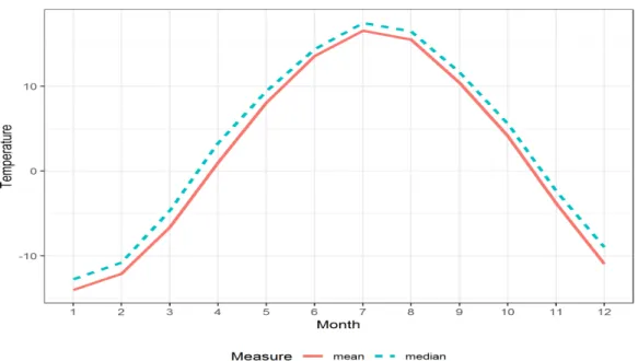
n functions. Figure 2.3 shows a sample mean and a sample median and

func-tion using the temperature data at 35 different locafunc-tions in Canada. Since the median function is higher than the mean function, this is the temperature

distribution is slightly right-skewed. Figure 2.4 shows a corresponding sample covariance function for these locations. For example, CovX(1,2) is the

covari-ance of the temperature in 35 locations between January and February. This covariance function has lower covariance toward the center of the heatmap and higher covariance in four corners of the heatmap, indicating that there are more variability of temperature in winter months than summer months.

Figure 2.4: Sample covariance heatmap of the temperature.

2.1.4

Challenges of analyzing functional data

When analyzing functional data, we are interested in identifying the features that characterize the functions. Some features may be obvious, such as the sinusoidal shape of the temperature functions in Figure2.1, but there may be others that are hidden within. Since each function can be considered as an element of an infinite dimensional function space with infinitely many bases, ideally we want to represent each function using only finitely many bases. One approach to accomplish this is the Principal Component Analysis (PCA), which reduces the dimension of the data while explaining a significant percent of variability present in the data. Specifically, given ap×pcovariance matrix,

we seek eigenvectors u1, ...,up such that

Σ = λ1u1uT1 +...+λpupuTp,

where λ1 ≥ λ2 ≥ ... ≥ λp > 0 are eigenvalues, and the eigenvectors form an

orthonormal basis system. Given the data vectors X1, ...,Xn, the principal

component scores corresponding to the first component are given by

P C1i =uT1Xi=hu1,Xii, i= 1, ..., n,

and the scores corresponding to the other components are defined similarly. The basic idea of functional PCA is similar. Since the functions are assumed to be generated from an underlying process X(t), we start with the

covari-ance function of this process, K(s, t) = Cov{X(s), X(t)}. Thus we seek an

eigenfunction decomposition of this covariance function:

K(s, t) =

∞

X

k=1

λkψk(s)ψk(t),

where φk(·), k ≥ 1 are called eigenfunctions, which are known as ‘modes of

variation’, describing a certain percent of variation in the data. These eigen-functions are denoted as harmonics. Hence, the principal component scores are defined for the first harmonic as:

ξ1i =hψ1, Xi−X¯i=

Z

ψ1(t){Xi(t)−X¯(t)}dt,

and the scores corresponding to the other components are defined similarly. Later in this chapter, we will discuss in more detail the functional Principal

Component Analysis and apply it extensively in our data analysis.

Predictive models can also be built with functional data. For example, to find out if there is any relationship between the total amount of precipitation of a location and its monthly temperature profile, we can perform functional linear regression with a scalar response and functional covariate. Specifically, letZi, i= 1, ...,35 be the total precipitation at the ith location, and letXi(t),

t = 1, ...,12 be the monthly temperature profile. Then the regression model

has the form:

Zi =α+

Z 12

1

Xi(t)β(t)dt+i,

where α is an unknown intercept, β(·) is an unknown regression coefficient

function and i is the error term for each location.

In a different setting, if we want to predict the daily precipitation profile of a location based on its daily temperature profile, we can also fit a functional linear model with a functional response, which has the form:

Zi(t) = α(t) +

Z 365

0

Xi(s)β(s, t)ds+i(t),

where Zi(t) is the precipitation at time t, Xi(t) is the temperature at time

t, α(t) is an unknown intercept function that describes the overall day-to-day

change in precipitation regardless of temperature,i(t) is a random error

pro-cess, and β(s, t) is the unknown regression surface, the relative weight placed

on the temperature at day s, for s= 1, ...,365 to predict the precipitation at

2.2

From Discrete to Functional Data

Recall that the philosophy of functional data analysis is to think of observed data functions as single entities, rather than merely as a sequence of individual observations. In practice, functional data are usually observed and recorded discretely as n pairs (tj, Yj), where Yj is a snapshot of the function at time

tj, with possible measurement errors. Therefore, it is crucial to uncover the

underlying function for each set of observed discrete data. In this section, we will discuss methods for transforming raw discrete data into smooth func-tions using linear combinafunc-tions of basis funcfunc-tions. Indeed, representing data recorded at discrete times as a smooth function would allow us to evaluate the function at any time point, which is extremely useful if we want to compare subjects that were observed at different time points, and examine the rates of change for each underlying curve, given that it is smooth (having one or more derivatives).

In general, observed functional data are recorded as {(Yij;tij) : j =

1, ..., mi}i, for 1 ≤i≤n, whereYij is the snapshot of the underlying function

at time tij for subject i, possibly blurred by error, tij varies in a continuum

interval τ and may not be the same across subjects and ij is the error

as-sociated with recording Yij. The underlying ith function, which is assumed

smooth on τ is denoted as Xi and these Xi’s are independent realizations of

a stochastic process X. In practice, Yij is assumed to be a measure of Xi at

2.2.1

Representing Functional Data: Basis Expansions

The goal of basis expansion is to choose a set of bases so that their span includes good approximations of most smooth functions. Since they have to represent the underlying structure in the sample data, they must be able to flexibly exhibit the required curvature where needed, but also to be nearly linear when appropriate. Furthermore, for computational reasons they should be computationally efficient, easy to evaluate, and differentiable as often as required.

A generic underlying function Xi has the form

Xi(t) =ci1φ1(t) +ci2φ2(t) +...+ciKφK(t)

= Φ(t)ci,

where Φ(t) = (φ1(t), . . . , φK(t)) are predefined basic functions for Xi and

ci = (ci1, . . . , ciK)T are coefficients associated with Φ(t). Here, a basis function

system is defined as a set of known functionsφk that are mathematically

inde-pendent of each other and have the property that any function can be approxi-mated arbitrarily well by taking a weighted sum or linear combination of a suffi-ciently large numberKof these basis functions [Ramsay and Silverman, 2006]. In the example above, we say that{φk, k = 1,2, ..., K}is a basis system forXi.

Since we assume Yij =Xi(tij) +ij from above, each ‘snapshot’ of a function

Yi at time tij can be estimated as

Yi(tij) =Xi(tij) +ij, j = 1, . . . , mi

≈ci1φ1(tij) +ci2φ2(tij) +...+ciKφK(tij) +ij.

in order to achieve a good approximation using a small number K of basis

functions. Hence, we want to choose an appropriate basis system that only requires a small number of bases to fit the data. Besides reflecting certain char-acteristics of the data, the small K is more computationally efficient, yields

more degrees of freedom for hypothesis testing and confidence intervals, and potentially gives meaningful coefficients that can become interesting descrip-tors of the data.

For the rest of this section2.2.1, we will discuss three basis function systems that are widely used in practice and when to use them. To summarize what follows, although a Monomial basis works well with very simple problems, most functional data analyses employ either a Fourier basis for periodic data or a B-spline basis for non-periodic data. Specifically, B-spline bases will be discussed in detail since they are used in the “Application of functional data: the NHANES data analysis” chapter.

Monomial Basis

Polynomials are perhaps the oldest and best known basis function expansion. They can be considered as the senior citizens of the basis world since they can only deal with the simplest functional problems. A polynomial function X(t)

has the form

X(t) =

K

X

k=1

cktk−1,

where tk_{, k = 1, . . . , K are the basis functions, i.e. they are the}

monomi-als{1, t, t2_{, t}3_{, . . . , t}K−1_{} and c}

k are the corresponding coefficients. For simple

problems (which usually occur when the function X(t) is smooth),

localized features, and can run into computational problems for unequally spaced data. Derivative estimation is another limitation of polynomials be-cause their derivatives get simpler as the order of derivative increases, whereas in most real world systems, derivatives become more complex as the order of derivative increases.

Fourier Basis

The Fourier basis system contains basis functions that are sines and cosines of increased frequency:

{1,sin(ωt),cos(ωt),sin(2ωt),cos(2ωt), ...,sin(kωt),cos(kωt), ..}.

This basis is periodic, and the parameterωdetermines the period of oscillation

P = 2π/ω. The number of bases needed is then K = 2M+ 1, where M is the

largest number of oscillations required in a period of length P.

The Fourier series is a familiar concept to statisticians, engineers and ap-plied mathematicians that possesses a lot of advantages when apap-plied in func-tional data representation. The Fourier basis functions have excellent com-putational efficiency, especially if the times of observations are equally spaced due to the orthogonality property of the basis [Ramsay and Silverman, 2006]. It can be shown that if the number of observations is a power of 2 and the arguments are equally spaced, the Fast Fourier transform allows us to find all the coefficients extremely efficiently [Tolimieri et al., 1989]. In terms of fit-ting data, they are natural for describing periodic data such as the Canadian weather example in Figure 2.1. Their derivatives are also simple to calculate since the derivative of a Fourier series expansion is also a Fourier series expan-sion, making the Fourier series infinitely differentiable. However, if the data

are known to have discontinuities in the function or in the derivatives, the Fourier series become inappropriate.

B-Spline Basis

Spline functions are the most common choice of approximation system for non-periodic functional data. To define a spline, we first divide the interval over which a function is to be approximated intoLsub-intervals, separated by

‘knots’ (breakpoints). Over each sub-interval, a polynomial of order m, which

is the number of constants required in the polynomial (one more than its degree), is fitted and joined with other polynomials from adjacent intervals. Thus, a spline is a piece-wise function made of polynomial segments joined end-to-end such that adjacent polynomials join up smoothly at the knots and are thus differentiable at these points. The number of parameters required to fit a spline function is the order plus the number of interior knots,m+ (L−1),

which is also the total degrees of freedom. Moreover, derivatives up to order

m−2 must also match up at these junctions. For example, for the commonly

used order four cubic spline, the second derivative is a line and the third derivative is a step function.

Given the definition of a spline function, we can now construct a system of basis spline functions φk(t) which comprise a B-Spline basis. Each basis

function φk(t) is a spline function defined by an order m of the polynomial

segments and the location of the knots. Specifically, a spline function S(t)

combination of K =m+ (L−1) basis functions: S(t) = m+L−1 X k=1 ckφk(t, τ),

where φk(t, τ) is the B-Spline basis function defined by the knot sequence τ,

evaluated at t and ck is the associated coefficient. Although there are many

ways that such systems can be constructed, [Ramsay and Silverman, 2006] chooses the B-spline basis system developed by [de Boor, 2001], which is the most popular since it allows fast computation for thousands of basis functions and has the flexibility to fit any polynomial of order m. In general, the order

of the spline should be at least m + 2 if we are interested in m continuous

derivatives. The most common choice for polynomial order is m = 4 (cubic

function), implying continuous second derivatives which are linear functions. Moreover, knots are often equally spaced by default such that each interval contains at least one data point, but it is recommended to place more knots where the function exhibits the most complex variation, and fewer where the function is only mildly nonlinear.

2.2.2

Smoothing Functional Data: Least Squares

Once a basis system is chosen, the natural next step is to quantify the quality of the approximation of the functional data. The classical solution for this prob-lem is least squares estimation, a method that minimizes the sum of squared errors between the observed data and the fitted data. Specifically, let us con-sider a set of observations{(Yj, tj) :j = 1, ..., m}and assumeYj =X(tj) +j,

with noise j. We want to estimate X(t) = K X k=1 ckφk(t) =cTΦ(t), wherecT _{= (c}

1, ..., cK)T is the row vector of lengthKof coefficients and Φ(t) =

(φ1(t), ..., φK(t)) is the column vector of length K containing basis functions.

Let Φ be the m×K matrix obtained by row-stacking Φ(tj) for j = 1, ..., m

andY= (Y1, ..., Ym)T. The ordinary least square (OLS) criterion assumes that

residuals are independently and identically normal with mean 0 and variance

σ2_{, i.e:} j

iid

∼ N(0, σ2_{). Given that this assumption is appropriate for the}

data, we can determine the coefficients of the expansion cT = (c1, ..., cK)T by

minimizing SSE(c) = m X j=1 {Yj −X(tj)}2 = m X j=1 {Yj −cTΦ(tj)}2 = (Y−Φc)T(Y−Φc).

After taking the derivative of SSE(c) with respect to c and solving, the OLS estimate of c is therefore

ˆ

c= (ΦTΦ)−1ΦTY,

and the fitted value at time tj is

ˆ

X(tj) = Φ(tj)ˆc

In practice, the independently and identically distributed residual assumption of OLS may not be met. For example, the data may be uncorrelated but exhibit heteroskedastiscity (non constant variance). In such situations, we weight the observations by extending the least squares criterion to the weighted least squares (WLS) form: W M SE(c) = m X j=1 wj{Yj −X(tj)}2 = m X j=1 wj{Yj −cTΦ(tj)}2 = (Y−Φc)TW(Y−Φc),

where W is a diagonal matrix with the diagonal elements equal to wj. It is

usually estimated by the covariance matrixΣ of Y asW=Σ−1, where since

the Yj are uncorrelated (cor(Yi, Yj) = 0 for i 6= j), the off-diagonal terms of Σ are zeroes. The weighted least squares estimate ˆc of the coefficient vector

c is then

ˆ

c= (ΦTWΦ)−1ΦWY

and the fitted curve at point tj is calculated as

ˆ

X(tj) = Φ(tj)(ΦTWΦ)−1ΦWY, j = 1, ..., m.

2.2.3

Choosing the number of basis functions

During the data fitting process, the more basis functions we select, the better the fit to the data but the higher the risk of fitting noise or variation that we do not need. Although the bias would be small, the sampling variance would be large, similar to the over-fitting problem in linear regression. Nevertheless, if

we do not choose enough basis functions, we may miss some important aspects of the function that we are trying to capture, potentially resulting in large bias. Hence, the mean squared error is often used as a loss function that controls the bias and variance of the estimator of the curve. Specifically, for a fixed t,

the mean squared error (MSE) in estimating X(t) is defined as

M SE{Xˆ(t)}=E[{Xˆ(t)−X(t)}2]

= Bias2{Xˆ(t)}+ Var{Xˆ(t)},

where the bias of the estimator is

Bias{Xˆ(t)}=X(t)−E{Xˆ(t)}

and the corresponding sampling variance is

Var{Xˆ(t)}=E[{Xˆ(t)−E[ ˆX(t)]}2_].

The optimal number of basis functions K to fit a curve would minimize the

integrated mean squared error

M SE( ˆX) =

Z

τ

M SE{Xˆ(t)}dt,

which can be be approximated numerically by _m1 Pm

j=1M SE{Xˆ(tj)}when the

2.3

Principal components analysis for

func-tional data

After the preliminary steps of registering and displaying the data, we want to explore the data to see the features characterizing typical functions. Some of these features can be detected easily, such as the sinusoidal nature of the temperature curves, but other features might be more obscure. Principal com-ponents analysis (PCA) of functional data is then a key technique to identify these hidden features. In fact, it is the first method to be considered in the early literature of functional data analysis since it provides us a way to examine the variance-covariance and correlation functions that can be very informative. In this section, we will briefly review the classical principal components anal-ysis for multivariate data and then introduce its version for functional data.

2.3.1

PCA for multivariate data

One of the problems with multivariate data is that there are simply too many variables to make the application of graphical techniques successful in provid-ing an informative initial assessment of the data. Moreover, havprovid-ing too many variables can also cause problems, such as multicollinearity, for other multi-variate techniques that the researcher may want to apply to the data. Principal components analysis is a multivariate technique with the central aim of reduc-ing the dimensionality of a multivariate data set while accountreduc-ing for as much of the original variation as possible. This aim is achieved by creating a new set of variables, the principal components, that are linear combinations of the original variables, which are uncorrelated and are ordered so that the first few

of them account for most of the variation in all the original variables. Ideally, the result of a principal components analysis would be the creation of a small number of new variables that can be used as surrogates for the originally large number of variables and consequently provide a simpler basis for graphing or summarising the data, and for further multivariate analyses of the data.

Let the data matrixXbe of sizen×p, wherenis the number of samples and

pis the number of variables. Let us also assume that each variable is centered,

i.e. column means have been subtracted and the centered means are now equal to zero. Principal components analysis describes variation in a set of correlated variables, xT _{= (x}

1, ..., xp)T, in terms of a new set of uncorrelated variables,

yT _{= (y}

1, ..., yp)T, each of which is a linear combination of thexvariables. The

new variables are derived in decreasing order of ‘importance’ in the sense that

y1accounts for as much of the variation as possible in the original data amongst

all linear combinations of x. Then y2 is chosen to account for as much of the

remaining variation as possible, subject to being uncorrelated with y1, and so

on. The new variables defined by this process, y1, ..., yp, are the orthogonal

principal components. The general hope of principal components analysis is that the first few components will account for a substantial proportion of the variation in the original variables, x1, ..., xp, and can be used to provide a

convenient lower-dimensional summary of these variables.

Finding the principal components

The first principal component of the observations,y1, is the linear combination

whose sample variance is greatest among all such linear combinations. Since the variance ofy1 could be increased without limit simply by increasing the

co-efficients ψT

1 = (ψ11, ψ12, ..., ψ1p)T, a normalization restriction must be placed

on these coefficients: the sum of squares of the coefficients should take the value 1. Hence, to find the coefficients defining the first principal component, we need to choose the elements of the vector ψ1 that maximize the variance

of y1, subject to the constraint ψ1Tψ1 = 1. The second principal component,

y2, is defined to be the linear combination

y2 =ψ21x1+ψ22x2+...+ψ2pxp

that has the greatest variance subject to the following two conditions: ψ₂Tψ2 = 1 and ψT

2ψ1 = 0, i.e. y1 and y2 are uncorrelated. Continuing in this fashion, the jth _{principal component is that linear combination y}

j =ψjTxthat has the

greatest variance subject to the conditions ψT

j ψj = 1 and ψjTψi = 0 for all

i < j. To calculate each ψj, we solve the eigenequation

Σψj =λjψj,

where Σ is the sample variance-covariance matrix which is defined as Σ =

N−1_XT_{X (X is the centered data matrix),ψ}

j is thejth eigenvector ofΣwith

the corresponding eigenvalue λj. Putting all eigenvectors as columns of a

ma-trix V and corresponding eigenvalues as entries of a diagonal matrix Λ, the above equation can be extended to ΣV =VΛ, or Σ=VΛVT, the eigen de-composition ofΣ. Here, the columns of Vare called the principal components (PCs) which are orthogonal with unit norm; Λ is a diagonal matrix, defined

as Λ = diag{λ1, λ2, . . . , λp} where the entries are non-negative and arranged

in decreasing order. The entry λk, k = 1, . . . , p gives the variance of the data

along the corresponding PC and the proportion of variance explained by the

kth _{PC is defined as λ}

k/Ppl=1λl. Finally, the projections of the data on the

principal components are known as PC scores; these can be seen as new trans-formed variables. The jth principal component projection is given by the jth

column ofXV and the coordinates of the ith data point in the new PC space are given by the ith row of XV.

2.3.2

PCA for functional data

Functional principal components analysis (fPCA) was first developed by C. Radhakrishna Rao in 1958 [Rao, 1958]. It is used to analyze the geometry of the functions, capture the principal modes of variation and reduce the di-mension of the data. Let X1(t), . . . , Xn(t) denote independent and identically

distributed random functions on a compact interval T such that each func-tion Xi(t) belongs to the functional space of all real valued square integrable

functions defined on [T], i.e. the L2[T] space, with the true mean function

defined asµ(t) =E[Xi(t)] and their corresponding covariance function defined

as Σ(s, t) = Cov{Xi(s), Xi(t)}. For simplicity, let us assume that the functions

are observed fully on T and without noise.

Similar to PCA, fPCA is based on finding principal component scores of maximum variance that highlight features of the smooth underlying curves. Specifically, to find the first functional principal component, we find the prin-cipal component weight function (eigenfunction) ψ1(t) for which the set of

values

ξ1i =

Z

T ψ1(t)Xi(t)dt

=hψ1, Xii i= 1, . . . , n

has the largest variance, subject to the constraint hψ1, ψ1i = 1. The second

functional principal component finds the eigenfunction ψ2(t) for which the set

of values

ξ2i =

Z

T ψ2(t)Xi(t)dt

=hψ2, Xii i= 1, . . . , n

has the largest variance, subject to the constraint hψ2, ψ2i= 1 and hψ1, ψ2i=

0. Continuing in this fashion, the kth _{functional principal component score}

finds the eigenfunction ψk(t) for which the set of values

ξki =

Z

T ψk(t)Xi(t)dt

=hψk, Xii i= 1, . . . , n

(2.1)

has the largest variance, subject to the constrainthψk, ψki= 1 andhψk, ψji= 0

for all j < k.

In order to calculate the eigenfunctions {ψk(t), k = 1, . . . , n} and

rep-resent any given function X(t) in terms of these eigenfunctions, we use

the theories from Mercer’s theorem and the Karhunen-Lo`eve expansion [Happ and Greven, 2015]. Mercer’s theorem allows for the eigen-decomposition of a covariance function Σ(s, t) into eigenvalues λk and eigenfunctions ψk(t).

intervalT and square integrable, Mercer’s theorem states that there exists an orthonomal sequence ψk of continuous functions inL2[T] with unit norm and

a non-increasing sequence of positive numbersλ1 ≥λ2 ≥... >0 such that

Σ(s, t) =

∞

X

k=1

λkψk(s)ψk(t) s, t ∈ T,

with the eigenvalues and eigenfunctions being solutions to

Z

T Σ(s, t)ψk(s)ds=λkψk(t).

A complete proof of this theorem can be found in [Bosq, 2000]. When Mercer’s theorem holds, the Karhunen-Lo`eve theorem states that using the basis func-tions determined by the eigenfuncfunc-tions of the covariance function, the curves

Xi have the following representation

Xi(t) = µ(t) +

∞

X

k=1

ξikψk(t),

where the basis coefficients are the principal component scores ξik defined

similarly as in equation 2.1:

ξik =

Z

T{ψk(t)(Xi(t)−µ(t))}dt

(2.2)

such that ξik ∼N(0, λk) and they are uncorrelated for differentk. Recall that

we are interested in finding the set of K orthogonal functions {ψ1, . . . , ψk}

functions, then the mean integrated squared error (MISE) criterion M ISE= n X i=1 ||Xi−Xˆi||2 = n X i=1 Z T{Xi(t)− ˆ Xi(t)}2dt (2.3)

is minimized. [Ramsay and Silverman, 2006] show that the set of basis func-tions that minimizes equation2.3has the additional property that it maximizes the amount of variation explained in the random functions Xi(t). Hence, the

collection of the first K eigenfunctions in the sample of curves {Xi(t), i =

1, . . . , n} forms a set of basis functions that minimizes the above MISE

cri-terion. Since these basis functions are derived directly from the functional data instead of being chosen like the Fourier or B-spline basis, they can be considered as empirical basis functions.

Application of functional data:

the NHANES data analysis

3.1

Introduction

The National Health and Nutrition Examination Survey (NHANES) is a cross-sectional, nationally representative survey designed to evaluate the health and nutritional status of adults and children in the United States [CDC, 2016]. The survey samples around 5000 non-institutionalized civilians annually to represent the US population. In particular, NHANES oversamples underrep-resented groups, including elderly people 60+ years old, African Americans, Asians, and Hispanics. The survey involves a 4-stage process to sample par-ticipants, which indicates that the sample is not a simple random sample from the US population. To make the sample representative for the US population each individual sampled in the NHANES has a survey weight, which is defined as the number of individuals in the US population represented by that individ-ual. These survey weights need to be incorporated in any analysis to ensure