Complex-Valued Neural Networks: Learning Algorithms and Applications

(1)

Complex-Valued Neural Networks:

Learning Algorithms and Applications

Md. Faijul Amin

Department of System Design Engineering University of Fukui

A dissertation submitted to the University of Fukui for the degree of Doctor of Engineering

(2)

(3)

This is to certify that the thesis entitled “Complex-Valued Neural Networks: Learn-ing Algorithms and Applications” is approved for the degree of Doctor of EngineerLearn-ing.

Prof. Hiroshi Ikeda, Member

Prof. Yoichiro Maeda, Member

Prof. Kazuyuki Murase, Supervisor

Prof. Tomohide Naniwa, Member

(4)

(5)

Abstract

Complex-valued data arise in various applications, such as radar and ar-ray signal processing, magnetic resonance imaging, communication systems, and processing data in the frequency domain. To deal with such data prop-erly, neural networks are extended to the complex domain, referred to as complex-valued neural networks (CVNNs), allowing the network parame-ters to be complex numbers and the computations to follow the complex algebraic rules. Unlike the real-valued case, the nonlinear functions in the CVNNs do not have standard complex derivatives as the Cauchy-Riemann equations do not hold for them. Consequently, the traditional approach for deriving learning algorithms reformulates the problem in the real domain which is often tedious. In this thesis, we first develop a systematic and simpler approach using Wirtinger calculus to derive the learning algorithms in the CVNNs. It is shown that adopting three steps: (i) computing a pair of derivatives in the conjugate coordinate system, (ii) using coordinate transformation between real and conjugate coordinates, and (iii) organiz-ing derivative computations through functional dependency graph greatly simplify the derivations. To illustrate, a gradient descent and Levenberg-Marquardt algorithms are considered.

Although a single-layered network, referred to as functional link network (FLN), has been widely used in the real domain because of its simplicity and faster processing, no such study exists in the complex domain. In the FLN, the nonlinearity is endowed in the input layer by constructing linearly independent basis functions in addition to the original variables. We design a parsimonious complex-valued FLN (CFLN) using orthogonal least squares (OLS) method, where the basis functions are multivariate polynomial terms. It is observed that the OLS based CFLN yields simple structure with favorable performance comparing to the multilayer CVNNs in several applications.

It is well known and interesting that a complex-valued neuron can solve several nonlinearly separable problems, including the XOR, parity-n, and symmetry detection problems, which a real-valued neuron cannot. With this motivation, we perform an empirical study of classification performance of single-layered CVNNs on several real-world benchmark classification prob-lems with two new activation functions. The experimental results exhibit that the classification performances of single-layered CVNNs are compara-ble to those of multilayer real-valued neural networks. Further enhancement of discrimination ability has been obtained using the ensemble approach.

(6)

(7)

I dedicate this dissertation to my parents

(8)

First and foremost, I thank the Almighty for giving me the strength and ability to complete this study.

I express my deep sense of appreciation, reverence, and sincere gratitude to my supervisor, Prof. Kazuyuki Murase, for introducing me this promising research area. I am indebted to him for his unlimited encouragements, proper guidance, and invaluable advices throughout this work. I would like to thank the committee members of my doctoral exam, who carefully read this thesis and corrected my mistakes.

My sincere appreciation goes to Dr. Md. Monirul Islam who introduced me neural networks for the first time, taught me a great deal about this field, and gave me invaluable suggestions.

It is my eldest brother, Muhammad Harunur Rashid, who has guided me from my childhood and has been a source of inspiration throughout my life. I could never be at my current position without his care and affection. I am grateful to the Japanese Government for the financial support I re-ceived from the Ministry of Education, Culture, Sports, Science and Tech-nology (MEXT).

I express my sincere thanks to all my laboratory members for their con-stant supports and encouragements. Special thanks to Muhammad Aminul Haque Akhand and Takaki Kiritoshi for their kind assistance to adjust life in Japan.

I am greatly indebted to my parents and my wife for their supports and sacrifices throughout my life. My daughter, Fareefta Zaeema, was born during this course of study and it was the most joyful event in my life. Last but not the least, I wish to express my gratitude to all those who have one way or another helped me in making this study a success.

(9)

List of Figures

1.1 Artificial neural network. . . 1 1.2 Left, amplitude and right, phase of land surface (Mount Etna, Sicily,

Italy) obtained by an InSAR system. Image taken fromhttp://epsilon. nought.de/tutorials/insar_tmr/img40.htm . . . 3 1.3 Magnitude of acquired signalS(k) ink−space and its Fourier transform

(spin densityρ(r)) in position space. Note from Eq. (1.1) that S(k) is the inverse Fourier transform of ρ(r). The image has been taken from http://www.scopeonline.co.uk/pages/tutorials/kspace6.shtml . 4 1.4 (a) I/Q signal modulation in passband and bandpass channel with

addi-tive white Gaussian noise (AWGN),w(t), followed by I/Q demodulation. (b) Equivalent complex baseband representation, where ˜m(t), ˜v(t), ˜h(t), and ˜w(t) denote the complex baseband representations for bandpass sig-nals, mbp(t), vbp(t), hbp(t), and complex AWGN, respectively. Channel impulse responses in passband and complex baseband are related by

hbp(t) =<{h˜(t)2ej2πfct}, where<{·}represents the real part. . . 5 1.5 (a) Original image ‘boat’. (b) Original image ‘eline’. (c) Synthesized

im-age by taking magnitude of ‘boat’ and phase of ‘elaine’. (d) Synthesized image by taking magnitude of ‘elaine’ and phase of ‘boat’. . . 6 1.6 Hand tree representation by complex number. After preprocessing by

image processing techniques the segments construct a tree, each having a length and angle. . . 7

(14)

2.1 A neuron with input signalx= (x1, x2, . . . , xm)T, connection weightw= (w1, w2, . . . , wm)T, and bias θ. The linear part combines the weighted sum yielding neuron’s internal state callednet-input. The Nonlinear part transforms the net-input by an activation function f to produce outputy. 14 2.2 Activation functions in real-valued neurons: (a) log-sigmoid, (b)

hy-perbolic tangent, (c) and (d) log-sigmoid and hyhy-perbolic tangent, re-spectively, with amplitude A = 2 and different gain coefficients c =

{0.5,1.0,3.0_}. . . 15 2.3 Complex-valued function f(z) = 1/(1 +e−z_{), where}_z₌_x₊_jy_{. (a) real}

part, (b) imaginary part, (c) amplitude, and (d) phase of the function. . 17 2.4 Real-imaginary-type complex activation function: (a) real part, (b)

imag-inary part, (c) amplitude, and (d) phase of the function. . . 21 2.5 Amplitude-phase-type complex activation function: (a) real part, (b)

imaginary part, (c) amplitude, and (d) phase of the function. . . 22

3.1 Functional dependency graph of a single hidden layer CVNN correspond-ing to Eq. (3.13). Each node represents a complex-vector-valued vari-able, and an edge connecting two nodes is labeled with the Jacobian of its right node with respect to its left node. (a) The general case, acti-vation functions are nonholomorphic and (b) the special case, actiacti-vation functions are holomorphic. In the holomorphic case, conjugate Jacobians are the zero matrix. Thus, graph (a) reduces to graph (b). . . 32 3.2 Learning curves of complex gradient descent, complex-LM, and

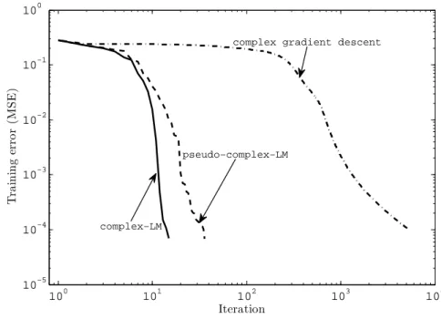
pseudo-complex-LM algorithm. . . 39

4.1 Schematic of functional link network (FLN). The original N input vari-ables are expanded byM linearly independent functions and the output is their linear combination. . . 44 4.2 (a) The best monomials is the one having the smallest angle withd. (b)

The monomials generally are correlated because of nonorthogonality. . . 50 4.3 (Prediction performance: (a) actual and one step ahead prediction of

wind speed by CFLN and (b) actual and one step ahead prediction of wind speed by ACLMS. . . 61 4.4 Symbol error rates at different SNR levels. . . 63

(15)

LIST OF FIGURES

5.1 Class distribution by CVN model of Nemoto and Kono(47) in the net-input or the neuron’s internal state space. Net-input inside the circle of radius h is assigned class label ‘0’ and outside the circle class ‘1’ is assigned. . . 68 5.2 Discrete states of CVN model of Aigenberg et al (1). The CVN takes

n= 8 states according to Eq. (5.2). Each state is one of then₋th roots of unity on the complex plane. States enclosed in the square designates one class and the others denote the opposite class. . . 71 5.3 Orthogonal decision boundaries in the net-input space of a CVN,

pro-duced by the real and imaginary part of its net-input. Combination of two boundaries produces four regions. Two regions (black circles) des-ignate one class, while the remaining two regions (white circles) denote the opposite class. . . 73 5.4 Phase encoded inputs. When a real variable x moves in the interval

[a, b], the corresponding complex variable moves over the upper half of unit circle. x=aand x=b are mapped intoei0 _{= 1 and}_eiπ₌₋_{1 and} respectively. . . 74 5.5 The proposed activation functions 1 and 2 that map complex number

z=u+ivinto real numbers y. (a) Activation function 1 is the magni-tude of sigmoided real and imaginary parts,_|f_R(u) +if_R(v)_|. (b) Acti-vation function 2 is the square of differences between sigmoided real and imaginary parts, (f_R(u)₋f_R(v))2. . . 77 5.6 Net-inputs of a CVN for XOR problem and contour diagram for

activa-tion funcactiva-tions 1 and 2 in (a) and (b), respectively. Curved lines indicate the points taking the same output values as indicated by the numbers. Cross mark [_×] denotes the net-input for the input pattern belonging to class 1 (target output 1), and circle [O] denotes the net-input be-longing to class 0 (target output 0). In each figure, thick curve shows discriminating contour threshold. . . 81 5.7 Net-inputs of a single CVN for sixteen possible input patterns for the

four-input symmetry detection problem on the contour diagrams of (a) activation function 1, and (b) activation function 2. In each figure, thick curve shows discriminating contour threshold. . . 84

(16)

5.8 Basic mechanism of ensemble construction. Dashed rectangle shows an optional step. . . 91 5.9 Bagging algorithm for creating ensemble of single-layered CVNN. . . 95

(17)

List of Tables

3.1 Learning patterns. . . 38

4.1 Input-output mapping of XOR problem with cross product term. . . 45 4.2 Selection of monomials in CFLN for function approximation of Eq.(4.11) 58 4.3 Performance comparison among CRBF, C-ELM, FC-RBF, FLANN, RFLN,

and the proposed CFLN for the function given by Eq.(4.11). . . 59 4.4 Prediction performance of CFLN and ACLMS . . . 60 4.5 Performance comparison among CRBF, C-ELM, FC-RBF, FLANN, RFLN,

and the proposed CFLN for nonlinear channel equalization. . . 62

5.1 Complex-valued encoding of XOR problem . . . 72 5.2 Input-output mapping for XOR problem after phase encoding of inputs. 80 5.3 Input-output mapping of a symmetry detection problem with three

in-puts. Output 1 means corresponding input pattern is symmetric, and 0 means asymmetric. . . 83 5.4 Number of parameters for single-layered CVNNs and two-layered RVNNs.

Parameters include the connection weights and the biases of the neurons. For CVNN, each weight and bias are counted as two parameters, since they have real and imaginary parts. . . 87 5.5 Total number of examples and partitioning of the datasets into training,

validation, and test sets. . . 87 5.6 Average classification error on the test set, and the average number of

epochs required to reach the minimum validation error. Averages are taken over 20 independent runs. Act. 1 and 2 refer to activation function 1 and activation function 2, respectively. . . 89

(18)

5.7 Average number of epochs required to reach the minimum validation error for the phase encoding [0, π/2] and [0, π]. Averages were taken over 20 independent runs. . . 90 5.8 Input-output relationship of three-bit parity problem and the outputs of

three CVNs. The rightmost column shows the averages of the outputs. . 94 5.9 Characteristics of data sets and number of epochs. . . 97 5.10 Average test set error rates (percentage of misclassifications on unseen

data) of single-layered CVNNs and their ensembles trained with negative correlation learning algorithm. Averages were taken over five standard 10-fold cross-validations. The rightmost column shows percentage of error reduction by the ensemble with respect to a CVNN’s error. . . 99 5.11 Average test set error rates (percentage of misclassifications on unseen

data) of single-layered CVNNs and their ensembles trained with bag-ging algorithm. Averages were taken over five standard 10-fold cross-validations. The rightmost column shows percentage of error reduction by the ensemble with respect to a CVNN’s error. . . 100 5.12 Test set error rates of RVNN (having one hidden layer) ensembles and

single-layered CVNN ensembles for two ensemble methods, NCL and bagging. . . 102

(19)

Chapter 1

Introduction

Artificial Neural networks (ANNs) are by far the most commonly used connectionist model today, aiming to solve the problem of learning and design of intelligent machines. Structurally, they are interconnected networks of simple information processing units called neurons as shown in Fig. 1.1. These models are motivated from the biological neural networks and the way information processing takes place therein. Some essential features that make ANNs useful and attractive are mentioned below.

Input #1 Input #2 Input #3 Input #4 Output Hidden layer Input layer Output layer

Figure 1.1: Artificial neural network.

• Nonlinearity: Since the underlying mechanism for generating signal (e.g., speech)

in many physical system is nonlinear, it is highly desirable for system model to be nonlinear. Nonlinearity in ANNs is achieved in a distributed manner by the transfer functions of individual neurons.

(20)

• Learning input-output mapping: An ANN learns input-output relationship from given examples or data set using some supervised learning mechanism. The mapping learned then can be used to infer about new instances not encountered before. This ability is known as generalization. It is observed that the ANNs have excellent generalization ability (5). Unlike many statistical methods, ANNs provide nonparametric inferences in the sense that no assumptions are made with the distribution of input data.

• Adaptivity: Knowledge is represented in the ANNs in the form of connection

(synaptic) weights much like biological neural networks. ANNs have a built-in capability to adapt their synaptic weights to changes in the surrounding envi-ronment. This remarkable ability has resulted popular deployment of ANNs in adaptive pattern recognition, adaptive signal processing, and adaptive control.

• Fault toleranceAn ANN implemented in hardware has a potential to be fault

tolerant, in the sense that its performance degrade gracefully even if some con-nections or neurons are damaged.

The fundamental difference between ANNs and classical information-processing models is that the latter requires formulating a precise mathematical model from obser-vations, whereas ANNs are based on the principle,let the data speak for itself, thereby build implicit model of the environment. In other words, the desirable properties in learning machines are inherently included in the ANNs.

1.1 Why Complex-Valued Neural Networks?

Having introduced with the ANNs and their advantages, it is now time to highlight on title of the thesis which naturally raises a question in one’s mind: why do we need complex-valued neural networks (CVNNs)? This section attempts to answer this ques-tion with some examples.

Although most of the research efforts in neural networks have been focused on the realm of real numbers, they are not the all we know about the number system. Real numbers are just a subset of a more general set called complex numbers. It should be emphasized here that complex numbers are not merely a mathematical abstract. They do exist and arise in many practical considerations. Some examples are given below.

(21)

1.1 Why Complex-Valued Neural Networks?

• Radar signals: Recently, interference of electromagnetic waves is utilized in the

interferometric synthetic aperture radar (InSAR) to obtain complex-valued image of an object. A transmitter emits a microwave signal and a receiver measures the reflected wave in a phase-sensitive way, by mixing the signal wave with a reference wave and observing their interference. Generally, the amplitude represents the reflectance of object and phase represents its distance. For example, Fig. 1.2 shows a complex-valued image of the Mt. Etna, Sicily, Italy taken by an InSAR system. Left part is called amplitude interferogram and the right part as phase interferogram (in modulo 2π). Such a complex-valued image is used for land segmentation (23), construction of digital elevation model(22), and to monitor earthquake(40).

Figure 1.2: Left, amplitude and right, phase of land surface (Mount Etna, Sicily, Italy) ob-tained by an InSAR system. Image taken fromhttp://epsilon.nought.de/tutorials/ insar_tmr/img40.htm

• Magnetic resonance imaging (MRI): In the MRI, magnetic properties of

atomic nuclei are used to visualize human tissue and brain activities (functional MRI). External magnetic field causes the nuclei to produce a rotating magnetic field detectable by the scanner. While the objective is to estimate spin density

ρ(r) over 2D or 3D spacer, actual signal measurements,S(k), are taken in the so calledk−space that defines spatial frequencies. The relation betweenS(k) ink−

space and spin densityρ(r) in position space is given by the Fourier transform as shown below.

S(k) = Z

(22)

Slice in k space S(k)

Slice in position space ρ(r)

Fourier Transform

Figure 1.3: Magnitude of acquired signal S(k) in k₋space and its Fourier transform (spin densityρ(r)) in position space. Note from Eq. (1.1) thatS(k) is the inverse Fourier transform of ρ(r). The image has been taken from http://www.scopeonline.co.uk/ pages/tutorials/kspace6.shtml

As the Eq. (1.1) shows, acquired signalS(k) is essentially complex-valued. Fig-ure 1.3 shows the magnitude in k₋space and magnitude of its Fourier transform position space. Although traditional approaches discard the phase values, re-cent researches have shown much better processing by including phase to form complex-valued signals (11).

• Complex baseband representation of bandpass signal: Almost every

com-munication system operates by modulating an information bearing waveform onto a sinusoidal carrier whose frequency varies over different physical transmission method. The carrier frequency of the transmitted signal, however, is not the component which contains the information. Consequently, communication sys-tem engineers often use a complex baseband representation of communication signals to simplify their job. Figure 1.4 shows a communication system model and its equivalent complex based band representation. In phase and quadra-ture phase (I/Q) signals, mI(t) and mQ(t), are modulated with a carrier to produce a passband signal s(t), which then pass through a wideband channel,

hbp(t). At the receiver end I/Q demodulation takes place resulting the signals,

vI(t) and vQ(t). As shown in Fig. 1.4, a convenient complex based represen-tation is given by ˜m(t) = mI(t) +jmQ(t) and ˜v(t) = vI(t) +jvQ(t), while the

(23)

1.1 Why Complex-Valued Neural Networks? ˜ w(t) vQ(t) vI(t)

×

+

hbp(t) w(t)

+

LPF LPF

~

sin(2πfct) cos(2πfct) − − ˜ h(t) (a) (b) I/Q demodulation Wideband channel

×

~

I/Q modulation mI(t) mQ(t) sin(2πfct) cos(2πfct) mbp(t) vbp(t) ˜ v(t) =vI(t) +jvQ(t) vbp(t) ˜ m(t) =mI(t) +jmQ(t)

Figure 1.4: (a) I/Q signal modulation in passband and bandpass channel with addi-tive white Gaussian noise (AWGN),w(t), followed by I/Q demodulation. (b) Equivalent complex baseband representation, where ˜m(t), ˜v(t), ˜h(t), and ˜w(t) denote the complex baseband representations for bandpass signals,mbp(t),vbp(t),hbp(t), and complex AWGN,

respectively. Channel impulse responses in passband and complex baseband are related by hbp(t) =<{˜h(t)2ej2πfct}, where<{·}represents the real part.

(24)

channel impulse responses in passband and complex baseband are related by

hbp(t) =<{h˜(t)2ej2πfct}. Here<{·}represents the real part.

(a) (b)

(c) (d)

Figure 1.5: (a) Original image ‘boat’. (b) Original image ‘eline’. (c) Synthesized image by taking magnitude of ‘boat’ and phase of ‘elaine’. (d) Synthesized image by taking magnitude of ‘elaine’ and phase of ‘boat’.

• Importance of phase in image processing: Real-valued signals like image

and audio are often analyzed in the frequency domain involving complex numbers. Then the original real-valued signals are characterized by magnitude and phase spectrum in the frequency domain. In the case of image signals, a fundamental result showing the importance of phase was illustrated by (52). It was shown that the information about edges and shapes are contained in the phase, whereas the magnitude contains the information of contrast and contribution of certain frequencies. For an illustration purpose, we took an experiment with two different images, ‘boat’ and ‘elaine’. Each image was transformed into frequency domain by 2D Fourier transform, and then the phases were exchanged keeping the magnitude

(25)

1.1 Why Complex-Valued Neural Networks?

same as the original images. Figure 1.5 shows the synthesized images obtained by the 2D inverse Fourier transform. Although the magnitude spectrum of image in Figure 1.5(c) is same as ‘boat’, it looks much like as ‘elaine’ because its phase spectrum was taken from the original ‘elaine’ image. Similar phenomena can be observed in Figure 1.5(d). This clearly demonstrates that proper treatment in signal processing can be done using complex-valued data.

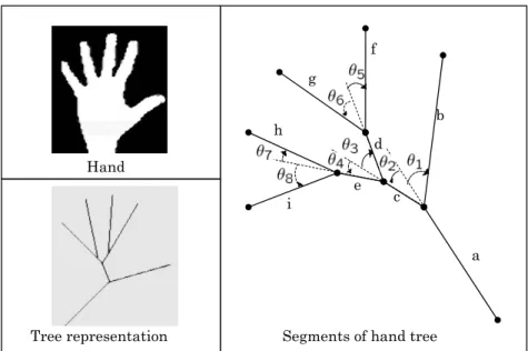
Segments of hand tree f d g c b a e h i Hand Tree representation

Figure 1.6: Hand tree representation by complex number. After preprocessing by image processing techniques the segments construct a tree, each having a length and angle.

Apart from the above examples, it is often advantageous to model two dimen-sional data as complex number field when the meaning of direction and intensity is important. For example, modeling and forecasting of wind speed and direction can be done efficiently in the complex domain. Recent studies have shown that there is a strong correlation between speed and direction of wind signal (41). Consequently, better predicting performance is achieved when wind signal is represented in complex domain, instead of taking the components independently (41). Another example is representation of hand in the hand gesture recognition system. Figure 1.6 shows a tree diagram of hand image after some signal processing. Note that each segmental element has a length and direction which can be represented by a complex number. The set

(26)

of all segments in the image constructs a complex-valued feature vector that can be fed to a pattern recognizer such as complex-valued neural network (CVNN). Excellent recognition performance by CVNN is recently reported in (19).

Since ANNs are well established efficient adaptive models it is natural and demand-ing to extend them to complex domain as we encounter information representation in complex domain. However, traditional approaches of separating complex data into valued components (real/imaginary or magnitude/phase) and then employing real-valued neural networks (RVNNs) have been proved inefficient as they do not reflect the coupling between the real-valued components (23). This has motivated to directly use complex parameters and algebra in the neural networks which is the key feature of CVNNs. Development and applications of CVNNs have seen much interest in the recent days as we can observe from several special sessions on CVNNs in the major conferences on neural networks.

It has been discovered soon after the conception of CVNN that extending ANNs to complex domain is not straight forward. The most difficulty involves in devising non-linear activation function which is the key and essential feature of nonnon-linear processing by ANNs. This limitation is a result of famous Liouville’s theorem in complex analysis: if a complex function is analytic (holomorphic) and bounded then it is a constant func-tion. As a trade-off, mostly used activation functions in the CVNNs are nonanalytic (nonholomorphic) and bounded.

Because the nonholomorphic functions do not have complex-derivative, derivation of gradient based optimization or learning algorithms require the problem to be solved in the real domain which is often tedious and hindering especially for sophisticated second order learning algorithms. Consequently, a systematic and simpler approach is needed. One possibility in this regard is to utilize theWirtinger calculus that can deal with noholomorphic complex-valued functions.

In addition to the multilayer networks in the real domain, there has been a wide deployment of single-layered structure called functional link network (FLN) for its simplicity and faster processing. Exploration and possibilities of the FLN has not yet been studied in the complex domain. In the complex domain, we may have an additional advantage of avoiding nonholomorphic activation functions when the FLN is considered as a computing model. For example, nonlinearity can be achieved in the input layer of FLN by using complex-valued polynomials.

(27)

1.2 Objectives of the thesis

Besides the processing of complex-valued data by CVNNs, there has been an in-teresting finding that a complex-valued neuron (CVN) is able to solve several well known nonlinearly separable real-valued classification problems, such as XOR,

parity-n, and symmetry detection problems. This finding suggests pattern classification as an encouraging application area of CVNNs. However, performance study of CVNNs on real-world benchmarking problems is still lacking in the literature. Therefore, a study of classification performance of simple CVNN (for example, a single CVN or single-layered CVNN) on real-world benchmark problems would be interesting.

This thesis is an effort along these aforementioned directions.

1.2 Objectives of the thesis

The following are the main objectives of the thesis:

• To utilize a convenient calculus called Wirtinger calculus for dealing with non-holomorphic functions in the complex domain, thereby simplifying the derivation of first and second order learning algorithms in the CVNNs.

• To explore complex-valued multivariate polynomial model as an alternative way of achieving nonlinearity for function approximation problems. The resulting model is known as functional link network. This polynomial approach relaxes the requirement of complex-valued activation functions and can provide faster learning.

• To perform an empirical study of using single-layered CVNNs in real-valued pat-tern classification problems and to design new activation functions for better discriminating ability.

1.3 Organization of the thesis

Chapter 2 discusses the problem of devising nonlinear activation functions in the CVNNs. First it is shown that the desirable properties of activation functions, an-alyticity and boundedness, can not be achieved in the complex domain at the same time. Then we discuss the current approaches of adopting activation functions in the literature.

(28)

Chapter 3 presents the use of Wirtinger calculus for deriving learning algorithms in the CVNNs in a simpler way. A brief introduction to the Wirtinger calculus is provided showing that it can nicely handle nonholormorphic functions while computing the derivatives. Utilization of this convenient calculus is demonstrated by deriving two most popular algorithms in the feedforward neural networks, namely, backpropagation (gradient descent) and Levenberg-Marquardt algorithm.

An alternative approach to the multilayer CVNNs termed as complex-valued func-tional link networks (CFLNs) for solving function approximation problems in the com-plex domain is presented in Chapter 4 . The CFLNs are single-layered network without hidden layer(s), where nonlinearity is incorporated in the input layer in the form of lin-early independent basis functions. Since multivariate polynomials are well defined in the complex domain just like the real domain, they are used as basis functions in the CFLNs. Furthermore, orthogonal least squares based learning algorithm is applied for designing parsimonious CFLNs that include only the relevant polynomial terms, in-stead of considering full polynomial model. The performance of CFLN is evaluated and compared on a synthetic function approximation, a nonlinear communication channel equalization and real-world wind prediction problems.

Regarding the pattern classification ability of a complex-valued neuron, an interest-ing observation is that it is more powerful than a real-valued neuron since it can solve several nonlinearly separable problems besides the linear ones, such as the XOR, the parity-n and the symmetry detection problem. This motivation is suggestive to inves-tigate how simple CVNNs like single-layered CVNNs perform on practical real-valued classification problems. In Chapter 5, we first propose two new activation functions for better discriminating ability than the existing ones. We then apply single-layered CVNNs on several real-world benchmarking problems and evaluate their performance. The performance is compared with multilayer RVNNs and shown to be comparable even though there is no hidden neuron in the CVNNs. Furthermore, in order to enhance the classification ability, ensemble approach is studied and the performance is evalu-ated over several benchmark problems with two ensemble techniques, namely, negative correlation learning (38) and bagging (8).

(29)

1.4 Major contributions

• Wirtinger calculus is utilized to derive gradient descent and Levenberg-Marquardt (LM) algorithm in multilayer feedforward CVNNs, which otherwise would have been much complicated, particularly, in deriving LM algorithm. The LM algo-rithm has much faster learning convergence and higher precision. Although LM is quite popular in the RVNNs, our contribution is the first to apply it in the CVNNs.

• Although some works on the application of FLNs in processing complex-valued data have been done, the networks are real-valued and complex-valued data is separated into real and imaginary parts thereby solving the problem in the real domain. In contrast, we consider fully complex-valued FLNs and show some advantages of considering FLNs directly in the complex domain. We have also addressed the design issue of choosing appropriate basis functions (polynomial terms) in the CFLNs.

• An empirical study on the classification and generalization ability of single-layered CVNNs has been done for several real-world benchmarking data sets with the proposal of two new activation functions. Further enhancement of classification performance is achieved by employing ensemble techniques.

(30)

(31)

Chapter 2

Activation Functions

An artificial neuron receives input signals from other neurons, and its computational procedure is to impose some weight to each input signal and to sum up the weighted input signals. We call the sum of weighted inputs as net-input of the neuron. Then the neuron yields an output signal by using a function. The function is known as activation function and generally it has nonlinear characteristic. Activation functions can also be linear, but if all the neurons in a network have linear activation function(s) the network will have a very limited processing capability.

This chapter explains various activation functions that are widely used in the neural networks. We begin with the discussion of commonly used activation functions in the real-valued neural networks(RVNNs) in Section 2.1. Section 2.2 explains the problems with the widely used activation functions when they are extended to complex domain. Section 2.3 shows how the problems are avoided at present to construct useful CVNNs.

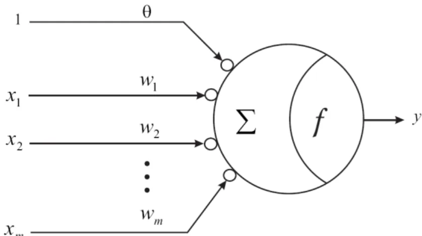
2.1 Nonlinear activation functions in real-valued neurons

Activation functions, in general, can be linear or nonlinear. We discuss only non-linear functions here because neural networks achieve their versatile processing ca-pabilities through the nonlinear characteristic of activation functions. In contrast, the networks that use only linear activation functions have a very limited processing power. Figure 2.1 shows a mathematical model of a general neuron which receives input signals xj(1≤j ≤m) and imposes a connection weight wj with each xj. This operation is the linear part of neuron yielding the net-input or internal state of the

(32)

Figure 2.1: A neuron with input signal x = (x1, x2, . . . , xm)T, connection weight w = (w1, w2, . . . , wm)T, and bias θ. The linear part combines the weighted sum

yield-ing neuron’s internal state callednet-input. The Nonlinear part transforms the net-input by an activation functionf to produce outputy.

neuron v = Pm

j=1

wjxj +θ, where θ is referred to as bias of the neuron. For a given input signal x= (x1, x2, . . . , xm)T, the neuron produces an output y with the help of activation functionf. Hence, the output is given by

y=f(v) =f   m X j=1 wjxj+θ   (2.1)

Mostly used activation functions in real-valued neurons are sigmoid functions (“S” shaped function having a saturation characteristic), such as

f(v) = 1

1 +e−v, v∈R (2.2)

The function is called log sigmoid function, and its shape is given in Fig. 2.2(a). It has a saturation characteristic at two sides. Saturation characteristic is an imitation of biological neuron. When a biological neuron receives larger input signals (higher pulse frequency), the output signal (pulse frequency) also become higher in a satura-tion manner. Besides, saturasatura-tion characteristic is important in learning algorithms for stability. Another widely used activation function is hyperbolic tangent which has the following form,

g(v) = tanh(v) = e v₋_e−v

(33)

2.1 Nonlinear activation functions in real-valued neurons −5 0 5 0 0.2 0.4 0.6 0.8 1 v f ( v ) = 1 1 + e − v (a) −5 0 5 −1 −0.5 0 0.5 1 v f ( v ) = ta n h ( v ) (b) −5 0 5 0 0.5 1 1.5 2 v f ( v ) = 1 1 + e − c v (c) −5 0 5 −2 −1.5 −1 −0.5 0 0.5 1 1.5 2 v f ( v ) = ta n h ( cv ) (d) c = 0.5 c = 1.0 c = 3.0 c = 0.5 c = 1.0 c = 3.0

Figure 2.2: Activation functions in real-valued neurons: (a) log-sigmoid, (b) hyperbolic tangent, (c) and (d) log-sigmoid and hyperbolic tangent, respectively, with amplitudeA= 2 and different gain coefficientsc={0.5,1.0,3.0}.

(34)

and its shape is shown in Fig. 2.2(b). Sometimes it is useful to introduce a gain coefficientcand/or saturation amplitude Ato control the slope and saturation values. In that case, Eqs. (2.2) and (2.3) become

f(v) = A

1 +e−cv (2.4)

g(v) =Atanh(cv) . (2.5)

Figure 2.2(c) and 2.2(d) show the effect gain coefficient and saturation amplitude. Increase in gain c yields a steeper slope, and when c _{→ ∞} the sigmoid functions approach to the step function. The gain has an effect in the learning process which may cause larger or smaller step in an iterative gradient descent algorithm. It is, however, shown that the effect of gain coefficient can be compensated by the learning rate (68).

Functions defined by Eqs. (2.2) and (2.3) are regular (no singular point(s)), bounded and differentiable in the entire domain, the set of all real numbersR. So we see here that the desirable properties of an activation function are boundedness and differentiability in the entire domain. The boundedness property is necessary for the neural networks to work as universal approximators (24). At the same time, the property of differentiability is important for many learning algorithms which are based on derivatives.

2.2 Problems with complex-valued activation functions

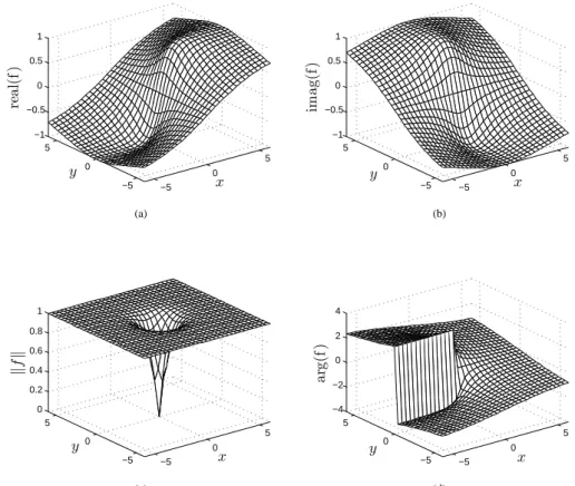
We mentioned in chapter 1 that study of CVNNs requires special considerations and that trivial extensions of RVNNs to CVNNs will not work in neural processing of complex-valued information. This section explains the reasons why such trivial exten-sion does not work.

Consider the log sigmoid-function given by Eq. (2.2). When we replacev byz_∈C, the function takes the form of f(z) = 1/(1 +e−z_{). It is easy to verify that when} _z approaches to any value in the set,

0_±j(2n+ 1)π :nis any integer andj =√₋1 ,

|f(z)_{| → ∞}. Thusf(z) is singular at regular intervals on the imaginary axis. In other words, the function is not bounded in the entire complex domain. Figure 2.3 illustrates the shape of the function, which is far away from the saturation feature seen in the real-valued case of Eq. (2.2). Similar argument follows for the function tanh(z) as

|tanh(z)_{| → ∞} whenever z approaches to any value in the setn0_±j(2n+ 1)π 2

o .

(35)

2.2 Problems with complex-valued activation functions −5 0 5 −5 0 5 −2 −1 0 1 2 3 x (a) y re a l( f) −5 0 5 −5 0 5 −5 0 5 x (b) y im a g (f ) −5 0 5 −10 0 100 1 2 3 4 5 x (c) y k f k −5 0 5 −5 0 5 −4 −2 0 2 4 x (d) y a n g le (f )

Figure 2.3: Complex-valued functionf(z) = 1/(1 +e−z_{), where}_z₌_x+_{jy. (a) real part,}

(36)

Another problem concerns with the analyticity property. Note that in the complex domain, the terms analytic and holomorphic are synonymous. A complex function is analytic in an open domain when it is differentiable at any point in that open domain. We say a complex function is differentiable, if the limit of f(z+ ∆z)−f(z)

∆z exists,

whenever ∆z → 0. Note that the limit should exist irrespective of the directions of ∆z towards zero. Another way to say the condition for complex differentiability is that a complex function is analytic in a given open domain if and only if it satisfies theCauchy-Riemann equations, everywhere in that open domain. Letz=x+jy and

f(z) =u(x, y) +jv(x, y). Then the Cauchy-Riemann equations are

     ∂u ∂x = ∂v ∂y ∂u ∂y =− ∂v ∂x

In that case, the complex derivative can be computed as

df dz = ∂u ∂x+j ∂v ∂x = ∂v ∂y−j ∂u ∂y

Due to the stringent constraints of Cauchy-Riemann equations, many real analytic functions (analytic everywhere in the real domain) do not retain analyticity property in entirety when the functions are extended to the complex domain. We already showed that sigmoid functions when extended to the complex domain have singular points. Thus, the sigmoid functions are not entire (analytic everywhere in the complex domain). If we could find some analytic function(s) that are bounded and entire we could analyze neural dynamics of CVNNs similar to the ways used in RVNNs. Such hope is, however, diminished by Liouville’s theorem which states that if a complex function is entire and bounded, then it is a constant function. Constant activation function is of no use in a neuron since the neuron will produce a constant output for all possible input signals.

It is now clear that analyticity and boundedness property poses a dilemma in CVNNs since both of the properties can not be achieved together. In fact, this has been regarded as a major concern in the development and application of CVNNs.

(37)

2.3 Construction of complex activation function with real partial derivatives

2.3 Construction of complex activation function with real

partial derivatives

One possibility for providing nonlinear activation functions in the CVNNs is to avoid singularities. That is, weight parameters and the input signals in the neurons should be selected in a way that neuron’s internal state is away from the singular points and their close neighborhoods. However, such restriction is impractical because optimization or learning procedures would be obstructed and might not converge. Moreover, we can not be sure about the values of future input signals.

Generally, the problems of activation functions in CVNNs are avoided as follows. When a nonlinear activation function is introduced, one does not pay attention to the differentiability. It does not matter whether the function is analytic or not. Importance is rather given on the boundedness property. The complex activation functions are then designed with meaningful real-valued partial derivatives of real/imaginary components. Georgiou and Kutsougeras (18), while developing complex domain backpropagation, have identified the following properties that an activation function f(z) = u(x, y) +

jv(x, y) should posses.

• f(z) is nonlinear in x and y. It is because linear activation functions will limit the capabilities of CVNNs severely.

• f(z) is bounded. This will be true only if bothu and v are bounded.

• The partial derivatives,ux,uy,vx, and vy exist and are bounded.

• f(z) is not entire. It is because if the function is entire and bounded it will be a constant function due to Liouville’s theorem.

• uxvy 6=uyvx. The reason is that the conditionuxvy =uyvx would cause a stale-mate in the adaptation of the inward connection weights of a neuron unnecessarily. See (18) for details.

A widely used activation function that follows the above properties has the following form

(38)

where fR(·) and fI(·) are generally any of the real-valued log sigmoid and hyperbolic tangent functions given by Eq. (2.2) and Eq. (2.3). This function is sometimes called

real-imaginary-type activation. Figure 2.4 shows the shape of the function with fR(·) and fI(·) being log-sigmoid function. Since the function deals with real and imagi-nary parts separately and independently, a network processingn₋dimensional complex-valued information has neural dynamics slightly similar to that of real-complex-valued neural network processing 2n−dimensional real valued information (23).

Another widely used activation function is amplitude-phase-type activation func-tion. The function is expressed as

f_C→C(z) = tanh(|z|)e

jarg(z) _(2.7)

The function deals complex numbers in polar coordinate system. It gives a saturation characteristic in the amplitude leaving the phase unchanged. Figure 2.5 shows the shape of the function. It can be seen that the function has a point symmetry around the origin (0, j0). Since waves are often represented by amplitude and phase, amplitude-phase-type activation function is suitable for processing wave-related information (23). Its saturation in amplitude can be related to the saturation of wave energy. The function is also useful to deal with time-sequential and space-sequential signals in frequency domain.

Although we presented two widely used activation functions for nonlinear mapping in a CVN, they are not limited to these two functions. Instead, we can introduce activation functions suitable for our processing purpose. For example, we propose two such functions while we discuss CVN models for classification tasks in Chapter 5.

(39)

2.3 Construction of complex activation function with real partial derivatives −5 0 5 −10 0 100 0.2 0.4 0.6 0.8 1 x (a) y re a l( f) −5 0 5 −10 0 100 0.2 0.4 0.6 0.8 1 x (b) y im a g (f ) −5 0 5 −10 0 10 0 0.5 1 1.5 x (c) y k f k −5 0 5 −10 0 10 0 0.5 1 1.5 2 x (d) y a rg (f )

Figure 2.4: Real-imaginary-type complex activation function: (a) real part, (b) imaginary part, (c) amplitude, and (d) phase of the function.

(40)

−5 0 5 −5 0 5 −1 −0.5 0 0.5 1 x (a) y re a l( f) −5 0 5 −5 0 5 −1 −0.5 0 0.5 1 x (b) y im a g (f ) −5 0 5 −5 0 5 −4 −2 0 2 4 x (d) y a rg (f ) −5 0 5 −5 0 5 0 0.2 0.4 0.6 0.8 1 x (c) y k f k

Figure 2.5: Amplitude-phase-type complex activation function: (a) real part, (b) imagi-nary part, (c) amplitude, and (d) phase of the function.

(41)

Chapter 3

Wirtinger Calculus based

Learning Algorithms

3.1 Introduction

The key features of complex-valued neural networks (CVNNs) is that their parameters are complex numbers and they use complex algebraic computations. However, the most important matter is to devise learning algorithms for them. Gradient or derivative based algorithms are perhaps the most prevalent learning mechanisms in the neural networks. As we have seen in Chapter 2, unlike real-valued neural networks (RVNNs) the standard complex derivative for the widely used complex-valued activation functions does not exist because they arenonholomorphic functions.

In fact, the CVNNs bring in nonholomorphic functions in two ways: (i) with the loss function to be minimized over the complex parameters and (ii) the most widely used activation functions. The former is completely unavoidable as the loss function is necessarily real-valued. The second source of nonholomorphism arises because bound-edness and analiticity cannot be achieved at the same time in the complex domain, and it is the boundedness that is often preferred over analyticity for the activation functions (49). Although some researchers have proposed some holomorphic activation functions having singularities (31), a general consideration is that the activation functions can be nonholomorphic. In such a scenario, optimization algorithms are unable to use standard complex derivatives, since the derivatives do not exist (i.e., theCauchy-Riemann equa-tions do not hold). As an alternative, conventional approach for algorithm derivation

(42)

cast the optimization problem in the real domain and use the real derivatives, which often requires a tedious computational labor. Here computational labor is meant for human efforts associated with the calculation of derivatives in analytic form.

An elegant approach that can save computational labor in dealing with nonholomor-phic functions is to use Wirtinger calculus (71). The Wirtinger calculus can be con-sidered as a generalization of complex derivative using conjugate coordinates, where two derivatives ∂f_∂z and _∂z∂f∗ come in a pair. The derivatives are called R-derivative and conjugate R-derivative, respectively. The formal definitions and properties of the derivatives are discussed in Section 3.2.

A pioneering work that utilizes the concept of conjugate coordinates is by Brand-wood (7). The paper formally defines complex gradient and the condition for stationary point. It also discusses an application in adaptive array theory. The work is further ex-tended by van den Bos showing that complex gradient and Hessian are related to their real counterparts by a simple linear transformation (70). However, neither of the au-thors has cited the contribution of Wilhelm Wirtinger, a German mathematician, who originally developed the concept of derivatives with respect to conjugate coordinates. The reason might be due to the fact that the article was published in the German lan-guage. Today, Wirtinger calculus is well-appreciated and has been fruitfully exploited by several recent works (6, 36).

Although Wirtinger calculus can be a useful tool in adapting well known first- and second-order optimization algorithms used in the RVNN to the CVNN framework, only few studies can be found in the literature (35). In (35), Wirtinger calculus has been utilized to derive a gradient descent algorithm for a feedforward CVNN. The authors employ holomorphic activation functions and states that the derivation is simplified only because of the holomorphic functions. It is further stated that the evaluation of gradient in nonholomorphic case has to be performed in the real domain as it is done traditionally.

In Section 3.3, we show that Wirtinger calculus can simplify the gradient evalu-ation in nonholomorphic activevalu-ation functions too, which is the original motivevalu-ation of Wirtinger calculus. Our gradient evaluation is more general and CVNN with holomor-phic activation function becomes a special case only.

Besides the gradient descent algorithm, we derive a popular second-order learning method (in the sense, the Hessain matrix involving second order derivatives is

(43)

ap-3.2 Wirtinger calculus

proximated by using Jacobian matrix), Levenberg-Marquardt (LM) algorithm (21), for CVNN parameter optimization. The derivation is provided in Section 3.4. We find that a key step of LM algorithm is a solution to the least squares problem_kb₋(Az+Bz∗)_kmin

z

in the complex domain, which is more general than the_kb₋Az_kmin

z . Here z

∗ _denotes

the conjugate of a column vector z. A solution to the least square problem has been given with a proof. All computations regarding gradient descent and LM algorithm are carried out in matrix-vector form that can be easily implemented in any computational environment where computations are optimized for matrix operations.

An important aspect of our derivations is that we use functional dependency graph for a visual evaluation method of derivatives, which is particularly useful in multilayer CVNNs. Because Wirtinger calculus essentially employs conjugate coordinates, a coor-dinate transformation matrix between the real and conjugate coorcoor-dinates system plays an important role in adapting derivative based algorithms in the RVNNs to the CVNNs. It turns out that the Wirtinger calculus, the coordinate transformation matrix, and the functional dependency graph are three useful tools for adapting optimization algorithms in RVNNs to the CVNN framework.

Computer simulation results are presented in Section 3.5 in order to validate the derived algorithms. The results exhibit that as with real-valued case, the complex-LM algorithm provides much faster learning than the complex-gradient descent algorithm. Although the LM algorithm is widely used in the RVNN training, no other study except ours (3) has been done in the complex domain. We summarize the key concepts of this chapter in Section 3.6,.

3.2 Wirtinger calculus

This section briefly discusses theR-derivative and the conjugateR-derivative formally developed by a German mathematician, Wilhelm Wirtinger (71). The resulting calculus is therefore also known as Wirtinger calculus in the literature. Rigorous descriptions with applications can be found in (7, 32, 46, 60).

Any function of a complex variable z can be defined as f(z) = u(x, y) +jv(x, y),

where z = x+jy. If all the partial derivatives ux, uy, vx, and vy exist, then the complex derivative off(z) is said to exist if the partial derivatives satisfy the Cauchy-Riemann equations, i.e., ux = vy, vx = −uy. In the complex domain, the functions

(44)

satisfying the Cauchy-Riemann equations are called holomorphic functions. Otherwise, the functions are called noholomorphic. As for instance, if a functionf(z) is real-valued, i.e., v(x, y) = 0, then it is nonholomorphic since the Cauchy-Riemann equations no longer hold. Thus the Cauchy-Riemann equations are more stringent condition then the mere existence of partial derivatives. Consequently, we do not have a definition of complex derivate for nonholomorphic functions.

Interestingly, any differentiable mapping, f : R2 → R2(orR), can be treated in complex domain by introducing conjugate coordinates such that

z z∗ = 1 j 1 −j x y . (3.1)

This ingenious idea of Wirtinger allows us to deal with nonholomorphic functions in the complex domain. In other words, any nonholomorphic mapping f :C→ C(orR) is viewed from real perspective, but in terms of conjugate coordinates. Note from Eq. (3.1) that the conjugate coordinates are related to the real coordinates by a simple coordinate transformation matrix. From the inverse relations, x = (z +z∗₎_/_{2 and}

y = ₋j(z₋z∗)/2, Wirtinger defines the following pair of derivatives for a function

f(z, z∗_): ∂f ∂z = 1 2 ∂f ∂x−j ∂f ∂y , ∂f ∂z∗ = 1 2 ∂f ∂x+j ∂f ∂y . (3.2)

The derivatives are called R-derivative and conjugateR-derivative, respectively. From the coordinate transformation view point, one can take partial derivatives in either of the coordinate systems, whichever seems convenient. Then, if required, it is straightforward to switch to the other coordinate system by the simple linear transfor-mation. When evaluating partial derivatives in the conjugate coordinate system, we take one of the variables,z and z∗_{, as constant. For example, in the evaluation of} ∂f

∂z,

z∗ is considered as constant; similarly in the evaluation of _∂z∂f∗,zis taken as a constant. An illustrative example is given belew.

Example Supposeg(z, z∗) =z2_z∗₌_u₊_jv_{, where}_z₌_x₊_jy_{, then}

u(x, y) =x3₊_xy2

(45)

3.2 Wirtinger calculus ∂g ∂z = 1 2 ∂ ∂x−j ∂ ∂y (u+jv) = 1 2 3x 2₊_y2₊_j₍₂_xy₎ −j 2xy+j(x2+ 3y2) = 2(x2+y2) = 2zz∗ ∂g ∂z∗ = 1 2 ∂ ∂x+j ∂ ∂y (u+jv) = 1 2 3x 2₊_y2₊_j₍₂_xy₎ +j 2xy+j(x2_{+ 3}_y2₎ =x2₋y2+j2xy =z2

Here the derivatives are computed in the real coordinate system defined in Eq. (3.2). However, one can get the similar results quickly if the derivatives are evaluated in the conjugate coordinate system. That is, ∂(z

2_z∗₎

∂z = 2zz

∗ _and ∂(z2_z∗₎

∂z∗ =z2.

Most importantly, Wirtinger calculus generalizes the concept of derivatives in com-plex domain. It is easy to see that the Cauchy-Riemann equations are equivalent to

∂f

∂z∗ = 0. In other words, the holomorphic functions are functions of z only, not z∗. This beautiful result is the key to deal with nonholomorpic functions in the gradient based optimization problems involving complex-valued parameters. There is no need to express the optimization problem in the real domain which would be tedious and cumbersome. Readers can check our derivations presented in Section 3.3 with the other real domain derivations found in the literature, e.g., (18, 34, 62).

Wirtinger calculus enables us to perform all computations directly in the complex domain, and the derivatives obey all the rules of conventional calculus, including the chain rule, differentiation of products and quotients. Here are some useful identities that we use extensively in the derivation of learning algorithms of Section 3.3 and Section 3.4. ∂f ∂z ∗ = ∂f ∗ ∂z∗; when f is real ∂f ∂z ∗ = ∂f ∂z∗ [Conjugation rule] (3.3) ∂f ∂z∗ ∗ = ∂f ∗ ∂z ; whenf is real ∂f ∂z∗ ∗ = ∂f ∂z [Conjugation rule] (3.4)

(46)

df = ∂f ∂zdz+ ∂f ∂z∗dz ∗ [Differential rule] (3.5) ∂h(g) ∂z = ∂h ∂g ∂g ∂z + ∂h ∂g∗ ∂g∗ ∂z [Chain rule] (3.6) ∂h(g) ∂z∗ = ∂h ∂g ∂g ∂z∗ + ∂h ∂g∗ ∂g∗ ∂z∗ [Chain rule] (3.7)

3.3 Gradient descent algorithm

The gradient of a real-valued scalar function of several complex variables can be eval-uated in both real and conjugate coordinate systems. And there is a one to one corre-spondence between the coordinate systems. Let zbe an n-dimensional column vector, i.e., z= (z1, z2, . . . , zn)T ∈Cn, wherezi =xi+jyi,i= 1,2, . . . , n. Then

c, z z∗ ⇔r, x y = <(z) =(z) ,

where _<(z) and ₌(z) represent the real and imaginary parts of z, respectively. In the real-valued coordinates, the gradient is defined as

real-∇f = ∂f ∂x1 , ∂f ∂x2 , . . . , ∂f ∂xn , ∂f ∂y1 , ∂f ∂y2 , . . . , ∂f ∂yn T = ∂f xT, ∂f yT T , (3.8)

whereT denotes the ordinary transpose operator. Now if the real-valued partial deriva-tives are arranged according to the real and imaginary parts, component-wise, an in-tuitive definition of complex gradient could be

complex-_∇f = ∂f ∂x1 +j∂f ∂y1 , . . . , ∂f ∂xn +j∂f ∂yn T = 2∂f ∂z∗ 1 , . . . ,2∂f ∂z∗ n T = 2∂f ∂z∗ ,∇z∗f , (3.9)

The second line of Eq. (3.9) follows from Eq. (3.2). As will be shown next, a more formal derivation leads to the same definition of Eq. (3.9).

(47)

3.3 Gradient descent algorithm

In the single complex variable case, real and conjugate coordinates are related by the coordinate transformation matrix of Eq. (3.1). Similarly, the multivariable case can be written with a coordinate transformation matrix in the block matrix form

c= z z∗ = I jI I ₋jI x y =J x y =Jr , (3.10)

where I is an identity matrix conforming to the size of x or y. Note here that

J−1 = 1₂JH, where H represents Hermitian transpose operation. Since the coordi-nate transformation is a linear transformation it follows that for a real-valued scalar function,f(z,z∗), ∂f ∂r = ∂cT ∂r ∂f ∂c =J T∂f ∂c .

Since bothf and rare real-valued ∂f ∂r = ∂f ∂r ∗ = JT∂f ∂c ∗ =JH ∂f ∂c∗ . [Equation (3.3)]

The gradient descent update rule in the real-valued case is ∆r=−µ∂f

∂r, where µis a

small step size. Using the coordinate transformation of Eq. (3.10), we obtain

∆c=J∆r=₋µJ∂f ∂r =−µJJ H ∂f ∂c∗ =−2µ ∂f ∂c∗ . (3.11)

Becausec∗= (z∗,z)T, Eq. (3.11) can be written as

∆c= ∆z ∆z∗ =−2µ      ∂f ∂z∗ ∂f ∂z      ⇒∆z=−2µ∂f ∂z∗ . (3.12)

Thus using the Wirtinger calculus, the complex-gradient of a real-valued function with respect to a parameter vector z is evaluated as _∇z∗f = 2∂f

∂z∗, but not

∂f

∂z! Note

that this formal way of formulation conforms to our intuitive definition of Eq. (3.9). Although the multiplicative factor 2 appearing in the complex-gradient may be ignored, we adhere to this as the exact relationship between the real-gradient (had we solved the optimization problem in the real domain) and the complex-gradient should include

(48)

the factor. Thereby, one can verify the final result of derivation in the real domain with that in the complex domain and appreciate the simplicity obtained in complex domain due to the Wirtinger calculus. No matter, whichever approach is followed the final result must be same, but the Wirtinger calculus is much more elegant and painless.

Now that we have the notion of complex-gradient, we are ready to derive the gradi-ent descgradi-ent learning algorithm in feedforward CVNN. We will consider a single hidden layer CVNN for the sake of notational convenience only. The method presented here, however, can be easily followed for any number of layers. The derivation is carried out in matrix-vector form. As a result, the algorithm can be easily implemented in any computing envirionment, where matrix computations are optimized.

The forward equations for signal passing through the network are as follows

y=Vx+a [linear transform part: input_→ hidden] (3.13a)

h=φ(y) [nonlinear transform in the hidden layer] (3.13b)

v=Wh+b [linear transform part: hidden_→ output] (3.13c)

g=φ(v) [nonlinear transform in the output layer] , (3.13d)

where x is the input signal and h and g are the outputs at hidden and output layer, respectively; the weight matrix V connects the input units to the hidden units, while the matrixW connects the hidden units to the output units; the column vectorsaand

b are the biases to the hidden and output units, repectively; andφ(·) is any activation function (holomorphic or nonholomorphic) having real partial derivatives. When the argument to the function is a column vector it operates element wise, resulting another column vector with the same dimension. Note that all the vectors and matrices in Eq. (3.13) are complex-valued.

Supervised learning algorithm provides the network a desired signal d, from which an error signal can be computed as

e=d₋g (3.14)

Then the gradient descent algorithm minimizes a real-valued loss function

ξ(z,z∗) = 1 2 X k e∗_kek= 1 2e H_e _, _(3.15)

(49)

which depends on parameter vectorzas well as its conjugatez∗. The parameter vector

zis iteratively updated along the opposite direction of gradient, i.e., to the negative of gradient. The negative of complex gradient as defined in Eq. (3.12) can be written as

−∇z∗ξ=−2 ∂ξ ∂z∗ =−2 ∂ξ ∂z ∗ =₋2 ∂ξ ∂zT H [Eq. (3.3)] . (3.16)

We find that it is convenient to take derivative of a scalar or a column vector with respect to a row vector as it gives the Jacobian naturally. Now

−2 ∂ξ ∂zT =− ∂ eHe ∂eT ∂e ∂zT − ∂ eHe ∂(eT₎∗ ∂e∗

∂zT [Eq. (3.6) in matrix-vector form] =eHJz+eT(Jz∗)∗ . [Eq. (3.4) in matrix-vector form] (3.17)

Here, we define two Jacobian matrices,Jz=

∂g

∂zT andJz∗=

∂g

∂(z∗₎T. Taking Hermitian conjugate transpose to both side of Eq. (3.17) yields the negative of complex-gradient as

−∇z∗ξ =JH

ze+ JHz∗e ∗

. (3.18)

It is clear from Eq. (3.18) that in order to evaluate complex-gradient all we need to compute is a pair of Jacobians: Jz, the Jacobian of network output g w.r.t. the parameter vector z; and Jz∗, the Jacobian of g w.r.t. z∗. It should be noted that the Jacobians have the form ofP+jQand P−jQ, respectively, because of the definition of derivatives in Wirtinger calculus. Consequently, we can compute the other one while computing one of the Jacobians.

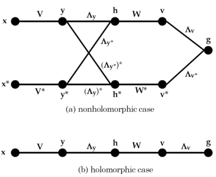
Visual evaluation of Jacobians in CVNN:In the feedforward CVNN, parameters

are structured in layers. We find that it is very much efficient to compute the Jacobians visually if we draw a functional dependency graph, where each node denotes a vector-valued functional and each edge connecting two nodes is labeled with the Jacobian of one node w.r.t. the other node. Figure 3.1 depicts the functional dependency graph for a single hidden layer CVNN. Each edge is labeled with the Jacobian of its right node w.r.t. its left node. However, the Jacobians of interest are Jz and Jz∗, i.e., the Jacobians of the rightmost node (labeled asgin Fig. 3.1) with respect to all the nodes appearing to its left at different depths.

To evaluate the Jacobian of the right most node (i.e., network’s output) w.r.t. any other node to its left, we just need to follow the possible paths from the right most

(50)

Figure 3.1: Functional dependency graph of a single hidden layer CVNN corresponding to Eq. (3.13). Each node represents a complex-vector-valued variable, and an edge connecting two nodes is labeled with the Jacobian of its right node with respect to its left node. (a) The general case, activation functions are nonholomorphic and (b) the special case, activation functions are holomorphic. In the holomorphic case, conjugate Jacobians are the zero matrix. Thus, graph (a) reduces to graph (b).

(51)

node to that node. Then the desired Jacobian is the sum of all possible paths, where for each path the labeled Jacobians are multiplied from right to left. For example in Fig. 3.1,

Jy=

∂g

∂yT

= ΛvWΛy+ Λv∗W∗(Λ_y∗)∗ , (3.19)

where the Jacobians Λv, Λy, Λv∗, and Λy∗are diagonal matrices and computed from the activation functions according to Eq. (3.2). As an example, let v = (v1, v2, . . . , vm)T. Then Λv=       ∂φ(v1) ∂v1 0 . . . 0 0 ∂φ_∂v(v2) 2 . . . 0 .. . ... . .. ... 0 0 . . . ∂φ_∂v(vm) m       Λv∗ =        ∂φ(v₁∗) ∂v∗ 1 0 . . . 0 0 ∂φ(v∗2) ∂v∗2 . . . 0 .. . ... . .. ... 0 0 . . . ∂φ(vm∗) ∂v∗ m       

It may seem that the number of paths would increase in multiplicative manner for many layers network, particularly when evaluating the Jacobian at a far node than the right most node. Here a trick is to reuse the computation. We only need to look for Jacobian to the immediate rightmost nodes, presumably the Jacobian are already computed there. Thus Eq. (3.19) can be alternatively computed as

Jy=JhΛy+Jh∗(Λy∗)∗ , whereJh= ∂g ∂hT andJh∗ = ∂g ∂(h∗)T.

It is now a simple task to find the update rule for the CVNN parameters. We note from Eq. (3.13) thatJb=Jv andJa=Jy. Thus update rules for the biases at hidden and output layer are

∆a=µJH_ae+ JH_a∗e ∗

; ∆b=µJH_be+ JH_b∗e ∗

, (3.20)

where µ is the learning rate. Extending the notation for vector gradient to matrix gradient of a real-valued scalar function (35) and using Eq. (3.13), the update rules for hidden and output layer weight matrices are given by

(52)

This completes the derivation of the gradient descent learning algorithm in the CVNN. All computations are directly performed in the complex domain in matrix-vector form. As shown in Fig. 3.1 one can easily compute the required Jacobians visually from the functional dependency graph. Furthermore, if the activation function is holomorphic, the Jacobians corresponding to conjugate vector turns into zero. Consequently, Fig. 3.1(a) reduces to Fig. 3.1(b).

3.4 The Levenberg-Marquardt algorithm

The naive gradient descent method presented above has a limitation in many practical applications of multilayer neural networks because of very long training time and less accuracy in the network mapping function (4). In order to overcome this problem, many algorithms have been applied in the neural networks, such as conjugate gradient, New-ton’s method, quasi-Newton method, Gauss-Newton method, andLevenberg-Marquardt

(LM) algorithm. Among those, perhaps the LM algorithm is the most popular in the neural networks as it is computationally more efficient. In this section, we derive the LM algorithm for training feedforward CVNNs. The LM is basically a batch-mode fast learning algorithm with a modification to the Gauss-Newton algorithm. Therefore, the Gauss-Newton algorithm will be first derived in the complex-domain.

The Gauss-Newton method iterativelyre-linearizes the nonlinear model and update the current parameter set according to a least squares solution to the linearized model. In the CVNN, the linearized model of network output g(z,z∗) around (ˆz,zˆ∗) is given by g(ˆz+ ∆z,ˆz∗+ ∆z∗)_≈g(ˆz,ˆz∗) + ∂g ∂zT ˆ z∆z + ∂g ∂(z∗₎T ˆ z∗∆z ∗ = ˆg + Jz∆z + Jz∗∆z∗ . (3.22)

The error associated with the linearized model is given by

e= ˆe₋(Jz∆z+Jz∗∆z∗) , (3.23)

where ˆe = d₋ˆg is error at the point (ˆz,ˆz∗). Then the Gauss-Newton update rule is given by the least squares solution to _kˆe₋(Jz∆z+Jz∗∆z∗)k. So we encounter a more general least squares problem having the form of_kb₋(Az+Bz∗)_kmin

z , than the

well known problem,_kb₋Az_kmin