https://doi.org/10.5194/gmd-13-4435-2020 © Author(s) 2020. This work is distributed under the Creative Commons Attribution 4.0 License.
A mass- and energy-conserving framework for using machine
learning to speed computations: a photochemistry example
Patrick Obin Sturm1,3and Anthony S. Wexler1,21Air Quality Research Center, University of California, Davis, CA 95616, USA
2Departments of Mechanical and Aerospace Engineering, Civil and Environmental Engineering, and Land, Air and Water
Resources, University of California, Davis, CA 95616, USA
3Institute of Mathematics, Technical University of Berlin, 10587 Berlin, Germany
Correspondence:Patrick Obin Sturm ([email protected]) Received: 31 March 2020 – Discussion started: 28 April 2020
Revised: 10 July 2020 – Accepted: 31 July 2020 – Published: 22 September 2020
Abstract.Large air quality models and large climate models simulate the physical and chemical properties of the ocean, land surface, and/or atmosphere to predict atmospheric com-position, energy balance and the future of our planet. All of these models employ some form of operator splitting, also called the method of fractional steps, in their structure, which enables each physical or chemical process to be simulated in a separate operator or module within the overall model. In this structure, each of the modules calculates property changes for a fixed period of time; that is, property values are passed into the module, which calculates how they change for a period of time and then returns the new property val-ues, all in round-robin between the various modules of the model. Some of these modules require the vast majority of the computer resources consumed by the entire model, so increasing their computational efficiency can either improve the model’s computational performance, enable more realis-tic physical or chemical representations in the module, or a combination of these two. Recent efforts have attempted to replace these modules with ones that use machine learning tools to memorize the input–output relationships of the most time-consuming modules. One shortcoming of some of the original modules and their machine-learned replacements is lack of adherence to conservation principles that are essential to model performance. In this work, we derive a mathemat-ical framework for machine-learned replacements that con-serves properties – say mass, atoms, or energy – to machine precision. This framework can be used to develop machine-learned operator replacements in environmental models.
1 Introduction
Complex systems require large models that simulate the wide range of physical and chemical properties that govern their performance. In the air quality realm, models include CMAQ (Foley et al., 2010), CAMx (Yarwood et al., 2007), WRF-Chem (Grell et al., 2005), and GEOS-WRF-Chem (Eastham et al., 2014). In the climate change arena, models include HadCM3 (Jones et al., 2005), GFDL CM2 (Delworth et al., 2012), ARPEGE-Climat (Somot et al., 2008), CESM (Kay et al., 2015), and E3SM (Golaz et al., 2019). These models employ operator splitting, also called the method of fractional steps (Janenko, 1971), in their structure so that each module can be tasked with representing one or a small number of physical and/or chemical processes. This modular structure enhances model maintenance and sustainability while enabling diverse physical and chemical processes to interact. Each module is tasked with simulating its processes over a fixed period of time, each module called in turn until they have all re-turned their results. Usually, the computational performance of these models is governed by one or two modules that con-sume the vast majority of the computer resources. In air qual-ity models, this is usually the photochemistry and/or aerosol dynamics modules. In climate models, this is usually the ra-diative energy transport module.
Machine learning has been used to improve the compu-tational efficiency of modules in atmospheric models for decades (Potukuchi and Wexler, 1997). As machine learn-ing algorithms have improved, these efforts have matured (Hsieh, 2009; Kelp et al., 2018; Rasp et al., 2018; Keller and
Evans, 2019; Pal et al., 2019). But the effort to replace phys-ical and chemphys-ical operators with machine-learned modules is challenging because small systematic errors can build. For instance, a 0.1 % error over a 1 h time step could lead to a 72 % error after a month of simulation. This problem is com-pounded if the replacement module does not conserve quan-tities that are essential to model accuracy, such as atoms in a photochemical module, molecules and mass in an aerosol dynamics module, or energy in a radiative transfer module.
Recent efforts at developing and using machine-learned replacement modules has focused on memorizing how the quantities change. Some have also explored enforcing phys-ical constraints when memorizing these quantities via post-prediction balancing approaches (Krasnopolsky et al., 2010), introducing a penalty into the cost function (Beucler et al., 2019) or incorporating hard constraints on a subset of the output in neural network architecture (Beucler et al., 2019). All of these approaches focus on memorizing how quanti-ties change and incorporate some correction strategy after all or a portion of the quantities have been predicted. If instead we focus on how the fluxes between quantities change, we can guarantee adherence to conservation principles to ma-chine precision without a postprediction correction. In pho-tochemical modules, the fluxes are how atoms move between chemical species as reactions progress. In aerosol dynamics, the fluxes are the condensation and evaporation or coagula-tion processes that move material between the gas and parti-cle phases or between partiparti-cle sizes. In radiative transfer, the fluxes are the energy movements between spatial domains.
In this work, we derive a mathematical framework that en-ables the use of machine learning tools to memorize these fluxes. We focus this work on atmospheric photochemistry and provide an example for a simple photochemical reaction mechanism because the number of species and the complex-ity of the problem exercises many aspects of the framework.
2 Derivation of the framework for photochemistry In general, the atmospheric chemistry operator solves
∂C
∂t =F(C, T ,RH,actinic flux, stability,etc.) , (1)
whereCis a vector containing the current concentration of the chemical species,T is temperature, and RH is the relative humidity. A full list of symbols can be found in Appendix A. The right-hand side can be written as
F =AR, (2)
whereAis a matrix describing the stoichiometry, andRis a vector of reactions. The form of the right-hand side assures mass balance because it is composed of reactions that de-stroy one species while creating one or more other ones, all in balance, described by A. The R terms take forms such
as kCiCj, where k is the rate constant for a reaction
be-tween species;J Ci, whereJ is the photolysis reaction rate;
ork(Ci(x1)−Ci(x2)), wherekis a diffusion or mass
trans-port rate constant between two spatial locations or between the gas and particle phases.
In the method of fractional steps, all modules integrate their equations forward for a fixed time step,1t, that we call the operator-splitting time step. Combining these two equa-tions and integrating gives
1Ci= X j Ai,j t+1t Z t Rj(t )dt= X j Ai,jSj, (3a) or in matrix form 1C=AS, (3b) whereSj equalsRt +1t
t Rj(t )dt.Sj is the flux integral. For
atmospheric photochemistry, it is the flux of atoms between molecules. For aerosol dynamics, it is the flux of molecules condensing on or evaporating from particles or the flux of small particles coagulating on large particles. For radiative transfer,Sjis the energy between spatial coordinates. We are
able to pull theAout of the integral if it is a constant, which is usually the case or can be approximated as such.
Using machine learning tools to learn the relationship
S=S(C, T ,RH,actinic flux,stability,etc.) (4)
has advantages over memorizing a concentration– concentration relationship because of the following:
a. The formulation in Eq. (3) conserves mass.
b. TheR terms are simpler to memorize because they do not contain the complexity inA.
c. There are fewer concentrations directly influencing S
thanC, so the machine learning algorithm should be simpler.
The difficulty resides in developing the training and test-ing sets needed to train and test the machine learntest-ing algo-rithm corresponding to Eq. (4). In principle, we can run a model many times, generate a data set, and then learn that data using machine learning techniques. That is, we can run many models that integrate Eq. (1) to find the relationship between concentrations at two time steps to develop our ma-chine learning training set. But such models do not provide the value ofS, and since the chemical system is stiff, the inte-grators make many complex calls to calculate the right-hand side of Eq. (1) and integrate it. Another way of saying this is that the1Cis easily available from the models, but theSis not.
If we have many sets of1Cvalues, in principle we can invert Eq. (3b) to obtain the correspondingSvalues. The dif-ficulty with this approach is that there are more elements of
Sthan1C, so a conventional inverse cannot be applied. In-stead, we employ the generalized inverse ofAto obtainSvia the relationship
S=AG1C, (5)
whereAG is the generalized inverse ofA. In the case that there are as many fluxes as quantities (A is a square ma-trix), and the quantities are coupled but linearly dependent (Ais full rank), thenAG is the true inverse ofAand read-ily calculable. If the system is overdetermined, whereAis a rectangular matrix with more quantities than fluxes but has full column rank, then a left inverse can calculate AG. An
overdetermined system is typical in an aerosol module cal-culating condensation and evaporation, where fluxes depend on two quantities. However, ifAis underdetermined, mean-ing there are more fluxes than known quantities, orAis oth-erwise rank-deficient from linear dependency, there is an in-finite number of generalized inverses AG. This means that given values for1C, Eq. (5) will not give reliable values for
S.
Given sufficient constraints, AG will be unique and pro-vide the desired values ofSthat are needed to develop a ma-chine learning training set. Ben-Israel and Greville (2003) show that the inverse can be unique if the solutions, S, are restricted to lie in a subspace that defines the “legal” solu-tions, and these restrictions are sufficiently constraining. The constrained generalized inverse ofAproduces solutions,S, that lie in the legal subspace defined by good examples of solutions.Sis given by
AGS =PS(APS)G, (6)
where AGS is the generalized inverse of Arestricted to the subspace of all possible solutions by the projectionPS, which
in turn is defined by a set of basis vectors that define the subspace. Before we discuss obtaining the basis vectors, we first need to discuss how to obtain the projection,PS.
Assume for the moment that we have the basis vectorsSk.
We concatenate them (column-wise) to form the matrixU:
U= hS1|S2|. . .|Ski. (7)
The projection onto the subspace defined by these basis vec-torsSkand the matrixUis then (Mukhopadhyay, 2014)
PS=U U+U
−1
U+, (8)
whereU+is the transpose ofU.
Atmospheric-chemistry problems are stiff, so the U+U may be ill-conditioned. One source of this ill-conditioning, which can also hamper machine learning tools, is that the concentrations are often orders of magnitude apart. The mod-ules use actual concentrations to make the mechanism eas-ier to understand and debug. Normalizing the concentrations helps with both learning and stiffness and ill-conditioning.
Ill-conditioned problems can hamper matrix inversion. Since theSvectors describe the subspace where the solutions must reside, their magnitude does not matter, just their direction. So we normalize theSvectors by dividing by the average of the nonzero values. Mathematically, we form a diagonal square matrix,NS, with the averages on the diagonal and
cal-culate the normalizedSwith
Snorm=N−S1S. (9)
SinceNS is diagonal, the inverse is simply the reciprocal of
each diagonal element. The1C values are recovered from theSnormvalues via
1C=ANSSnorm. (10)
Atmospheric-chemistry problems are also high-dimensional. Typical air quality models may have 100 to 200 chemical species, and since the vertical-column-mixing timescale is similar to the slower timescales of the chemistry, some mod-els solve the vertical transport and chemistry simultaneously. Since typical air quality models have 10 to 20 vertical cells, the dimension of the problem is 1000 to 4000. Even though the inverse(U+U)−1only has to be calculated once, this in-version may be intractable. Providing that the condition num-ber ofU+Uis not too large, Gram–Schmidt orthonormaliza-tion can be performed on theSi vectors before carrying out
Eqs. (7) and (8), in which case they will describe the same subspace, but now the matrixU+Uwill be the identity
ma-trix, which is its own inverse.
Now let us return to the question of how to find the basis vectors that define the “legal” subspace ofS. These can be developed by solving Eq. (1) using Euler’s method, in which case Eq. (3) becomes
1Ci∼Ai,kRk(t )1t∼Ai,kSk, (11)
that is
Sk∼Rk(t ) 1t. (12)
The value of 1t does not matter since it just changes the length ofSk, not its direction and therefore not its value in
describing the subspace. The original module that calculates
Rk can be run many times under many conditions to
gener-ate a set ofSkvectors that span the subspace. Then
locality-preserving projections (LPPs), principal component analysis (PCA), or another similar algorithm can be used to find a minimum set of vectors that define the subspace.
3 Solution procedure for a photochemical module The following overview aims to put into context the pro-cedure outlined in this paper. The focus of this paper is on deriving and conducting the mass balancing framework and inverse problem detailed in steps 1–9. Steps 10–13 are pro-vided for context: these include machine learning, operator
replacement, and benchmarking. In principle, any machine learning algorithm can be used with the framework described here in steps 1–9.
1. Determine which species are active in the photochem-ical mechanism, that is, not the steady-state or buildup species.
2. From the mechanism, extract the A matrix for these species.
3. Using a representative set of atmospheric concentra-tions,T, RH, and actinic flux, use Eq. (10) and the pho-tochemical module to generate data that match values of1CandSfor many values ofC,T, RH, and actinic flux for the models operator-splitting time step. 4. Normalize theSvectors by dividing each by the average
of its nonzero elements. Use these averages to form the NSmatrix, which relatesStoSnormvia Eq. (9).
5. Use theSnormvectors and Eq. (7) to form theUmatrix
and then theU+Umatrix. What is the condition number of theU+Umatrix? If the system is large and not ill-conditioned, use Gram–Schmidt orthonormalization on theSvectors before calculatingUandU+U, in which caseU+Ushould be an identity matrix or a subset of one.
6. Use Eq. (8) to calculatePS.
7. Use Eq. (6) to calculate the constrained generalized in-verseAGS.
8. Use Eq. (5) to calculate values ofSfrom the values of
1C.
9. Compare the values ofSobtained from steps 3 and 7 to make sure they are very similar, using the dot product to calculate the angle between them. If they are, we have a goodAGS.
10. Use neural networks or another machine learning algo-rithm to memorize theS(C)relationship obtained using (a) Eq. (5) and (b) many runs of the mechanism for a wide range ofC,T, RH, and actinic flux values. 11. Replace the mechanism with the neural network to
cal-culateS(C)and Eq. (3b) to march forward. 12. Clock the speed improvement.
13. Calculate standard measures of performance such as mass balance, bias, and error compared to runs using the complete mechanism.
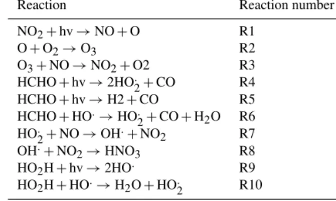
Table 1.Reaction mechanism.
Reaction Reaction number NO2+hv→NO+O R1 O+O2→O3 R2 O3+NO→NO2+O2 R3 HCHO+hv→2HO.2+CO R4 HCHO+hv→H2+CO R5 HCHO+HO.→HO.2+CO+H2O R6 HO.2+NO→OH.+NO2 R7 OH.+NO2→HNO3 R8 HO2H+hv→2HO. R9 HO2H+HO.→H2O+HO.2 R10
Table 2.Active species.
O3 NO NO2 HCHO HO.2 HO2H 4 Photochemical mechanism
We tested the methods described above on the follow-ing very simplified set of photochemical reactions used by Michael Kleeman at the University of California, Davis, when teaching the modeling of atmospheric photochemistry. Although this mechanism is abbreviated, it contains the es-sential components of all atmospheric photochemical mech-anisms related to ozone formation: NOx chemistry, volatile
organic compound (VOC) chemistry, and the formation of peroxy radicals from VOC chemistry that then react with NO to form NO2and OH, both of which may react to terminate.
The 10 reactions are given in Table 1. The oxygen atom and hydroxyl radical are assumed to be in a steady state, so there are six active species, which are listed in Table 2.
The resultingAmatrix represents the stoichiometry of the reactions, where the rows correspond to each species and the columns to each reaction:
A= R1 R2 R3 R4 R5 R6 R7 R8 R9 R10 O3 0 1 −1 0 0 0 0 0 0 0 NO 1 0 −1 0 0 0 −1 0 0 0 NO2 −1 0 1 0 0 0 1 −1 0 0 HCHO 0 0 0 −1 −1 −1 0 0 0 0 HO2 0 0 0 2 0 1 −1 0 0 1 HO2H 0 0 0 0 0 0 0 0 −1 −1 . (13) As in prior efforts (Kelp et al., 2018; Keller and Evans, 2019), we employed a box model in Julia to generate 60 indepen-dent days of output for both1C andS, recording data ev-ery 6 min. We are interested in the set ofSvectors that form a basis describing the subspace that contains the desiredS
vectors. First, the transformation in Eq. (9) is performed to normalize the sampleSvectors. In this example, we use LPP (He and Niyogi, 2004), which is similar to PCA but more ro-bust for this application. Here the LPP yields a basis set of seven vectors, which form the columns of theUmatrix: U= −0.6869 0.1334 −0.2068 −0.1461 0.0867 −0.3715 0.4761 −0.6869 0.1334 −0.2068 −0.1461 0.0867 −0.3715 0.4761 −0.1877 −0.1444 0.0260 0.1967 −0.0540 0.5443 −0.7353 0.0406 −0.5849 −0.0080 −0.2426 0.1194 0.1747 0.0027 0.0411 −0.5911 −0.0081 −0.2452 0.1207 0.1765 0.0027 −0.0202 −0.2414 −0.0069 −0.0875 0.0844 −0.3942 −0.0570 0.0149 −0.2555 0.0154 0.0759 −0.1568 −0.2242 −0.0519 0.1063 −0.1359 0.0844 0.4800 −0.7829 0.4002 −0.0066 −0.0670 −0.0762 0.9337 0.0057 0.0069 −0.0136 −0.0012 −0.0354 −0.3227 −0.1856 0.7455 0.5554 0.0107 −0.0013 . (14) High condition numbers mean that the matrix inversion is problematic at best. The condition number of U+U is ap-proximately 12. This is several orders of magnitude smaller than the same problem but without the NS transformation
of Eq. (9), where the condition number was 1888. This sug-gests that the NS transformation has potential to reduce
ill-conditioning arising from stiffness inS. The condition num-ber of 12 after theNS transformation ensures that the
inver-sion needed to make the projectionPS in Eq. (8) is
numeri-cally tractable.
The resulting symmetric block diagonal projectionPS is
equal to PS= 0.500 0.500 0.000 0.000 0.000 0.000 0.000 0.000 0.000 0.000 0.500 0.500 0.000 0.000 0.000 0.000 0.000 0.000 0.000 0.000 0.000 0.000 1.000 0.000 0.000 0.000 0.000 0.000 0.000 0.000 0.000 0.000 0.000 0.495 0.500 0.000 0.000 0.000 0.000 0.000 0.000 0.000 0.000 0.500 0.505 0.000 0.000 0.000 0.000 0.000 0.000 0.000 0.000 0.000 0.000 0.587 0.471 −0.142 0.001 −0.005 0.000 0.000 0.000 0.000 0.000 0.471 0.462 0.163 −0.001 0.006 0.000 0.000 0.000 0.000 0.000 −0.142 0.163 0.951 0.000 −0.002 0.000 0.000 0.000 0.000 0.000 0.001 −0.001 0.000 1.000 0.000 0.000 0.000 0.000 0.000 0.000 −0.005 0.006 −0.002 0.000 1.000 . (15) And Eq. (6) gives us
AGS = 2.70E1 0.0000 0.0000 0.0000 0.0000 0.0000 2.70E1 0.0000 0.0000 0.0000 0.0000 0.0000 −4.18E1 0.0000 0.0000 0.0000 0.0000 0.0000 3.63E3 −5.45E3 −1.82E3 3.63E3 5.45E3 3.63E3 3.67E3 −5.51E3 −1.84E3 3.67E3 5.51E3 3.67E3
−2.84E3 4.26E3 1.42E3 −3.45E3 −4.26E3 −2.84E3 5.37E2 −5.37E2 0.0000 0.0000 0.0000 0.0000 0.0000 −1.78E3 −1.78E3 0.0000 0.0000 0.0000
−9.24E5 1.14E6 2.16E5 −9.24E5 −1.14E6 −9.24E5 9.81E4 −1.21E5 −2.29E4 9.81E4 1.21E5 4.58E4
. (16) Since UandAGS have seven and six independent columns, respectively, but 10 rows, and the row rank is equal to the column rank, there must be linearly dependent rows. One manifestation of this is that the first two rows ofUandAGS are identical or nearly so. TheSvalues computed fromAGS may not be identical to the originalS corresponding to the
1C values. However, all S values calculated from Eq. (5) using the above AGS are “legal”, in other words, within the
subspace defined by the basis setU. Furthermore, the inverse AGS by definition satisfiesAAGS =I so that even if a calcu-latedSis not identical to theSfrom the original box model output, it can be used in Eq. (3b) to return a1Cidentical to that of the box model output.
5 Conclusions
Large models of the environment require the solution of large systems of equations over long periods of time. These mod-els consume vast quantities of computational resources, so approximations are necessarily employed so that the mod-els are computationally tractable. Machine learning tools can be used to dramatically improve the speed of these models, enabling a more faithful representation of the physics and chemistry while also improving runtime performance. But this field is in its infancy. To help facilitate the use of machine learning tools in these environmental models, we have devel-oped a framework that (a) enables machine learning algo-rithms to learn flux terms, assuring that conservation princi-ples dictated by the physics and chemistry are adhered to, and (b) allows parameters easily calculated by geophysical mod-els to be used to back-calculate these flux terms that can then be used to train the machine learning algorithm of choice. Applications of this framework in environmental models in-clude any process where conservation principles apply, such as conservation of atoms in chemical reactions; conservation of molecules during phase change; and conservation of en-ergy in, say, radiative transfer calculations.
Appendix A: Glossary of symbols
Ci(t ) concentration at timet
Ci(t+1t ) concentration at timet+1t
1Ci≡Ci(t+1t )−Ci(t )
i=1, n the number of molecular species
1t operator-splitting time step
Rj(t ) contribution to1Cifrom each reaction
Sj(t )= Rt+1t
t Rj(τ )dτ
j =1, m the number of reactions,m > n
A a sparse stoichiometry matrix relating1Ci toSj; most element values are 0, 1, or−1
AG generalized inverse ofA
Code availability. The most current version of the MATLAB script used to generate AGS and the projection is available at https://doi.org/10.5281/zenodo.3712457 (Sturm, 2020a) and the in-put data at https://doi.org/10.5281/zenodo.3733502 (Sturm, 2020b). The exact version of the script used to produce the results used in this paper is named GenerateAG.m and is archived on Zen-odo (https://doi.org/10.5281/zenZen-odo.3733594; Sturm and Wexler, 2020). The input files required for this script as well as the Julia mechanism are available on Zenodo as S.txt and delC.txt
(https://doi.org/10.5281/zenodo.3733503; Sturm, 2020c). Both the restricted inverse script and the input data are available under a Cre-ative Commons Attribution 4.0 International license.
Author contributions. ASW initiated the project and is responsible for the conceptualization of the mass balancing framework. ASW and POS contributed to the formal analysis, including the gener-alized inverse and preconditioning approach. POS developed the model code using Julia and MATLAB.
Competing interests. The authors declare that they have no conflict of interest.
Acknowledgements. Michael Kleeman at University of California, Davis, contributed the photochemical mechanism, which was mod-ified to create the data needed to calculate the restricted inverse.
The LPP MATLAB program was written by Deng Cai at the Zhejiang University College of Computer Science and Technology, China.
Both the Fortran and LPP programs were essential in calculating the restricted inverse described in this paper.
Review statement. This paper was edited by David Topping and re-viewed by two anonymous referees.
References
Ben-Israel, A. and Greville, T. N.: Generalized inverses: theory and applications, Springer Science & Business Media, 2003. Beucler, T., Rasp, S., Pritchard, M., and Gentine, P.: Achieving
Con-servation of Energy in Neural Network Emulators for Climate Modeling, arXiv, available at: https://arxiv.org/abs/1906.06622 (last access: 17 June 2020), 2019.
Delworth, T. L., Rosati, A., Anderson, W., Adcroft, A. J., Bal-aji, V., Benson, R., Dixon, K., Griffies, S. M., Lee, H.-C., and Pacanowski, R. C.: Simulated climate and climate change in the GFDL CM2. 5 high-resolution coupled climate model, J. Climate 25, 2755–2781, https://doi.org/10.1175/JCLI-D-11-00316.1, 2012.
Eastham, S. D., Weisenstein, D. K., and Barrett, S. R.: Development and evaluation of the unified tropospheric– stratospheric chemistry extension (UCX) for the global chemistry-transport model GEOS-Chem, Atmos. Environ. 89, 52–63, https://doi.org/10.1016/j.atmosenv.2014.02.001, 2014.
Foley, K. M., Roselle, S. J., Appel, K. W., Bhave, P. V., Pleim, J. E., Otte, T. L., Mathur, R., Sarwar, G., Young, J. O., Gilliam, R. C., Nolte, C. G., Kelly, J. T., Gilliland, A. B., and Bash, J. O.: Incremental testing of the Community Multiscale Air Quality (CMAQ) modeling system version 4.7, Geosci. Model Dev., 3, 205–226, https://doi.org/10.5194/gmd-3-205-2010, 2010. Golaz, J. C., Caldwell, P. M., Van Roekel, L. P., Petersen,
M. R., Tang, Q., Wolfe, J. D., Abeshu, G., Anantharaj, V., Asay-Davis, X. S., and Bader, D. C.: The DOE E3SM coupled model version 1: Overview and evaluation at stan-dard resolution, J. Adv. Model Earth. Sy., 11, 2089–2129, https://doi.org/10.1029/2018MS001603, 2019.
Grell, G. A., Peckham, S. E., Schmitz, R., McKeen, S. A., Frost, G., Skamarock, W. C., and Eder, B.: Fully coupled “online” chem-istry within the WRF model, Atmos. Environ., 39, 6957–6975, https://doi.org/10.1016/j.atmosenv.2005.04.027, 2005.
He, X. and Niyogi, P.: Locality preserving projections, Advances in neural information processing systems 16, MIT Press, 153–160, 2004.
Hsieh, W. W.: Machine learning methods in the environmental sci-ences: Neural networks and kernels, Cambridge university press, 2009.
Janenko, N. N.: The method of fractional steps, Springer, 1971. Jones, C., Gregory, J., Thorpe, R., Cox, P., Murphy, J., Sexton, D.,
and Valdes, P.: Systematic optimisation and climate simulation of FAMOUS, a fast version of HadCM3, Clim. Dynam., 25, 189– 204, 2005.
Kay, J. E., Deser, C., A. Phillips, A., Mai, A., Hannay, C., Strand, G., Arblaster, J. M., Bates, S., Danabasoglu, G., and Edwards, J.: The Community Earth System Model (CESM) large ensem-ble project: A community resource for studying climate change in the presence of internal climate variability, B. Am. Meteo-rol. Soc., 96, 1333–1349, https://doi.org/10.1175/BAMS-D-13-00255.1, 2015.
Keller, C. A. and Evans, M. J.: Application of random forest regres-sion to the calculation of gas-phase chemistry within the GEOS-Chem chemistry model v10, Geosci. Model Dev., 12, 1209– 1225, https://doi.org/10.5194/gmd-12-1209-2019, 2019. Kelp, M. M., Tessum, C. W., and Marshall, J. D.:
Orders-of-magnitude speedup in atmospheric chemistry modeling through neural network-based emulation, arXiv preprint arXiv:1808.03874, 2018.
Krasnopolsky, V. M., Rabinovitz, M. S., Hou, Y. T., Lord, S. J., and Belochitski, A. A.: Accurate and Fast Neu-ral Network Emulations of Model Radiation for the NCEP Coupled Climate Forecast System: Climate Simulations and Seasonal Predictions, Mon. Weather Rev., 138, 1822–1842, https://doi.org/10.1175/2009MWR3149.1, 2010.
Mukhopadhyay, N.: Quick Constructions of Non-Trivial Real Symmetric Idempotent Matrices, Sri Lankan Journal of Applied Statistics 15, 57–70, https://doi.org/10.4038/sljastats.v15i1.6794, 2014.
Pal, A., Mahajan, S., and Norman, M. R.: Using Deep Neu-ral Networks as Cost-Effective Surrogate Models for Super-Parameterized E3SM Radiative Transfer, Geophys. Res. Lett., 46, 6069–6079, https://doi.org/10.1029/2018GL081646, 2019. Potukuchi, S. and Wexler, A. S.: Predicting vapor
pres-sures using neural networks, Atmos. Environ., 31, 741–753, https://doi.org/10.1016/S1352-2310(96)00203-8, 1997.
Rasp, S., Pritchard, M. S., and Gentine, P.: Deep learn-ing to represent subgrid processes in climate mod-els, P. Natl. Acad. Sci. USA, 115, 9684–9689, https://doi.org/10.1073/pnas.1810286115, 2018.
Somot, S., Sevault, F., Déqué, M., and Crépon, M.: 21st century climate change scenario for the Mediter-ranean using a coupled atmosphere–ocean regional climate model, Global Planet. Change, 63, 112–126, https://doi.org/10.1016/j.gloplacha.2007.10.003 2008.
Sturm, P. O.: A MATLAB Script to Generate a Restricted Inverse, Zenodo, https://doi.org/10.5281/zenodo.3712457, 2020a.
Sturm, P. O.: Photochemical Box Model in Julia, Zenodo, https://doi.org/10.5281/zenodo.3733502, 2020b.
Sturm, P. O.: Photochemical Box Model in Julia, v0.1.0, Zenodo, https://doi.org/10.5281/zenodo.3733503, 2020c.
Sturm, P. O. and Wexler, A. S.: A MATLAB Script to Generate a Restricted Inverse, v0.2.0, Zenodo, https://doi.org/10.5281/zenodo.3733594, 2020.
Yarwood, G., Morris, R. E., and Wilson, G. M.: Particulate mat-ter source apportionment technology (PSAT) in the CAMx pho-tochemical grid model, Air Pollution Modeling and Its Appli-cation XVII, Springer, 478–492, https://doi.org/10.1007/978-0-387-68854-1_52, 2007.