Facultad de Ciencias Económicas y Empresariales Universidad de Navarra
Working Paper nº 01/07
Data-Driven Smooth Tests for the Martingale
Difference Hypothesis
Juan Carlos Escanciano
Department of Economics
Indiana University
Silvia Mayoral
Facultad de Ciencias Económicas y Empresariales
Universidad de Navarra
Data-Driven Smooth Tests for the Martingale Difference Hypothesis Juan Carlos Escanciano and Silvia Mayoral
Working Paper No.01/07 January 2007
ABSTRACT
A general method for testing the martingale difference hypothesis is proposed. The new tests are data-driven smooth tests based on the principal components of certain marked empirical processes that are asymptotically distribution-free, with critical values that are already tabulated. The data-driven smooth tests are optimal in a semiparametric sense discussed in the paper, and they are robust to conditional heteroskedasticity of unknown form. A simulation study shows that the smooth tests perform very well for a wide range of realistic alternatives and have more power than the omnibus and other competing tests. Finally, an application to the S&P 500 stock index and some of its components highlights the merits of our approach.
Juan Carlos Escanciano
Department of Economics, Indiana University, 100 S. Woodlawn, Wylie Hall, Bloomington, IN 47405-7104, USA.
[email protected] Silvia Mayoral
Universidad de Navarra Depto. Métodos Cuantitativos Campus Universitario
31080 Pamplona [email protected]
Data-Driven Smooth Tests for the Martingale Di¤erence Hypothesis
1Juan Carlos Escanciano2 and Silvia Mayoral
January 25, 2007.
Abstract: A general method for testing the martingale di¤erence hypothesis is pro-posed. The new tests are data-driven smooth tests based on the principal components of certain marked empirical processes that are asymptotically distribution-free, with critical values that are already tabulated. The data-driven smooth tests are optimal in a semiparametric sense discussed in the paper, and they are robust to conditional heteroskedasticity of unknown form. A simulation study shows that the smooth tests perform very well for a wide range of realistic alternatives and have more power than the omnibus and other competing tests. Finally, an application to the S&P 500 stock index and some of its components highlights the merits of our approach.
Keywords and Phrases: Nonlinear time series; Empirical processes; Pivotal tests; Neyman’s tests; Semiparametric e¢ ciency; Market e¢ ciency; Testing for no e¤ect.
1J. Carlos Escanciano is Assistant Professor at Indiana University, Department of Economics, 100 S. Woodlawn, Wylie Hall, Bloomington, IN 47405-7104, USA, e-mail: [email protected]. Research funded by the Spanish Ministerio de Educación y Ciencia, reference numbers SEJ2004-04583/ECON and SEJ2005-07657/ECON. Silvia Mayoral is Assistant Professor at Universidad de Navarra, Facultad de Económicas, Edi…cio Biblioteca (Entrada Este), Pamplona, 31080, Navarra, Spain, e-mail: [email protected]. Research funded byComunidad Autónoma de Madrid Grant s-0505/tic/000230, and the Spanish Ministerio de Educación y Ciencia, reference number BEC2000-1388-C04-03.
2
Corresponding address: Department of Economics, Indiana University, 100 S. Woodlawn, Wylie Hall, Blooming-ton, IN 47405-7104, USA.
1
Introduction
Testing for the martingale di¤erence hypothesis (MDH) of a linear or nonlinear time series is central in many areas such as statistics, economics and …nance. In particular, many economic theories in a dynamic context, including the market e¢ ciency hypothesis, rational expectations or optimal asset pricing, lead to such dependence restrictions on the underlying economic variables, see e.g. Cochrane (2001). Moreover, testing for the MDH seems to be the …rst natural step in modeling the conditional mean of a time series and it has important consequences in modeling higher order conditional moments. This article proposes data-driven smooth tests for the MDH based on the principal components of certain marked empirical processes having the following attributes: (i) they are asymptotically distribution-free, with critical values from a 2 distribution, (ii) they are robust to second and higher order conditional moments of unknown form, in particular, to conditional heteroscedasticity (iii) in contrast to omnibus tests, smooth tests possess good local power properties and are optimal in a semiparametric sense to be discussed below, and (iv) they are very simple to compute, without resorting to nonparametric smoothing estimation.
More precisely, let fYtgt2Z be a strictly stationary and ergodic time series process de…ned on the probability space ( ;F; P):The MDH states that the best predictor, in a mean square error sense, ofYt given It 1 := (Yt 1; Yt 2; :::)0 is just the unconditional expectation, which is zero for a
martingale di¤erence sequence (mds). In other words, the MDH states thatYt=Xt Xt 1;where
Xtis a martingale process with respect to the -…eld generated byIt 1;i.e.,Ft 1:= (It 1):
The classical procedure for testing the MDH in statistical applications is to assume that the data generating process (DGP) belongs to a parametric family, and proceeds with a standard parametric test such as thet test. For instance, in …nancial econometrics, it is common to assume that the DGP follows a linear autoregressive model of order one with generalized conditionally heteroscedastic errors of order (1,1) (in short AR(1)-GARCH(1,1) model), where
Yt=cYt 1+"t; (1)
jcj < 1; "t = (It 1; 0)ut; futg is a sequence of independent and identically distributed (iid) disturbances, independent of It 1;and the conditional variance is given by
2(I
t 1; 0) 2t = 01+ 02"2t 1+ 03 2t 1:
0 = ( 01; 02; 03)0 2 R3; with = f( 1; 2; 3) 2 R3 : 1 > 0; j 0; j = 2, 3; and
2+ 3 <1g:Then one proceeds to test within the model (1) for
e
To that end, standard t tests are commonly used: However, parametric tests such as the t test are in general not robust to misspeci…cations in the parametric conditional variance. Moreover, although robust versions are available in the literature, see e.g. Deo (2000), tests based on corre-lations, like thet tests, are only able to detect very few alternatives. In particular, these classical tests fail to detect many nonlinear alternatives, which are likely to occur in …nancial applications, see Hsieh (1989), Gallant, Hsieh and Tauchen (1991) and Escanciano and Velasco (2006), among others. See also Section 5 for some evidence of this “lack of power” with stocks returns.
Nonparametric tests for the MDH vary from classical tests based on correlations or peri-odograms, such as Box and Pierce (1970) or Durlauf (1991), to the more sophisticated tests based on the generalized spectral approach, e.g. Escanciano and Velasco (2006), and empirical processes theory in Domínguez and Lobato (2003). Tests based on the generalized spectral approach and empirical processes theory are more powerful than correlation-based tests for nonlinear alternatives, but they usually involve bootstrap approximations, hampering their use in statistical applications. In this paper we consider simple and powerful tests, which are especially suited for practition-ers since they are valid under fairly weak regularity conditions on the DGP and do not need of resampling methods.
Our null hypothesis is that Yt is a mds, i.e.
H0:E[YtjIt 1] = 0almost surely (a.s.)
The alternativeH1 is the negation of the null, i.e.,Ytis not a mds.
The rationale for our tests follows from the asymptotic properties of a marked empirical process (cf. Koul and Stute, 1999), which for a sample fYtgnt=0 of sizen+ 1is given by
Rn(x) := 1 bpn n X t=1 Yt1(Yt 1 x); x2R; (2) where b2 =n 1Pnt=1Yt2:
Under the nullH0;the processRnis centered, but under the alternativeH1;it is expected to be
not centered anymore, allowing us to base the tests on suitable functionals ofRn. More concretely, under H0 a suitable standardization of the limit process of Rn is a standard Brownian motion in proper time (cf. Theorem 1), so suitable functionals of the limit will be distribution-free. When the functionals are appropriate norms, the resulting tests are omnibus. Although considering an omnibus test is naturally the …rst idea when there is no a priori preference of directions in the alternative hypothesis, it is worth noting that there is an important limitation of omnibus tests: despite the capability of an omnibus test to detect the deviations in all the directions, it is well-known that they have reasonable nontrivial local power against very few orthogonal directions, see
Janssen (2000) and Escanciano (2005) for theoretical explanations.
In this paper we construct data-driven smooth tests based on the principal components of Rn that overcome the “lack of local power” of the omnibus tests. Omnibus tests down weight the contribution of the principal components whereas our new smooth tests give the same weight to the number of components used, which is the optimal weighting scheme. The number of components is chosen following a data-driven selection rule that combines the two most popular selection rules, Akaike and Schwarz selection criteria. As we shall show, these data-driven smooth tests are more powerful than omnibus tests for a wide class of realistic alternatives and they are optimal in a semiparametric sense discussed below. They are able to detect local alternatives converging to the null at the parametric raten 1=2:Moreover, they are robust to second and higher order time-varying conditional moments of unknown form and, unlike the omnibus tests, they provide information on the possible alternative in case of rejection. All these appealing properties make of the new smooth tests an attractive testing procedure for the MDH.
The remainder of this paper is organized as follows. Section 2 discusses asymptotically distribution-free omnibus tests for H0 based onRn:In Section 3 we develop data-driven smooth tests from the omnibus tests by means of the principal components decomposition ofRn. Section 4 considers some Monte Carlo experiments to study the …nite sample performance of the proposed tests. In Section 5 we apply our methodology to the S&P 500 stock index and some of its components. Section 6 discusses extensions of the basic framework and concludes. Mathematical proofs are gathered in the Appendix.
2
Omnibus tests
This section deals with omnibus tests for H0 based on continuous functionals ofRn:Let F be the cumulative distribution function (cdf) of Yt. The symbol =) denotes weak convergence in the metric space D([ 1;1]) of the cadlag (right-continuous with left limits) functions on [ 1;1], endowed with the Skorohod metric, see Billingsley (1999). Notice that Rn belongs toD([ 1;1]) after de…ning Rn( 1) := 0 and Rn(+1) := n 1=2Pnt=1Yt. The following regularity condition is necessary for the subsequent asymptotic analysis.
A1: (a) fYtgt2Z is a strictly stationary and ergodic process with 0 < E[Yt2] < 1; (b) F is an absolutely continuous cdf; (c) E[Yt4jYt 1j1+ ]<1, for some >0:Also, the conditional density
of Yt given It 1 is bounded and continuous.
Assumption A1 is a condition on the DGP and it is su¢ cient for the weak convergence of Rn in D([ 1;1]);see Koul and Stute (1999) for similar assumptions. A1 is rather weak and permits a large class of nonlinear time series, including heteroskedastic ones. Let B be a standard Brownian
motion on[0;1];and de…ne
2(x) := 2E[Y2
t 1(Yt 1 x)];
with0< 2:=E[Y2
t ]<1:Notice that 2( 1) = 0; 2(+1) = 1;and 2( )is non-decreasing and continuous if F is continuous. Next theorem establishes the weak convergence of Rn:
Theorem 1: Under A1 and H0,
Rn=)B( 2( )):
An immediate consequence of Theorem 1 is that, under A1 andH0;and using the scaling properties
of the Brownian motion,
KSn:= sup x2Rj Rn(x)j d !sup x2R B( 2(x)) = sup t2[0;1]j B(t)j;
(where the equality is in distribution.) And similarly, from Theorem 1 and Lemma 3.1 in Chang (1990), CvMn:= Z R jRn(x)j2 2n(dx) d !CvM1:= Z R B( 2(x))2 2(dx) = Z [0;1] jB(u)j2du; where 2n(x) := b 2n 1Pnt=1Yt21(Yt 1 x):
Norms ofRn;such asKSnorCvMn;constitute omnibus tests forH0 with power against a large
class of alternatives in H1, see Section 6 for a characterization of such alternatives. A similar test
toKSnhas been considered in Koul and Stute (1999), see also Domínguez and Lobato (2003). The test based on CvMn is a variation of the standard Cramér-von Mises (CvM) test, which usually uses the empirical cdf offYtgnt=1 replacing 2n:The use of 2n is motivated from the pivotal property of the limit distribution of CvMn.
3
From omnibus tests to data-driven smooth tests
There has been some recent theoretical evidence that omnibus tests, such as those based onKSn and CvMn;have local power against very few orthogonal directions in the alternative hypothesis, see Escanciano (2005). This theoretical …nding is supported by our empirical results in the Monte Carlo experiments and the application in Section 5. The purpose of this paper is to introduce a new class of test for the MDH solving this de…ciency. In this section we develop data-driven smooth tests as a solution to the lack of local power of the CvM tests. Our construction relies on the principal component decomposition of the CvM test based on CvMn as in Durbin and Knott (1972).
De…ne j := 1 (j 1=2)2 2 j(t) := p 2 sin((j 1=2) t); t2[0;1]; j = 1;2::::
Notice thatf j( )g1j=1 constitutes an orthonormal basis of L2[0;1];the Hilbert space of all
square-integrable functions (with respect to Lebesgue measure.) LetL2(R; 2) be the Hilbert space of all 2 square-integrable functions on
R;endowed with the inner product
hf; gi=
Z R
f(x)g(x) 2(dx)
Hence, the basis de…ned by
'j(x) := j( 2(x)); x2R; j = 1;2:::;
is an orthonormal complete basis of L2(R; 2);since
'j; 'h = Z R j( 2(x)) h( 2(x)) 2(dx) = Z [0;1] j(u) h(u)du= ( = 1 j=h = 0 j 6=h:
Moreover, f'jg1j=1 are the eigenfunctions of the covariance operator of B( 2( )) with associated eigenvalues f jg1j=1;i.e.,
Z R
E[B( 2(x))B( 2(y))]'j(x) 2(dx) = j'j(y) for all j= 1;2:::
Hence, bothRn(x) andB( 2(x))can be expanded using the basisf'jg1j=1;to obtain the so-called
Karhunen-Loève representations (in distribution), see e.g. Bosq (2000),
Rn( ) = 1 X j=1 1=2 j n;j'j( ) and B( 2( )) = 1 X i=1 1=2 j j'j( ),
where j := j1=2 B( 2( )); 'j and n;j := j1=2 Rn; 'j are, respectively, the principal compo-nents and sample principal compocompo-nents ofB( 2( ))andR
n( ). Two important properties are worth to be mentioned:
(i) From Theorem 1 and the fact thatf j; jg1j=1are the eigenelements of the covariance operator
(r.v’s) andf n;jg1j=1 are, at least, uncorrelated with unit variance. To prove that, write E[ j h] = j1=2 h1=2 Z R Z R E[B( 2(x))B( 2(y))]'j(x)'h(y) 2(dx) 2(dy) = j1=2 h1=2 Z [0;1] Z [0;1] E[B(u))B(v)] j(u) h(v)dudv = 1j=2 h1=2 Z [0;1] j(v) h(v)dv:
(ii) Second, Parseval’s identity yields
CvM1=
1
X j=1
j 2j: (3)
Therefore, from (i) and (ii) it follows that the asymptotic null distribution of CvMn can be expressed as a weighted sum of independent 21r.v’s with weights j. From (3) it can be immediately seen that alternatives for which the …rst components are signi…catively zero (i.e. those where 2j 0
forj = 1; :::; m; for a moderatem) are heavily down weighted by j:These alternatives are called
high-frequency alternatives and they are di¢ cult to be detected by CvMn. In other words, the CvM test based on CvMn; although being omnibus, is only able to detect “in practice” (i.e. in terms of local power) those alternatives where the …rst components are signi…catively di¤erent from zero (i.e. low-frequency alternatives). See Janssen (2000) for further theoretical support on this “lack” of power for general functionals in the context of goodness-of-…t tests of distributions and Escanciano (2005) for theoretical evidence in model checks.
A possible solution to overcome the previous problem is o¤ered by the so-called smooth tests. They were …rst proposed by Neyman (1937) in the context of goodness-of-…t of distributions, and since then, there have been a plethora of researches documenting their theoretical and empirical properties. Many authors, including Eubank and LaRiccia (1992), Ledwina (1994), Fan (1996), In-glot and Ledwina (1996) and Kallenberg and Ledwina (1997), among others, have shown theoretical and empirical evidence that smooth tests outperform omnibus test over a wide range of realistic alternatives, see, e.g., Eubank and LaRiccia (1992, p. 2072). All these proposals are devoted to goodness-of-…t tests of distribution functions. See Rayner and Best (1989) for a monograph on smooth tests in the latter framework and Koziol (1980) for the problem of testing for symmetry.
There have been some contributions of the smooth approach in regression problems. Fan and Huang (2001) consider data-driven Neyman’s tests using Fourier transforms for linear models with iid observations and Gaussian errors, extending previous work by Fan (1996) to regressions. Aerts, Claeskens and Hart (1999) considered a general methodology for parametric models for iid data,
extending previous work by Eubank and Hart (1992). Eubank (2000) has compared, theoretically and by simulations, the test proposed in Eubank and Hart (1992) and a data-driven smooth test using the Schwarz criterion, as in Ledwina (1994), for the problem of testing for no e¤ect, which is the iid version of the problem considered in the present paper. To the best of our knowledge, our tests provide the …rst (data-driven) smooth tests in a semiparametric time series framework under general serial dependence. Following the results in Eubank (2000) and in Inglot and Ledwina (2006a), we propose a smooth test coupled with a data-driven choice for the number of principal components, which combines the advantages of the Schwarz and Akaike criteria.
To avoid the down weighting due to the ’js we construct the test statistic
Tn;m = m X j=1 b2j;n; (4) where bj;n = j1=2 Z R j( 2n(x))Rn(x) 2n(dx) = j1=2 p 2 b2n n X s=1 sin((j 1=2)b 2 2n(Ys 1))Ys2Rn(Ys 1);
estimates j: Under the null H0; the asymptotic distribution of Tn;m for a …xed m is a 2m -distribution, see Theorem 2. For each …xed m2N;the test based on rejecting H0 when n;m; :=
1(Tn;m > 2m; ) takes the value one, where 2m; is the (1 ) quantile of the chi square distri-bution withm degrees of freedom, is called a smooth test.
Examples in the literature of goodness-of-…t tests for distributions show that a considerable loss of power may occur when a wrong choice of m is made, see e.g. Kallenberg and Ledwina (1997) and Section 5 below. This illustrates that a good procedure for choosing m based on the data is very welcome. Here, we adopt the combination rule of the Schwarz’s and Akaike’s selection rules of Inglot and Ledwina (2006a) for the choice ofm; i.e., we de…ne
e
m= minfm: 1 m d;Lm Lh; h= 1;2:::; dg; (5)
where
Lm =Tn;m (m; n; q); (6)
and dis an upper bound that can be arbitrarily large but …xed, and
(j; n; c) =
(
jlogn; if max1 j djbj;nj pqlogn
where q is some …xed positive number. Our choice of q is 2:4 and is motivated from an extensive simulation study in Inglot and Ledwina (2006b) and from simulations in the present paper. Small values ofq result in the Akaike’s criterion choice, while largeq0slead to the choice of the Schwarz’s criterion. Moderate values, such as 2:4; provide a “switching e¤ect” in which one combines the advantages of the two selection rules, that is, when the alternative is of high frequency Akaike is used whereas if the alternative is low-frequency Schwarz is chosen.
Our …nal test is the data-driven smooth test
Tn;me = e m X j=1 b2j;n:
Other penalization terms di¤erent from the one used here are also valid under mild conditions on the penalization, as shown by Kallemberg (2002). We shall show in Section 4 and Section 5 that our combination rule works quite well for moderate sample sizes as those encountered in …nancial applications. See Section 6 for further motivation and variations of the selection rule. Next theorem establishes the asymptotic null distribution of smooth tests.
Theorem 2: Under A1 and H0,
(i) Tn;m d ! 2m: (ii) Furthermore, Tn;me d ! 21:
As with other smooth tests, our test can be interpreted as an optimal test for a “general parametric model” that nests the null hypothesis as a particular case. This is the original and fundamental idea of Neyman (1937). Unlike in other smooth tests, in our case the general model is semipara-metric and involves in…nite-dimensional nuisance parameters in a time series framework. Under this interpretation, the optimality of the smooth test can be formally formulated using the theory of semiparametric e¢ cient tests in Choi, Hall, and Schick (1996). This theory parallels the e¢ -cient estimation theory of semiparametric and nonparametric models as discussed in the excellent monograph by Bickel, Klaassen, Ritov and Wellner (1993).
To that end, de…ne the conditional variance 2(x) :=E Yt2jYt 1 =x and the functions
hj(x) =
p
and consider the semiparametric models
Yt = c1h1(Yt 1) + +cmhm(Yt 1) +"t;
= c0h(Yt 1) +"t; (7)
where"t=Yt E[YtjIt 1];c= (c1; :::; cm)0 and h(Yt 1) = (h1(Yt 1); :::; hm(Yt 1))0:
Model (7) is semiparametric in the sense that we do not know neither the distribution of the lagged variable Yt 1 nor the (conditional) distribution of errors "t given Yt 1; which are
in…nite-dimensional nuisance parameters. Choi, Hall, and Schick (1996) have introduced the concept of an asymptotically uniformly most powerful invariant and unbiased (AUMPIU) test in a semiparametric framework where the parameter of interest is …nite-dimensional, as is our case with c 2Rm. The next theorem proves the asymptotic e¢ ciency of smooth tests for the case of Markov processes of order one. Extensions to higher order Markov processes are trivial, and hence, omitted. The Markov property is not necessary but facilitates the application of the existing semiparametric e¢ ciency theory (cf. Wefelmeyer, 1997.) It is expected that the optimality result can be extended to non-Markovian processes as long as a local asymptotic normality property of the nonparametric model is guaranteed.
A2: fYtgt2Z is a Markov process of order one.
Theorem 3: Under A1 and A2, the smooth test n;m; based on rejecting when Tn;m is large is
an AUMPIU test for testing Hs0 :c=0 against Hs1 :c 6=0 in model (7), in the sense discussed
in Choi, Hall, and Schick (1996).
The optimality result of our smooth tests in Theorem 3 complements other optimality properties that have been obtained in the context of goodness-of-…t tests of distributions, see, for instance, the intermediate e¢ ciency concept in Inglot and Ledwina (1996). In principle, these alternative concepts might be extended to our semiparametric framework considered here. See Eubank (2000) for such an extensions for iid data and …xed design.
An attractive feature of our optimal smooth tests is that when Hs0 is rejected, Eb[Yt jYt 1] =
b
c0bh(Yt 1) provides an alternative model for the conditional mean E[Yt j Yt 1]; where bc is the
least squares estimator in (7) and hb(Yt 1) replaces 2(x) and 2(x) in h(Yt 1) by nonparametric
estimators 2
n(x) and 2n(x);respectively. The estimator Eb[YtjYt 1]can be interpreted as a series
expansion estimator. In this sense, smooth tests are more informative than omnibus tests when the null hypothesis is rejected. See our application in Section 5 for an example of estimate of alternative models for the conditional mean of some stock returns.
4
A simulation study
In order to examine the …nite sample performance of the proposed tests we carry out a simulation experiment with some DGP under the null and under the alternative. We compare our data-driven smooth test with the standard t test, the omnibus tests proposed in Section 2, KSn and CvMn;and the smooth test with a …xed number of componentsTn;m. The number of Monte Carlo experiments in all simulations is 1000. We report empirical size and power at 5% nominal level, results with other nominal levels are similar and hence, omitted. The bound for the number of components in Tn;me is chosen to be d = 10 in all simulations. Unreported simulations here and simulations in related literature, see e.g. Kallenberg and Ledwina (1997), show that the choice ofd is not as important as the choice ofm: Selection rules, such as the one considered here, are stable as a function ofd: In these models the innovationsfutgare iid distributed as N(0;1).
The models used in the simulations include the following: 1. An AR(1)-GARCH(1,1) model as in (1), where
Yt=cYt 1+"t; "t= (It 1; 0)ut;
2(I
t 1; 0) 2t = 01+ 02"2t 1+ 03 2t 1;
with( 01; 02; 03) = (0:025;0:25;0:5).
2. An AR(1)-EGARCH(1,1) model, where
Yt=cYt 1+"t; "t= (It 1; 0)ut;
2(I
t 1; 0) ln( 2t) = 01+ 02(j"t 1j Ej"t 1j+ 03"t 1) + 04ln( 2t 1);
with( 01; 02; 03; 04) = (0:2;0:1;0:98;0:01).
3. A nonlinear autoregressive process
Yt=chj(Yt 1) +ut;
hj(x) = cos ((j 1=2) x);
withj= 2;3.
4. Non-linear Moving Average (NLMA) model :
In models (1-3) the null hypothesis corresponds toc= 0:We have consideredcfrom 0:9to0:9
in intervals of length0:1to study power performance for models (1-2). The AR(1)-GARCH(1,1) and AR(1)-EGARCH(1,1) models are both standard and the most used models in …nancial applications. In Figure 1 we report the empirical size and power for the model GARCH(1,1) and AR(1)-EGARCH(1,1) at 5% level of the test statistics KSn; CvMn; t test, Tn;3 and Tn;me: The sample
sizes for models (1-2) are n= 500 andn= 1000.
— — — — — — — — — — — FIGURE 1 ABOUT HERE
— — — — — — — — — — —
It can be seen from Figure 1 that all tests present a good size performance. The data-driven smooth test has empirical sizes of 0:064 (GARCH, n = 500), 0:048 (GARCH, n = 1000), 0:060
(EGARCH, n = 500) and 0:053 (EGARCH, n = 1000). The empirical size with Gaussian in-novations is satisfactory for all test statistics and both models. Unreported simulations with t distributed innovations with 5 degrees of freedom show some overrejection of the data-driven test (e.g. for GARCH 0:112 with n = 500 and 0:079 with n = 1000). This overrejection for non-Gaussian innovations is not speci…c of our data-driven test and appears in other data-driven smooth tests proposed in the literature, see e.g. Ledwina (1994). Kallenberg and Ledwina (1997) recommend to use an improved approximation to the asymptotic critical value. Their idea, however, cannot be directly applied to our present framework. As expected, the t test presents the best power against these linear alternatives, followed by the data-driven and …xed smooth tests. Both smooth tests perform similarly in terms of empirical power. The omnibus tests have low power in comparison with the other competing tests, and in agreement with the theoretical results shown in Escanciano (2005).
Table 1 reports the empirical power and size of tests for model 3 for some values of c and the sample size n= 500.
— — — — — — — — — — — TABLE 1 ABOUT HERE
— — — — — — — — — — —
As can be seen from Table 1, model 3 withj= 3is an example of a high-frequency alternative. It is shown that the unique test detecting these alternatives is the data-driven smooth testTn;me. This
example illustrates that a wrong choice in the number of components may lead to a considerable loss of power, see the results for Tn;3: For j = 2 the model yields an alternative of intermediate
much less power than the data-driven smooth test. Omnibus tests as well as the t test have very low power against this alternative.
In Table 2 we report the empirical power of the tests for the NLMA model and sample sizes n= 300andn= 500. We can observe that the omnibus tests and thet test have no power against this alternative. The NLMA model generates uncorrelated data, so this alternative is not detected by tests based on correlations, and in particular by the t test. Among the tests considered, only smooth tests are able to detect this alternative, with Tn;me being the best.
— — — — — — — — — — — TABLE 2 ABOUT HERE
— — — — — — — — — — —
The conclusions from these simulations and other simulations in Section 6 are the following. The data-driven smooth test has a reasonable size performance for moderate sample sizes and presents excellent power properties against the alternatives considered, being in many cases the unique consistent test. These properties make of the data-driven test a convenient test procedure for …nancial applications where the sample size is usually moderate or large, meaning n 500; where we recommend to use the asymptotic critical values. Simulated critical values are, of course, also possible and are recommended for small sample sizes or for fat-tailed distributions. Smooth tests with a …xed number of components maintain an excellent size performance even for very small sample sizes and have reasonable power for a large class of alternatives. In particular, they have more power than omnibus tests. Only high-frequency alternatives are hardly detected by smooth tests with a …xed number of components.
5
An application to economic time series
In this section, we present applications of our tests to some daily closed stock prices. We consider the S&P 500 stock index and ten of its components: Ameriprice Financial (AF), Bank of America CP. (BA), Citigroup Inc. (Cit), Eaton CP. (Ea), Ecolab Inc. (Ec), Exxon Mobil CP. (Ex), General Electric Co. (GE), General Motors. (GM), Pepsi Bottling Grp. (Pep) and Starbucks CP. (Sta). Some of these stocks are within the …ve most important components of the S&P 500 and di¤erent sectors are considered, such as Financial, Services, Industrial Goods, Consumer Goods, Healthcare and Basic Materials sectors. We study the period from 2th January 2003 until 30th December 2005, with a total of 755 observations. The prices are obtained from www.…nance.yahoo.com.
We consider the returns of each stocks, obtained as 100 log(St=St 1); where St is the index’s price at day t. The following table shows the summary statistics of the returns.
TABLE 3 ABOUT HERE — — — — — — — — — — —
We can observe that the sample kurtosis coe¢ cients are large for all series, compared to the kurtosis coe¢ cient of the standard normal distribution which is 3. In the application the returns have been centered before applying the test, although this does not make any di¤erence for the results below.
Table 4 indicates the p-values for the tests and Monte Carlo setup of Section 5. — — — — — — — — — — —
TABLE 4 ABOUT HERE — — — — — — — — — — —
The data-driven smooth test rejects the MDH for all stocks with exception of Cit and GE, for all reasonable nominal levels. Omnibus tests are unable to reject these alternatives (with the exception of the KS test for Sta at 5%, with a p-value of 0.038) and the t test only does for Ec and is doubtful for the S&P 500. The smooth testTn;3 rejects the MDH at 5%for all stocks but
for AF, Cit, GE and GM. Thus, it seems that AF and GM are high-frequency alternatives. To gain some insight in the character (low- or high- frequency) of the alternatives we report in Table 5 the choice of me(d) and the corresponding squared componentbm2e(d);n ford = 10. We also note that the …rst signi…cative component of AF is the 5th, with b25;n = 15:2: Notice that under the null,b25;n is distributed as a 21 distribution, so this value is signi…catively di¤erent from zero. For GM the …rst signi…cative component is the 4th, with b24;n = 4:4: It is worth to remark that for GMb210;n = 27:97: Then, it is con…rmed that AF and GM are high-frequency alternatives. The omnibus and the smooth tests with a …xed number of components are silent with respect to these alternatives, whereas the new data-driven smooth test clearly rejects the MDH. These examples highlight the properties of the new tests.
Our new smooth tests statistic …nd nonlinear dependence in the conditional mean of these stocks, in contrast to most of the theoretical and applied literature which assume no structure in the conditional mean of …nancial data. The nonlinearity in the conditional mean suggests that additional e¤ort has to be dedicated to investigate the form of such nonlinearity before modeling the conditional variance.
— — — — — — — — — — — TABLE 5 ABOUT HERE
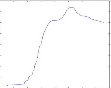
To gain some insights in the nonlinearity of the S&P 500 we plot in Figure 2 the …tted regression from
Yt=c1cos 0:5 2 2(Yt 1) +c2cos 1:5 2 2(Yt 1) +"t: (8)
We plot the least squares …tted values Ybt from the previous regression against the lagged values of Yt 1: Figure 2 reveals that the conditional mean at lag one of the S&P 500 is nonlinear and
non-decreasing around zero, a feature which is consistent with the well-known fact that the sample autocorrelation at lag j= 1 of stock returns is usually positive. We observe an asymmetric e¤ect in the …tted conditional mean with variations in negative values of Yt 1 larger than variations in
positive values. This is consistent with the well-known “Leverage e¤ect”in stocks returns, in which volatility is higher when past stock returns are negative. The positive correlation e¤ect is reversed for “large” absolute values of the returns. More concretly, for values larger than 1:2 the …tted regression is decreasing, re‡ecting the expectations of investors that after a large positive return foresee a decay in the stock price return.
— — — — — — — — — — — FIGURE 2 ABOUT HERE
— — — — — — — — — — —
6
Extensions, modi…cations and conclusions
This section discusses extensions and modi…cations of the basic setup considered in the paper. The major limitation of the proposed methodology is that tests based on Rn in (2) only have power against alternatives satisfyingE[Yt1(Yt 1 x)]6= 0in a set with positive Lebesgue measure. These
alternatives correspond to those such thatE[YtjYt 1]6= 0:The motivation for the use of justYt 1
as the conditioning variable is practical, one expects that the most important lag is the …rst one in real data, but mostly theoretical, since the principal components and eigenvalues associated toRn are only known for this univariate case.
Here, we discuss two alternatives for applying the methodology of this paper to a more general multivariate case. We can consider the situation where the conditioning set is ad variate random vector, sayXt= (Yt;Z0t; ; :::; Yt P+1;Z0t P+1)0whereZtis a vector of explanatory random variables, and the mean ofYtis di¤erent from zero. That is, we are now concerned with testing the hypothesis
H0 :E[YtjXt 1] = a:s: 2R: (9)
This is the set-up considered in Domínguez and Lobato (2003).
com-ponents of the marked empirical process Rn;w(x) :=n 1=2 n X t=1 (Yt Y)w(Xt 1;x) x2Rd;
for a suitable weight functionwand where Y is the usual sample mean. See Escanciano (2006) for possible functions w: The principal components of Rn;w can be estimated consistently along the lines suggested in Escanciano (2005) by solving the eigenvalues and eigenvectors of ann nmatrix.
The second possibility is based on a marked process based on projections
Rn;ind( 0; x) :=n 1=2
n X t=1
(Yt Y)1( 00Xt 1 x) x2R:
The direction of projection 0 can be computed from projection pursuit techniques (c.f. Huber 1985) or from dimension reduction techniques as in Cook and Li (2002). Although, how to choose the projection direction is important, it will not be discussed here for the sake of space. In the context of Generelized Linear models, Stute, Presedo-Quindimil, González-Manteiga and Koul (2006) advocate for the use ofRn;ind( n; x);with nan estimator of the Generalized Linear model parameter. Here we assume that if 0is unknown, it can be estimated by apn consistent estimator
n;without restricting ourselves to a particular estimator.
As shown by Stute et al. (2006), under mild conditions, it follows that
sup
x2Rj
Rn;ind( n; x) Rn;ind( 0; x)j
P
!0:
Moreover, the asymptotic distribution ofRn;ind( n; u) underH0 is a Gaussian process with
covari-ance function
K(x1; x2) =E[(Yt )2 1( 00Xt 1 x1) F 0(x1) 1(
0
0Xt 1 x2) F 0(x2) ]; whereF 0 is the cdf of 00Xt 1:
Let ( ) be the function de…ned by
(u) = u Z 1 2 0(x)F 0(dx); with 2 0(x) :=E (Yt ) 2
j 00Xt 1 =x the conditional variance. We shall transform the limit
process ofRn;ind( n; u)to a Brownian motion in proper time. It is not only the asymptotic distrib-ution freeness of the transformation which makes this approach attractive. Rather the transformed process may be used to construct smooth tests through a principal component decomposition as
discussed above. Let A(u) := 1 Z u 2 0(x)F 0(dx):
Assume throughout that A(u)6= 0 8u2R;and consider the linear operatorT( )de…ned by
T f(u) :=f(u) u Z 1 A 1(x) 1 Z x 2 0(y)f(dy)F 0(dx);
wheref( )is either of bounded total variation or a Brownian motion B . In the latter case, the integral needs to be interpreted as a stochastic integral. Such transformations have been considered in the goodness-of-…t literature by Khmaladze (1981, 1988), see also Koul and Stute (1999), Stute and Zhu (2002) and Delgado, Hidalgo and Velasco (2005), among others. Note thatT( ) depends on unknown quantities. A natural estimator ofT( ) is
Tnf(u) =f(u) u Z 1 An1(x) 1 Z x 2 n; n(y)f(dy)Fn; n(dx); where An(u) = 1 Z u 2 n; n(x)Fn; n(dx); and n;2
n(x)is any nonparametric consistent estimator of the conditional variance, e.g. a
Nadaraya-Watson estimator. Then the transformed process can be written as
TnRn;ind( n; u) = Rn;ind( n; u) 1 n3=2 n X t=1 n X s=1 1( n0Xt 1 u)An1( 0nXt 1) 1( 0nXt 1 0nXs 1)(Ys Y) n;2n( 0nXs 1):
It can be shown that under the null hypothesisH0 and some mild conditions, including that 2n;
n
is a uniformly consistent estimator of 2
0;we have that
TnRn;ind( n; u) =)B (u) inD([ 1;1)):
See Stute, Thies and Zhu (1998).
In particular from the scaling properties of the Brownian motion and the Continuous Mapping Theorem we have that
a Z 1 1 n (a)TnRn;ind( n; x) 2 n(dx) d ! 1 Z 0 jB(u)j2du; (10)
where n(x) =n 1 n X t=1 (Yt Y)21( 0nXt 1 x):
At this point, the data-driven smooth test can be computed in exactly the same manner as in Section 3. Formal details are omitted for the sake of space.
Now, we discuss di¤erent selection rules for the data-driven smooth test. In this paper we have adopted the combination rule of Inglot and Ledwina (2006a), but other rules are available in the literature. See the aforementioned references. Among other rules, the most popular choice in the context of smooth tests is the Schwarz’s selection rule of Ledwina (1994). This corresponds to
mBIC = minfm: 1 m d;Lm Lh; h= 1;2:::; dg;
where
Lm=Tn;m mlogn:
Also other choices of q in our combination rule can be considered. Inglot and Ledwina (2006b) provided simulations with di¤erent choices of q for data-driven smooth tests for testing uniformity in the context of goodness-of-…t tests for distributions. Here we run a small Monte Carlo experiment and consider the AR(1)-GARCH(1,1) model as in the Monte Carlo section forc= 0:1;0and 0:1. We recall that small values of q in the combination rule results in the Akaike’s criterion, while large q0s lead to the choice of the Schwarz’s criterion. This is con…rmed in the simulations. In Table 6 we report the empirical rejection probabilities for the AR(1)-GARCH(1,1) model. Tn;mBIC
stands for the data-driven smooth test with the Schwarz’s selection rule whereas Tn;me(q) denotes the data-driven test with our combination rule using q: We observe that di¤erent values of q lead to small variations in the rejection probabilities.
— — — — — — — — — — — TABLE 6 ABOUT HERE
— — — — — — — — — — —
To conclude, we have proposed a new data-driven smooth test for the MDH with excellent power properties, comparing well to other competing tests. Theoretical results such as the lack of power of omnibus tests or the inability of the t test to detect certain nonlinear alternatives have been con…rmed also empirically. The new smooth tests provide a compromise between the omnibus tests, which are consistent against all alternatives, and directional tests, which are optimal in a given (unique) univariate direction. Optimality, in a semiparametric sense, of our test has been shown for a class of Markov processes. We have demonstrated that high-frequency alternatives are likely to appear in …nancial applications. Our data-driven smooth tests are especially convenient to
detect such alternatives, while being able to detect also low-frequency alternatives. An important extension of our tests would be to consider the bounddtending to in…nity with the sample size. This extension is di¢ culted by the general serial dependence allowed in our framework. It is expected that under suitable mixing conditions such an extension can be accomplished. This challenging problem is deferred for future research.
7
Appendix: Mathematical Proofs
Proof of Theorem 1: The proof follows easily from Lemma 2 in Domínguez and Lobato (2004),
and hence, it is omitted.
Proof of Theorem 2: (i) The Uniform Ergodic Theorem, see e.g. Dehling and Philipp (2002),
and A1 yield
sup
x2R 2
n(x) 2(x) =oP(1):
The last display, Theorem 1 and Lemma 3.1 in Chang (1990) imply, for 1 j d;
bj;n = j1=2
Z R
j( 2(x))Rn(x) 2(dx) +oP(1)
: =ej;n+oP(1); whereej;n can be written as
ej;n := p 2 1=2 j pn n X s=1 Yscos((j 1=2) 2 2(Ys 1)): (11)
Notice that,E[ej;n] = 0and E[ej;neh;n] = 2
Z R
cos((j 1=2) 2(x)) cos((j 1=2) 2(x)) 2(dx)
= jh;
where jh = 0 ifj6=h, and jh = 1 otherwise.
Now, by the Cramer-Wold device, A1 and the Central Limit Theorem (CLT) for martin-gales with stationary and ergodic di¤erences (Billingsley (1961)) it readily follows that the vector
(e1;n; :::;em;n)0 converges to a m variate standard normal random vector. This implies part (i). As for part (ii). Denote the Schwarz’s rule for the choice ofm by
where
Lm=Tn;m mlogn:
We shall prove that under H0;me =mBIC with probability tending to one. To that end, de…ne the event
An(q) = max
1 j djbj;nj> p
qlogn :
From part (i) we have that max
1 j djbj;nj =OP(1): Thus, it follows that P(An(q)) = o(1); which in turn implies limn!1P(me =mBIC) = 1:
Now, we prove that, again underH0;
lim
n!1P(mBIC= 1) = 1: (12)
First, notice that
P(mBIC = 1) = 1 d X j=1 P(mBIC =j) 1 d X j=1 P(Lj L1): (13) Now,
P(Lj L1) P(Tn;j (j 1) log(n)) Cn ; for some >0;
where the last inequality follows from the moderate deviation inequality for multivariate martingales in Grama and Haeusler (2006), see their Theorem 2 and Corollary 1. Therefore, Theorem 2 follows from (12) and application of the standard CLT for martingales. The theorem is proved.
Before proving Theorem 3 we need some notation and discussion. We proceed to investigate the Pitman asymptotic relative e¢ ciency of tests in this semiparametric testing environment, along the lines of Choi, Hall, and Schick (1996). Write ("; X)0 for a r.v. with the same distribution as ("t; Yt 1)0: Y has also the same distribution as X: Similarly, Z denotes a r.v. with the same
probability distribution, sayP;asZt= (Yt; Yt 1)0; t2Z:LetL2(P)be the space of square integrable
random vectors with respect toP and letjj jj2;P jj jj2 indicate theL2(P)norm. Likewise, de…ne
L2(Pn) and jj jj2;Pn, where Pn is the empirical probability measure of fZtg
n
t=1: Finally, let P be
the set of probability measures forP for which the regularity conditions below hold.
The nuisance parameters in the model (7) are given by 0= (f"jX( ); f( ))0;wheref"jX( )is the conditional density of errors "given X; and f( ) is the density of X: The parameter of interest is
c 2 Rm: Let 0 = (0; 0) and = (c; ) with = (h"jX( ); h( ))0 2 H = B1 B2: Here B1 is the
set of all conditional error densities consistent with the model (7) andB2 is the set of all densities
for X; in both cases the densities are dominated by a particular -…nite measure . De…ne the densities
and consider the family of probabilities: P~ :=fP 2 P :dP=d =g(y; x;c; ), withR "h"jx("jx)d"=
0g: The family fP 2 P~ : dP=d = g(y; x;0; )g represents the space of models under the null hypothesis: Then the whole class of semiparametric models under consideration are characterized by the family of distributions
fP 2P~:dP=d =g(y; x;c; );(c; )2Rm Hg:
The construction of the e¢ cient score test proceeds as follows. Given the score _l1 in the marginal
familyP1 =fP 2P~ :dP=d =g(y; x;c; 0); c 2Rmg;one computes the tangent spaceP_2 of the
nuisance parameter family P2 =fP 2P~ :dP=d =g(y; x;0; ); 2 Hg. Then the e¢ cient score
l1 can be constructed by the orthogonal projection of score _l1 on the orthocomplement of P_2; i.e.,
l1 =_l1 [_l1jP_2]; where [hjP_2]denotes the orthogonal projection in L2(P) of h on P_2:A score
test using the e¢ cient score along this least favorable direction will be anasymptotically uniformly most powerful invariant and asymptotically unbiased test at 0; in short AUMPIU ( ; 0), as de…ned in Choi, Hall, and Schick (1996). Eventually it turns out that the test does not depend on
0;extending its uniformity over all alternatives with di¤erent 0’s. In this case, we say that the
test is AUMPIU( ).
Wefelmeyer (1997) characterized the tangent space P_2 of the nuisance parameter family P2:
The tangent space P_2 atP 2 P2 is given by
_
P2 =fs2L2(P) :E[s(Z)] = 0; E[Ys(Z)jX] =0g:
The following lemma establishes the projection operator [hjP_2]:
Lemma A1: Under Assumptions A1-A2,P_2 is the tangent space of the nuisance parameter family
P2;and
[sjP_2](z) =s(z) E[s(Z)] y 2(x)E[Ys(Z)jX =x]; fors2L2(P); z= (y; x):
Proof of Lemma 1: That P_2 is the tangent space of the nuisance parameter family P2 follows
from Wefelmeyer (1997). For the rest of the proof it su¢ ces to show that (a) [sjP_2]2 P_2 and
(b) s [sjP_2] ? P_2: To show (a), notice that using the null restriction E[YjX] = 0; we have
E( [hjP_2]) = 0:Also
E[Y [sjP_2]jX] = E[Ys(Z)jX] E[Ys(Z)jX=x]
Hence (a) is proved. To show (b), notice that fors2P_2;
E[ h [hjP_2] s(Z)] = E[Y 2(X)E[Yh(Z)jX =x]s(Z)]
= 0:
Proof of Theorem 3: The marginal score _l1 is given by
_l1(z) = h(x)l"=x(z);
wherel"=x(z) :=@lnf"=x(z)=@":Notice that E[l"=x(Z)Y jX] = 1:Hence,
l1 = _l1 [_l1jP_2]
= y 2(x)E[Y_l1(Z)jX=x]
= y 2(x)h(x):
An optimal (semiparametric) score test rejects the null hypothesis H0 for large values of
Tn;e(a) = ( 1 p n n X t=1 l1(Zt) )0 I 1 ( 1 p n n X t=1 l1(Zt) ) ;
where I: = jjl1(Zt; a)jj2;P: Similar arguments to those of Theorem 2 show that I is the identity matrix of order mand that
Tn;e(a) = m X j=1 (ej;n)2= m X j=1 b2j;n+oP(1);
whereej;n is de…ned in (11). We have shown that the test based on Tn;e(a) is AUMPIU( ) for testing Hs0 :c=0 againstHs1 :c6=0:
REFERENCES
Aerts, M., Claeskens, G. and Hart, J. D. (1999), “Testing Lack of Fit in Multiple Regression,”
Journal of the American Statistical Association,94, 869-879.
Bickel, P. J. , A.J. Klaassen, Y. Rikov, and J. A. Wellner (1993), E¢ cient and Adaptive Esti-mation for Semiparametric Models. Springer Verlag, New York.
Billingsley, P. (1961), “The Lindeberg-Levy Theorem for Martingales,”Proceedings of the Amer-ican Mathematical Society,12, 788-792.
Bosq, D. (2000),Linear Processes in Function Spaces. Theory and Applications. Springer, New York.
Box, G., and Pierce, D. (1970), “Distribution of Residual Autocorrelations in Autorregressive Integrated Moving Average Time Series Models,”Journal of American Statistical Association,65, 1509-1527.
Chang, N. M. (1990), “Weak Convergence of a Self-Consistent Estimator of a Survival Function with Doubly Censored Data,”Annals of Statistics, 18, 391-404.
Choi, S., W. J. Hall, and A. Schick (1996), “Asymptotically Uniformly Most Powerful Tests in Parametric and Semiparametric Models,”Annals of Statistics, 24, 841-861.
Cochrane, J. (2001), Asset Pricing. Princeton University Press. Princeton, New Jersey.
Cook, R.D., and Li, B. (2002), “Dimension Reduction for Conditional Mean in Regression,”
Annals of Statistics, 30, 455-474.
Dehling, H., and Philipp, W. (2002), “Empirical Process Techniques for Dependent Data,” In
Empirical processes techniques for dependent data. H. Dehling, T. Mikosch and M. Sorensen (Eds.). Birkhauser Boston, p. 1-115, 2002.
Delgado, M. A., Hidalgo, J. and Velasco, C. (2005), “Distribution Free Goodness-of-…t Tests for Linear Models,”Annals of Statistics, 33, 2568-2609.
Deo, R. S. (2000), “Spectral Tests of the Martingale Hypothesis under Conditional Heteroskedas-ticity,”Journal of Econometrics,99, 291-315.
Dominguez, M. A and Lobato, I. N. (2003), “A Consistent Test for the Martingale Di¤erence Hypothesis,”Econometric Reviews, 22, 351-377.
Durbin, J. and Knott, M. (1972), “Components of Cramer-von Mises Statistics. I,”Journal of the Royal Statistical Society. Ser. B, 34, 290-307.
Durlauf, S. (1991), “Spectral Based Testing of the Martingale Hypothesis,” Journal of Econo-metrics, 50, 355-376.
Escanciano, J. C. (2006), “Goodness-of-Fit Tests for Linear and Non-Linear Time Series Mod-els,”Journal of the American Statistical Association, 101, 531-541.
Escanciano, J. C. (2005), “On The Asymptotic Power Properties of Speci…cation Tests for Dynamic Parametric Regressions,” Working paper 07/05 Universidad de Navarra.
Escanciano, J. C., and Velasco, C. (2006), “Generalized Spectral Tests for the Martingale Dif-ference Hypothesis,”Journal of Econometrics,134, 151-185.
Statistics,27, 747-763.
Eubank, R.L. and LaRiccia, V.M. (1992), “Asymptotic Comparison of Cramer-von Mises and Nonparametric Function Estimation Techniques for Testing Goodness-of-Fit,”Annals of Statistics,
20, 2071-2086.
Eubank, R., and Hart, J. (1992), “Testing Goodness-of-Fit in Regression via Order Selection Criteria,”Annals of Statistics,20, 1412-1425.
Fan, J. (1996), “Test of Signi…cance Based on Wavelet Thresholding and Neyman’s Truncation,”
Journal of the American Statistical Association,91, 674-688.
Fan, J. and Huang, L. (2001), “Goodness-of-Fit Tests for Parametric Regression Models,” Jour-nal of the American Statistical Association, 96, 640-652.
Gallant, A. R., Hsieh, D. A. and Tauchen, G. (1991), “On Fitting a Recalcitrant Series: The Pound/Dollar Exchange Rate, 1974-1983,” in Nonparametric and Semiparametric Methods in Econometrics and Statistics. Eds. W. A. Barnett, J. Powell and G. Tauchen, Cambridge, U.K. Cambridge University Press, 199-240.
Grama, I. G., and Haeusler, E. (2006), “An Asymptotic Expansion for Probabilities of Moderate Deviations for Multivariate Martingales,”Journal of Theoretical Probability, 19, 1-44.
Hall, P., and Heyde, C. C. (1980), Martingale Limit Theory and Its Application. Academic Press, New York.
Hsieh, D. A. (1989), “Testing for Nonlinear Dependence in Daily Foreign Exchange Rates,”
Journal of Business,62, 339-368.
Huber, P. J. (1985), “Projection Pursuit (with discussion),”Annals of Statistics, 13, 435-525. Inglot, T. and Ledwina, T. (1996), “Asymptotic Optimality of Data-Driven Neyman’s tests for Uniformity,”Annals of Statistics, 24, 1982-2019.
Inglot, T. and Ledwina, T. (2006a), “Towards Data Driven Selection of a Penalty Function for Data Driven Neyman Tests,”Linear Algebra and its Applications, 417, 124-133.
Inglot, T. and Ledwina, T. (2006b), “Data Driven Score Tests of Fit for Semiparametric Ho-moscedastic Linear Regression Model”, Preprint 665, Institute of Mathematics Polish Academy of Sciences.
Kallemberg, W. C. M. (2002), “The Penalty in Data Driven Neyman’s Tests,”Mathematical Methods of Statistics, 11, 323-340.
Kallenberg, W. C. M. and Ledwina, T. (1997), “Data-Driven Smooth Tests When the Hypoth-esis is Composite,”Journal of the American Statistical Association,92, 1094-1104.
Khmaladze, E.V. (1981), “Martingale Approach in the Theory of Goodness-of-Fit Tests,” The-ory of Probability and its Applications, 26, 240-257.
Khmaladze, E.V. (1988), “An Innovation Approach to Goodness-of-Fit Tests in Rm,”Annals of Statistics, 16, 1503-1516.
Koul, H. L. and Stute W. (1999), “Nonparametric Model Checks for Time Series,”Annals of Statistics,27, 204-236.
Koziol, J. A. (1980), “On a Cramer-von Mises-Type Statistic for Testing Symmetry,”Journal of the American Statistical Association,75, 161-167.
Janssen, A. (2000), “Global Power Functions of Goodness of Fit Tests,”Annals of Statistics,
28, 239-253.
Ledwina, T. (1994), “Data-Driven Version of Neyman’s Smooth Test of Fit,”Journal of the American Statistical Association, 89, 1000-1005.
Neyman, J. (1937), “Smooth Test for Goodness of Fit,”Scandinavian Aktuarietidskr,20, 149-199.
Rayner, J. C. W., and Best, D. J. (1989), Smooth Tests of Goodness of Fit. London: Oxford University Press.
Stute, W., Presedo Quindimil, M., Gonzalez Manteiga, W. and Koul, H. L. (2006), “Model Checks of Higher Order Time Series,”Statistica Sinica, forthcoming.
Stute, W., Thies, S., and Zhu, L.X. (1998), “Model Checks for Regression: an Innovation Process Approach,”Annals of Statistics, 26, 1916-1934.
Stute, W. and Zhu, L. X. (2002), “Model Checks for Generalized Linear Models,”Scandinavian Journal of Statistics, 29, 535-545.
Wefelmeyer, W. (1997), “Adaptive Estimators for Parameters of the Autoregression Function of a Markov Chain,”Journal of Statistical Planning and Inference,58, 389-398.
Figure 1: Size and Power of Tests at 5% for the model (1-2) -0.2 -0.1 0 0.1 0.2 0 0.2 0.4 0.6 0.8 1 c Re je c tio n P ro b a b ili tie s Garch(1,1), n=500 -0.2 -0.1 0 0.1 0.2 0 0.2 0.4 0.6 0.8 1 c Re je c tio n P ro b a b ili tie s Garch(1,1), n=1000 -0.2 -0.1 0 0.1 0.2 0 0.2 0.4 0.6 0.8 1 c Re je c tio n P ro b a b ili tie s EGarch(1,1), n=500 -0.2 -0.1 0 0.1 0.2 0 0.2 0.4 0.6 0.8 1 c Re je c tio n P ro b a b ili tie s EGarch(1,1), n=1000
KS-dash, CvM-square, t-test–plus, Tn;me-start,Tn;3-circle. 5%level, sample size n= 500 and
n= 1000:Innovations distributed as N(0;1).
Table 1: Power and Size of Tests at 5%for the model 3.
n=500 c= 0:6 c= 0:3 c= 0:0 c= 0:3 c= 0:6 j= 2 j= 3 j = 2 j= 3 j= 2 j= 3 j= 2 j = 3 j= 2 j= 3 KS 0:123 0:059 0:077 0:067 0:038 0:036 0:067 0:052 0:131 0:058 CvM 0:067 0:042 0:068 0:070 0:039 0:044 0:062 0:048 0:068 0:038 t test 0:058 0:042 0:051 0:049 0:035 0:060 0:047 0:048 0:038 0:047 Tn;3 0:179 0:056 0:095 0:063 0:051 0:038 0:094 0:058 0:155 0:053 Tn;me 0:989 0:858 0:273 0:191 0:051 0:060 0:287 0:192 0:993 0:871
Table 2: Power of Tests at 5%for the model NLMA n= 300 n= 500 KS 0.039 0.074 CvM 0.042 0.051 t test 0.065 0.073 Tn;3 0.480 0.642 Tn;me 0.781 0.755
Table 3: Summary statistics of the returns
n=755 S&P500 AF BA Cit Ea Ec Ex GE GM Pep Sta Mean -0.042 -0.269 -0.036 -0.039 -0.069 -0.052 -0.061 -0.043 0.091 -0.039 -0.137 Median -0.071 0.013 -0.059 -0.025 -0.089 0.000 -0.150 0.000 0.129 -0.035 -0.031 SD 0.821 1.716 0.997 1.144 1.420 1.145 1.199 1.165 2.004 1.379 1.631 Skew. -0.100 -0.768 1.800 -0.079 0.074 -0.201 0.339 -0.255 -0.045 0.028 -0.727 Kurt. 4.234 4.766 20.318 4.378 5.164 3.484 3.912 4.413 14.932 12.420 11.246 Maxi. 3.587 3.123 10.677 4.116 7.677 3.252 4.455 4.642 15.045 10.234 8.560 Minim. -3.481 -6.518 -2.654 -5.320 -5.808 -5.103 -3.677 -5.756 -16.647 -9.481 -13.659
Table 4: p-values of the tests. S&P 500 and some of its components.
S&P500 AF BA Cit Ea Ec Ex GE GM Pep Sta
KS 0.136 0.150 0.299 0.424 0.088 0.170 0.170 0.597 0.256 0.299 0.038
CvM 0.113 0.136 0.248 0.447 0.127 0.137 0.166 0.566 0.227 0.248 0.103
t test 0.045 0.462 0.285 0.624 0.788 0.000 0.299 0.700 0.745 0.395 0.057 Tn;3 0.000 0.405 0.012 0.227 0.004 0.000 0.000 0.699 0.406 0.001 0.018
Tn;me 0.000 0.000 0.000 0.571 0.004 0.000 0.000 0.528 0.000 0.000 0.000
Table 5: Individual Principal Components. S&P 500 and some of its components.
S&P500 AF BA Cit Ea Ec Ex GE GM Pep Sta
e
m(10) 2 10 10 1 2 2 2 1 10 2 10
b2me(10);n 22.95 9.05 81.10 0.32 6.73 20.39 16.29 0.39 27.97 15.14 30.51 Note: * Signi…cative at 5%, ** Signi…cative at 1%.
Figure 2: Fitted model (8) for S&P 500 -4 -3 -2 -1 0 1 2 3 4 -3 -2.5 -2 -1.5 -1 -0.5 0 0.5 1 Y (t-1)
Alternativ e model f or S&P 500
Table 6: GARCH(1,1) Gaussian-errors, n =500
c= 0:1 c=0 c=0:1 Tn;mBIC 0.259 0.060 0.273 Tn;me(2:2) 0.267 0.067 0.279 Tn;me(2:4) 0.264 0.064 0.277 Tn;me(2:6) 0.264 0.063 0.276 Tn;me(2:8) 0.264 0.062 0.276 Tn;me(3) 0.262 0.061 0.275 Tn;me(3:2) 0.261 0.060 0.274