ENERGY CONSUMPTION AND ECONOMIC GROWTH IN BOTSWANA: EMPIRICAL EVIDENCE FROM A DISAGGREGATED DATA
Forthcoming: International Review of Applied Economics
Nicholas M. Odhiambo Working Paper 12/2020
July 2020 Nicholas M. Odhiambo Department of Economics University of South Africa P. O. Box 392, UNISA
0003, Pretoria South Africa
Emails: odhianm@unisa.ac.za / nmbaya99@yahoo.com
UNISA Economic Research Working Papers constitute work in progress. They are papers under submission or forthcoming elsewhere. The views expressed in this paper, as well as any errors or omissions are, therefore, entirely those of the author(s). Comments or questions about this paper should be sent directly to the corresponding author.
©2019 by Nicholas M. Odhiambo
UNISA ECONOMIC RESEARCH
WORKING PAPER SERIES
2
ENERGY CONSUMPTION AND ECONOMIC GROWTH IN BOTSWANA: EMPIRICAL EVIDENCE FROM A DISAGGREGATED DATA
Nicholas M. Odhiambo Abstract
In this paper we examine the causal relationship between energy consumption and economic growth in Botswana during the period 1980-2016. We disaggregate energy consumption into six components, namely: total energy consumption, electricity consumption, motor gasoline, gas/diesel oil, fuel oil and liquefied petroleum gas. We then compare the results of the disaggregated energy components with that of the aggregated energy consumption level. In order to account for the omission-of-variable bias, we incorporate inflation and trade openness as intermittent variables between the various components of energy consumption and economic growth, thereby creating a system of multivariate equations. Using the ARDL-bound testing approach, the study found a causal flow from economic growth to energy consumption to predominate. This finding has important policy implications as it shows that the buoyant economic growth that Botswana has enjoyed over the years is not energy-dependent, and that the country could pursue the requisite energy conservation policies without necessarily stifling its economic growth. To our knowledge, this study may be the first of its kind to examine in detail the causal relationship between energy consumption and economic growth in Botswana using a multivarite causality model and a disaggregated dataset.
Keywords: Botswana, Disaggregated Energy Consumption, Economic Growth, ARDL-bounds Testing Approach
1. Introduction
The dynamic causal relationship between energy consumption and economic growth has attracted considerable amount of attention in recent years. Theoretically, energy can be regarded as a driver of economic growth because it is one of the key factors of pro-duction, along with capital and labour (see Abosedra et al, 2015). According to Razzaqi (2011), energy is an essential input for growth and development. Likewise, energy use can also be a limiting factor to economic growth, since other factors of production
3
cannot work properly without it. Studies have also shown that the effect of energy use on economic growth depends largely on the structure of the economy’s energy intensity, as well as the stage of that country’s economic growth (see Razzaqi 2011: 438). Although early growth models did not explicitly include energy as one of the factors of production, the role of energy in the production process has recently been recognised in the light of the endogenous growth model. Indeed, the increasing role of energy in the production process has led to the incorporation of energy as an input in the production process by many studies. Recent studies have also linked energy to the environmental Kuznets curve theory, developed by Grossman and Krueger (1991). This is because many studies have found that energy plays a crucial role in estimating the turning points of the inverted U-shape relationship between economic growth and environmental quality – popularly known as the environmental Kuznets curve (see Mandal and Chakravarty, 2017). On the empirical front, the relationship between energy consumption and economic growth has been at best inconclusive. While some studies have maintained that there is a unidirectional causality from energy consumption to economic growth, others have argued that it is economic growth that Granger-causes energy consumption. Between these two extremes, there are other stu-dies arguing that there is a bidirectional causal relationship between energy consump-tion and economic growth. While the majority of the previous studies confirm the existence of a causal relationship between energy consumption and economic growth, there is a fourth view called ‘neutrality hypothesis’, which argues that there is no causality in either direction between energy consumption and economic growth. Although a number of studies have been conducted on the causal relationship between energy consumption and economic growth in various countries, very few country-based studies have been conducted on African countries. In fact, the majority of the previous studies have mainly concentrated on Asia and the Latin American countries. Studies on sub-Saharan African countries, such as Botswana, are therefore difficult to come by.
It is also worth mentioning that even where such studies have been conducted, the empirical findings are inconclusive in the main. They differ from country to country and over time, as well as the proxy used to measure the level of energy consumption (see Odhiambo, 2009a; 2010). Some of the previous studies have also been found to suffer from a number of methodological weaknesses. For example, some studies used cross-sectional data, which have been found to be unreliable as data lumped together
4
from different countries may not satisfactorily address country-specific issues. The weakness of using the cross-sectional data method has been extensively discussed in the literature (see, for example, Ghirmay, 2004; Quah, 1993; Casselli et al., 1996; Odhiambo, 2008; and Odhiambo, 2010, among others). The other weakness of some of the previous studies hinges on the use of a bivariable causality model, which has been found to suffer from the omission-of-variable bias. Previous studies have found that the introduction of an additional variable in a bivariate setting is likely to change not only the magnitude of the empirical results, but also change the direction of causality between the two studied variables.
The current study, therefore, examines the causal relationship between energy consumption and economic growth in Botswana using disaggregated data for the period 1980-2016. The study aims to answer two critical questions: 1) Is economic growth in Botswana energy-dependent? 2) Which components of energy demand drive economic growth in Botswana? In order to answer these two critical questions, we disaggregate energy consumption into six components, namely: total energy consumption, electricity consumption, motor gasoline, gas/diesel oil, fuel oil and liquefied petroleum gas. We then compare the results of the disaggregated energy components with that of the aggregated energy consumption level. In order to account for the omission-of-variable bias, we incorporate inflation and trade openness as intermittent variables between the various components of energy consumption and economic growth – thereby creating a system of multivariate equations. To our knowledge, this study may be the first of its kind to examine in detail the relationship between energy consumption and economic growth in Botswana using a multivariate ECM-based Granger causality model and a disaggregated dataset.
The rest of the paper is structured as follows: Section 2 gives an overview of energy consumption and economic growth in Botswana. Section 3 deals with the literature review, while section 4 presents the empirical model specification, the estimation techniques and the empirical analysis of the regression results. Section 5 concludes the study.
5
2. Energy Consumption and Economic Growth in Botswana
Botswana’s energy components mainly comprise electricity, wood fuel, liquefied petroleum gas, (LPG), petrol, diesel and aviation gas. Due to the increase in electrification over the years, the use of wood fuel has shown a downward trend in recent years. On the other hand, the use of electricity and liquefied petroleum gas has shown an upward trend. The total electricity consumption, for example, increased from 0.99 Twh in 1990 to 1.90 Twh in 2000, and later to 3.79 Twh in 2004. The consumption of liquefied petroleum gas (LPG), on the other hand, increased from 11 kt in 1990 to 20 kt in 2000, and later to 26 kt in 2014 (see IEA, 2016). Despite the significant increase in electrification, wood fuel still remains the main energy source for cooking, especially in rural households. Botswana’s power sector has been dominated by coal, which accounts for about 82% of the country’s total power production (see Climate Scope, 2016). Although Botswana has an abundance of energy sources, the country in part relies on energy imported from South Africa and Mozambique. For example, in 2011, it is estimated that about 66% of Botswana’s electricity demand was sourced from South Africa, while another 22% was sourced from Mozambique. It is projected that the peak prior demand will increase to 902 MW by 2020 from 578 MW in 2012 (see REEP, 2014). Botswana’s electrification rate is very impressive when compared with some African countries. For example, by 2012, about 58% of the country’s population had access to grid electricity services. Botswana energy policy has over the years been guided by the country’s Vision 2016, Nation Energy policy and Botswana Energy Master Plan. The overall goal of the country’s National Energy Policy is to meet the energy needs of Botswana for social and economic development in a sustainable manner (see Government of the Republic of Botswana, National Energy Policy, 2009). According to Vision 2016 plan, the country’s energy target was to achieve 80% national power access and 60% rural power access by 2016 (see also REEP, 2014).
On the economic growth front, it is worth noting that Botswana is currently one of the most prosperous countries in Africa. The country grew from being one of the least-developed economies in the 1960s, to one of the middle-income economies in Africa. In fact, Botswana is currently one of the few upper middle-income countries in sub-Saharan Africa (see Odhiambo, 2013). Between 1967-2006, for example, the country’s economic growth rate averaged 9% per year. In 2007, Botswana was listed as the third
6
richest country in Africa, according to GDP per capita. The country had a GDP per capita of about US$14,700, and ranked number 74 worldwide. Although in 2009, Botswana experienced its worst recession in almost four decades, due to the global economic recession, its own recession did not last long. In 2010, the country’s real GDP growth increased to about 7%. Currently, the country is ranked number 84 worldwide – with a GDP per capita of about USD 14,000
3. Literature review
The causal relationship between energy consumption and economic growth has been examined extensively in a number of countries in recent years, with conflicting results. Three views exist regarding the relationship between energy consumption and economic growth. The first view, which posits that energy consumption Granger-causes economic growth, has been supported by studies like those of Chang et al. (2001) for the case of Taiwan; Wolde-Rufael (2004) for Shanghai; Lee (2005) for the case of developing countries; Altinay and Karagol (2005) for Turkey; Chiou-Wei et al. (2008) for Taiwan, Hong Kong, Malaysia and Indonesia; Akinlo (2009) for Nigeria; Odhiambo (2009a) for Tanzania; Odhiambo (2010) for the case of South Africa and Kenya; Chu (2012) for the case of 13 countries; Dergiades et al. (2013) for Greece; Muhammad et al. (2013) for Pakistan; Odhiambo (2014) for the case of Uruguay and Brazil; Abosedra et al. (2015) for Lebanon; Iyke (2015) for Nigeria; Tang et al. (2016) for Vietnam; Rahman (2017) for the case of Asian populous countries; Saidi et al. (2017) for the case of the European countries; Cai et al. (2018) for the case of Canada, Germany and the US; Le and Quah (2018) for the case of 14 selected countries in the Asia and the Pacific region; Bekun et al. (2019) for South Africa; and more recently Rahman et al. (2020) for the case of China when coal and oil consumption are used as proxies for energy consumption.
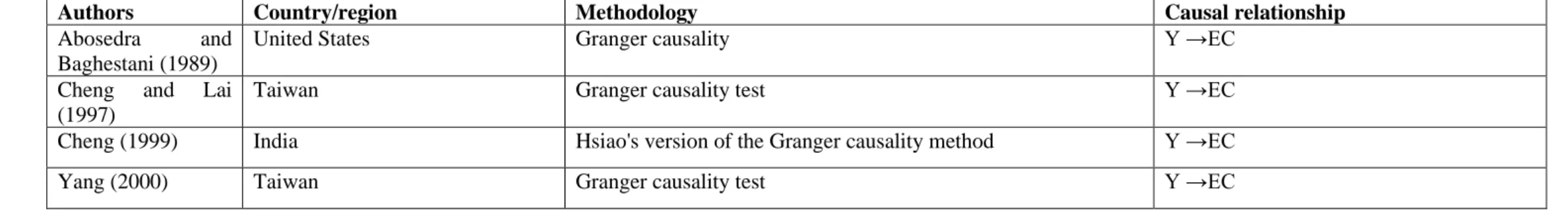
The second view, which supports growth-led energy consumption, includes studies like those by Abosedra and Baghestani (1989) for the case of the US; Cheng and Lai (1997) for Taiwan; Cheng (1999) for the case of India; Yang (2000) for Taiwan; Gosh (2002) for India; Shiu and Lam (2004) for China; Hatemi-J and Irandoust (2005) for Sweden; Narayan and Smyth (2005) for Australia; Al-Iriani (2006) for the case of the Gulf Cooperation Council (GCC) countries; Yoo and Kim (2006) for Indonesia; Chen et al. (2007) for the case of India, Malaysia, Philippines and Singapore; Mehrara (2007) for
7
the case of 11 oil-exporting countries; Mozumder and Marathe (2007) for Bangladesh; Ang (2008) for Malaysia; Chiou-Wei et al. (2008) for Philippines and Singapore for the case of nonlinear Granger causality test; Hu and Lin (2008) for Taiwan; Odhiambo (2010) for the case of the DRC; Onuonga (2012) for Kenya; Zhang and Xu(2012) for China; Ocal and Aslan (2013) for Turkey; Odhiambo (2014) for the case of Ghana and Cote d’Ivoire; Rahmad and Velayutharn (2020) for the case of South Asia; and Rahman et al. (2020) for the case of China when gas consumption is used as a proxy for energy consumption.
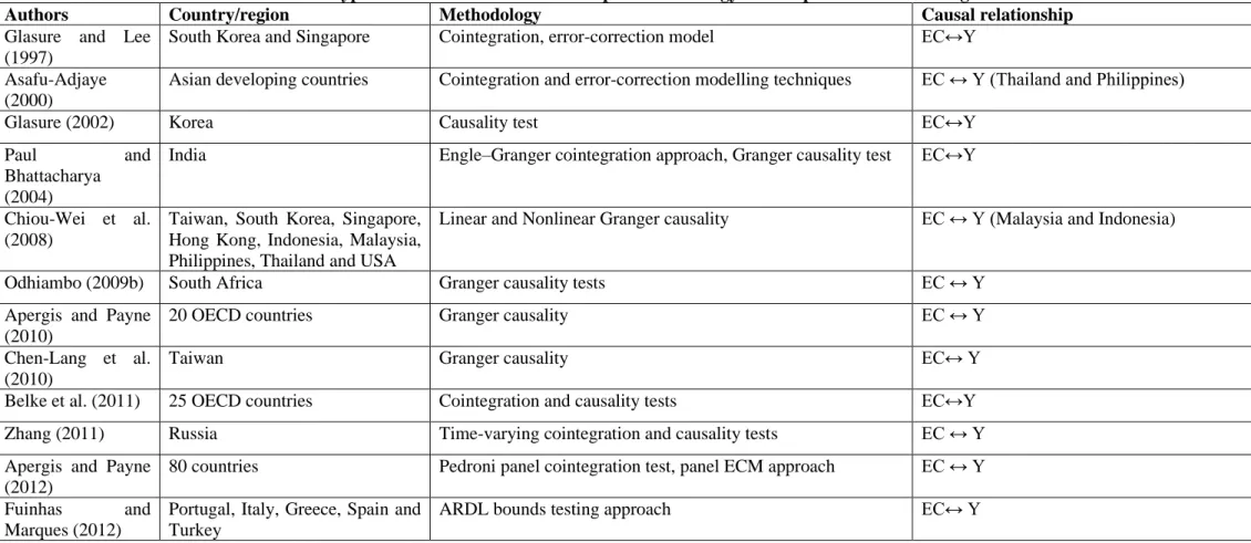
The third view, which supports a bi-directional causality between energy consumption and economic growth, includes studies such as Glasure and Lee (1997) for the case of South Korea and Singapore; Asafu-Adjaye (2000) for the case of the Philippines and Thailand; Glasure (2002) for Korea; Paul and Bhattacharya (2004) for India; Chiou-Wei et al. (2008) for Malaysia and Indonesia; Odhiambo (2009b) for South Africa; Apergis and Payne (2010) for the case of 20 OECD countries; Chen-Lang et al. (2010) for Taiwan; Belke et al. (2011) for the case of 25 OECD countries; Zhang (2011) for Russia; Apergis and Payne (2012) for the case of 80 countries; Fuinhas and Marques (2012) for the case of Portugal, Italy, Greece, Spain and Turkey; Tugcu et al. (2012) for the case of the G7 countries; Wesseh and Zoumara (2012) for Liberia; Yidirim and Aslan (2012) for the case of 17 OECD countries; Solarin and Shahbaz (2013) for Angola; Adams et al. (2016) for the case of sub-Saharan African countries; Wang et al. (2016) for China; Mirza and Kanwal (2017) for Pakistan; Saidi et al. (2017) for the case of a global panel of 53 countries; Lin and Benjamin (2018) for the case of Mexico, Indonesia, Nigeria and Turkey (MINT) countries; Eren et al. (2019) for the case of India in the long run; and Kahouli (2019) for the case of OECD countries.
The fourth view, which is also known as the neutrality view, however, argues that there is no formidable relationship between energy and economic growth, and that any perceived relationship could be merely mechanical in nature. Although this view has been somewhat unpopular, it is currently gaining traction in the empirical literature. Some studies whose findings have in one way or another supported this view include those of Altinay and Karagol (2004) for Turkey; Akinlo (2008) for Cameroon, Cote D'Ivoire, Nigeria, Kenya and Togo; Chiou-Wei et al. (2008) for South Korea, Thailand and the United States for the case of both linear and non-linear tests; Payne (2009) for
8
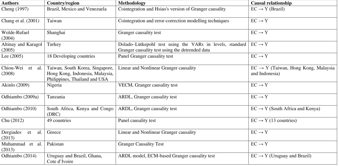
the US; Menegaki (2011) for the case of 27 European countries; Ozturk and Acaravci (2011) for most of the 11 Middle East and North Africa (MENA) countries; Chu (2012) for 24 out of 49 countries; Yildirim et al. (2014) for the case of Bangladesh, Egypt, Indonesia, Iran, Korea, Mexico, Pakistan and Philippines; Jebli and Youssef (2015) for 69 countries; Cetin (2016) for the case of E-7 Countries; Tugcu and Tiwari (2016) for BRICS; and more recently Ozcan and Ozturk (2019) for the case of sixteen (16) emerging economies. Tables 1-4 give a summary of earlier empirical findings on the causal relationship between energy and economic growth in both developed and developing countries.
9
Table 1: Studies that confirm the energy-led growth hypothesis of the causal relationship between energy consumption and economic growth
Authors Country/region Methodology Causal relationship
Cheng (1997) Brazil, Mexico and Venezuela Cointegration and Hsiao's version of Granger causality EC → Y (Brazil) Chang et al. (2001) Taiwan Cointegration and error-correction modelling techniques EC → Y
Wolde-Rufael (2004)
Shanghai Granger causality test EC → Y
Altinay and Karagol (2005)
Turkey Dolado–Lütkepohl test using the VARs in levels, standard Granger causality test using the detrended data
EC → Y
Lee (2005) 18 Developing countries Panel Granger causality test EC → Y
Chiou-Wei et al. (2008)
Taiwan, South Korea, Singapore, Hong Kong, Indonesia, Malaysia, Philippines, Thailand and USA
Linear and Nonlinear Granger causality EC → Y (Taiwan, Hong Kong, Malaysia and Indonesia)
Akinlo (2009) Nigeria VECM, Granger causality test EC → Y
Odhiambo (2009a) Tanzania ARDL, Granger causality test EC → Y
Odhiambo (2010) South Africa, Kenya and Congo (DRC)
ARDL, Granger causality test EC → Y (South Africa and Kenya)
Chu (2012) 49 countries Panel causality test EC → Y (13 countries)
Dergiades et al. (2013)
Greece Linear and Nonlinear Granger causality EC → Y
Muhammad et al. (2013)
Pakistan Granger Causality Test EC → Y
Odhiambo (2014) Uruguay and Brazil, Ghana, Cote d’Ivoire
10
Iyke (2015) Nigeria VECM, Trivariate Granger causality EC→ Y
Abosedra et al. (2015)
Lebanon VECM Granger causality EC→ Y
Tang et al. (2016) Vietnam Multivariate MWALD causality test EC → Y
Rahman (2017) Asian populous countries FMOLS–DOLS EC → Y
Saidi et al. (2017) 53 countries VECM, Granger causality test EC → Y (for the European countries)
Cai et al. (2018) G7 countries ARDL, Granger causality EC → Y (Canada, Germany and the US)
Le and Quah (2018) 14 selected countries in Asia and the Pacific
Panel Granger causality EC → Y
Bekun et al. (2019) South Africa ARDL bounds testing, Granger causality analysis EC → Y
Rahman et al. (2020) China VECM, Granger-causality tests EC → Y (for coal and oil consumption
proxies) Note: EC→Y means energy consumption causes economic growth
Table 2: Studies that confirm the growth-led energy consumption hypothesis of the causal relationship between energy consumption and economic growth
Authors Country/region Methodology Causal relationship
Abosedra and Baghestani (1989)
United States Granger causality Y →EC
Cheng and Lai (1997)
Taiwan Granger causality test Y →EC
Cheng (1999) India Hsiao's version of the Granger causality method Y →EC
11
Ghosh (2002) India Granger causality test Y → EC
Shiu and Lam (2004)
China ECK, Granger causality Y → EC
Hatemi-J and Irandoust (2005)
Sweden Causality Test Based on Bootstrap Simulation
Techniques
Y → EC Narayan and Smyth
(2005)
Australia Multivariate Granger causality test Y → EC
Al-Iriani (2006) Six Gulf Cooperation Council (GCC) countries
Panel co-integration, GMM Y → EC
Yoo and Kim (2006)
Indonesia VAR, Granger causality Y → EC
Mehrara (2007) 11 oil exporting countries Panel Granger causality Y → EC
Mozumder and Marathe (2007)
Bangladesh Cointegration test, VECM Y → EC
Ang (2008) Malaysia Granger causality Y → EC
Chiou-Wei et al. (2008)
Taiwan, South Korea, Singapore, Hong Kong, Indonesia, Malaysia, Philippines, Thailand and USA
Linear and Nonlinear Granger causality Y → EC (Philippines and Singapore – for the case of nonlinear Granger causality test)
Hu and Lin (2008) Taiwan Hansen-Seo threshold cointegration, VECM Y → EC
Odhiambo (2010) South Africa, Kenya and Congo (DRC)
ARDL, Granger causality Y →EC (Congo (DRC)
Onuonga (2012) Kenya Error Correction Model, Ganger-causality Y → EC
Zhang and Xu (2012)
China Panel Granger causality test Y → EC
Ocal and Aslan (2013)
Turkey ARDL, Toda-Yamamoto Causality Tests Y →EC
Odhiambo (2014) Uruguay and Brazil, Ghana, Cote d’Ivoire
12
Rahmad and
Velayutharn (2020)
South Asia Panel FMOLS and DOLS estimation techniques, Dumitrescu-Hurling panel causality tests
Y → EC Rahman et al.
(2020)
China VECM, Granger-causality test EC → Y (for gas consumption)
Note: Y→EC means economic growth causes energy consumption
Table 3: Studies that confirm the feedback hypothesis of the causal relationship between energy consumption and economic growth
Authors Country/region Methodology Causal relationship
Glasure and Lee (1997)
South Korea and Singapore Cointegration, error-correction model EC↔Y Asafu-Adjaye
(2000)
Asian developing countries Cointegration and error-correction modelling techniques EC ↔ Y (Thailand and Philippines)
Glasure (2002) Korea Causality test EC↔Y
Paul and
Bhattacharya (2004)
India Engle–Granger cointegration approach, Granger causality test EC↔Y
Chiou-Wei et al. (2008)
Taiwan, South Korea, Singapore, Hong Kong, Indonesia, Malaysia, Philippines, Thailand and USA
Linear and Nonlinear Granger causality EC ↔ Y (Malaysia and Indonesia)
Odhiambo (2009b) South Africa Granger causality tests EC ↔ Y
Apergis and Payne (2010)
20 OECD countries Granger causality EC ↔ Y
Chen-Lang et al. (2010)
Taiwan Granger causality EC↔ Y
Belke et al. (2011) 25 OECD countries Cointegration and causality tests EC↔Y
Zhang (2011) Russia Time-varying cointegration and causality tests EC ↔ Y
Apergis and Payne (2012)
80 countries Pedroni panel cointegration test, panel ECM approach EC ↔ Y Fuinhas and
Marques (2012)
Portugal, Italy, Greece, Spain and Turkey
13
Tugcu et al. (2012) G7 countries ARDL, Hatemi-J causality tests EC ↔Y
Wesseh and
Zoumara (2012)
Liberia Non-parametric bootstrapped causality test EC ↔Y
Yildirim and Aslan (2012)
17 OECD countries Toda Yamamoto causality test, Bootstrap-corrected causality test
EC ↔ Y Solarin and
Shahbaz (2013)
Angola VECM Granger causality EC↔ Y
Adams et al. (2016) Sub-Saharan Africa GMM panel data analysis, Panel VAR model EC ↔ Y
Wang et al. (2016) China Granger causality EC ↔ Y
Mirza and Kanwal (2017)
Pakistan ARDL–VECM EC ↔ Y
Saidi et al. (2017) 53 countries VECM, Granger causality test EC ↔ Y (Global panel)
Lin and Benjamin (2018)
Mexico, Indonesia, Nigeria and Turkey (MINT),
Panel cointegration, Panel vector error correction models EC ↔ Y (Global panel)
Eren et al. (2019) India VECM, Granger causality test EC ↔ Y
Kahouli (2019) OECD countries Pooled OLS–GLS–GMM Pooled OLS–GLS–GMM
Note: EC↔Y means there is a bidirectional causal relationship between energy consumption and economic growth
Table 4: Studies that confirm the neutrality hypothesis of the causal relationship between energy consumption and economic growth
Authors Country/region Methodology Causal relationship
Altinay and Karagol (2004)
Turkey Hsiao’s Granger-causality EC ≠ Y
Akinlo (2008) 11 African countries ARDL, Granger causality EC ≠ Y (for Cameroon, Cote D'Ivoire, Nigeria, Kenya and Togo)
Chiou-Wei et al. (2008) Taiwan, South Korea, Singapore, Hong Kong, Indonesia, Malaysia, Philippines, Thailand and USA
Linear and Nonlinear Granger causality
EC ≠ Y (South Korea, Thailand and the United States – for both the linear and nonlinear causality tests)
14
Payne (2009) US Toda-Yamamoto causality test EC ≠ Y
Menegaki (2011) 27 European countries One-way random effect model,
Panel causality test
EC ≠ Y Ozturk and Acaravci
(2011)
11 MENA countries ARDL EC ≠ Y (for most of the MENA countries)
Chu (2012) 49 countries Panel causality test EC ≠ Y (24 countries)
Yildirim et al. (2014) Bangladesh, Egypt, Indonesia, Iran, Korea, Mexico, Turkey, Pakistan and Philippines
Bootstrap autoregressive metric causality test
EC ≠ Y (Bangladesh, Egypt, Indonesia, Iran, Korea, Mexico, Pakistan and Philippines)
Jebli and Youssef (2015) 69 countries FMOLS, DOLS, VECM EC ≠Y
Cetin (2016) E-7 Countries FMOLS, DOLS, Granger causality EC ≠Y
Tugcu and Tiwari (2016) BRICS Panel bootstrap Granger causality
test
EC ≠Y
Ozcan and Ozturk (2019) 17 Emerging market economies Bootstrap panel causality test EC ≠ Y (16 emerging market economies) Note: EC ≠Y means there is no causality
15 4. Estimation techniques and empirical analysis
The ARDL bounds testing approach to cointegration
In this study, the ARDL bounds testing approach – based on the work by Pesaran and Shin (1999) and Pesaran et al (2001) – is used to examine the cointegration between the various proxies of energy consumption, economic growth, and the two intermittent variables. The advantages of using the ARDL bounds testing approach have been well documented in the literature (see also Odhiambo, 2009a). Firstly, the ARDL does not impose the restrictive assumption that all the variables included in the model must be integrated of the same order. In other words, the ARDL approach could still be applied regardless of whether the variables are integrated of order one [I(1)], order zero [I(0)] or fractionally integrated. Secondly, the ARDL technique has been found suitable even if the sample size is small. Thirdly, it has been found that the ARDL technique generally provides unbiased estimates of the long-run model and valid t-statistics even when some of the regressors are endogenous (see also Harris and Sollis, 2003). Following Pesaran et al (2001), the ARDL model used in this study can be expressed as follows:
∆𝑌/𝑁𝑡= 𝛼0+ ∑ 𝛼1𝑖∆𝑌/𝑁𝑡−𝑖+ 𝑛 𝑖=1 ∑ 𝛼2𝑖∆𝐸𝐶𝑡−𝑖+ 𝑛 𝑖=0 ∑ 𝛼3𝑖∆𝐼𝑁𝐹𝑡−𝑖+ 𝑛 𝑖=0 ∑ 𝛼4𝑖∆𝑇𝑂𝑡−𝑖 𝑛 𝑖=0 + 𝛼5𝑌/𝑁𝑡−1+ 𝛼6𝐸𝐶𝑡−1+ 𝛼7𝐼𝑁𝐹𝑡−1+ 𝛼8𝑇𝑂𝑡−1 + 𝜇1𝑡 … … … . … … … . … … (1) ∆𝐸𝐶𝑡= 𝛽0+ ∑ 𝛽1𝑖∆𝐸𝐶𝑡−𝑖+ 𝑛 𝑖=1 ∑ 𝛽2𝑖∆𝑌/𝑁𝑡−𝑖+ 𝑛 𝑖=0 ∑ 𝛽3𝑖∆𝐼𝑁𝐹𝑡−𝑖+ 𝑛 𝑖=0 ∑ 𝛽4𝑖∆𝑇𝑂𝑡−𝑖 𝑛 𝑖=0 + 𝛽5𝐸𝐶𝑡−1+ 𝛽6𝑌/𝑁𝑡−1+ 𝛽7𝐼𝑁𝐹𝑡−1+ 𝛽8𝑇𝑂𝑡−1+ 𝜇2𝑡 … . . … … (2) ∆𝐼𝑁𝐹𝑡 = 𝜋0 + ∑ 𝜋1𝑖∆𝐼𝑁𝐹𝑡−𝑖+ 𝑛 𝑖=1 ∑ 𝜋2𝑖∆𝑌/𝑁𝑡−𝑖+ 𝑛 𝑖=0 ∑ 𝜋3𝑖∆𝐸𝐶𝑡−𝑖+ 𝑛 𝑖=0 ∑ 𝜋4𝑖∆𝑇𝑂𝑡−𝑖 𝑛 𝑖=0 + 𝜋5𝐼𝑁𝐹𝑡−1+ 𝜋6𝑌/𝑁𝑡−1+ 𝜋7𝐸𝐶𝑡−1+ 𝜋8𝑇𝑂𝑡−1 + 𝜇3𝑡 … … … . . … … … (3)
16 ∆𝑇𝑂𝑡= Ω0+ ∑ Ω1𝑖∆𝑇𝑂𝑡−𝑖+ 𝑛 𝑖=1 ∑ Ω2𝑖∆𝑌/𝑁𝑡−𝑖+ 𝑛 𝑖=0 ∑ Ω3𝑖∆𝐸𝐶𝑡−𝑖 𝑛 𝑖=0 + ∑ Ω4𝑖∆𝐼𝑁𝐹𝑡−𝑖+ 𝑛 𝑖=0 Ω5𝑇𝑂𝑡−1+ Ω6 𝑌/𝑁𝑡−1+ Ω7𝐸𝐶𝑡−1 + Ω8𝐼𝑁𝐹𝑡−1 + 𝜇4𝑡 … … … . … … … (4) Where:
Y/N = Economic growth= real GDP per capita (y)
EC = Energy consumption proxies, namely: total energy consumption (Energy); liquefied petroleum gas (LPGas); motor gasoline (Mgasln); gas/diesel oil (G-Diesel); fuel oil (Fuel); and electricity (Elect);
INF = Inflation; TO = Trade openness;
𝛼0, 𝛽0, 𝜋0 and Ω0 = respective constants;
𝛼1 – 𝛼4, 𝛽 1 – 𝛽4, 𝜋1 – 𝜋4, and Ω1 – Ω4 = respective short-run coefficients;
𝛼5 – 𝛼8, 𝛽 5 – 𝛽8, 𝜋5 – 𝜋8, and Ω5 – Ω8 =respective long-run coefficients;
∆ = difference operator; n = lag length;
t = time period; and
μit= white-noise error terms.
All the data used in this study were obtained from the World Development Indicators and International Energy Agency.
Based on Pesaran et al (2001), the bounds test for the long-run relationship between the various proxies for energy consumption, economic growth and the two intermittent variables can be conducted by using the joint F-statistic (or Wald statistic) for cointegration analysis. The interpretation of the F-statistics used is based on the two sets of critical values, as recommended by Pesaran and Pesaran (1997) and Pesaran et al (2001) for a given significance level. While the first set of critical values assumes that all the variables included in the ARDL model are I(0), the second set assumes that the variables are I(1). For cointegration among the variables to hold, the computed test statistic must exceed the upper critical-bounds value. In other words, the existence of cointegration among the variables will be rejected if the F-statistic falls below the lower bounds value. However, if the computed test statistic falls between the bounds, the cointegration test is regarded as inconclusive (see also Odhiambo, 2009a; 2010).
17 ∆𝑌/𝑁𝑡= 𝛼0+ ∑ 𝛼1𝑖∆𝑌/𝑁𝑡−𝑖+ 𝑛 𝑖=1 ∑ 𝛼2𝑖∆𝐸𝐶𝑡−𝑖+ 𝑛 𝑖=1 ∑ 𝛼3𝑖∆𝐼𝑁𝐹𝑡−𝑖+ 𝑛 𝑖=1 ∑ 𝛼4𝑖∆𝑇𝑂𝑡−𝑖 𝑛 𝑖=1 + 𝛿1𝐸𝐶𝑀𝑡−1+ 𝜇1𝑡. … … … . . … … … (5) ∆𝐸𝐶𝑡 = 𝛽0+ ∑ 𝛽1𝑖∆𝐸𝐶𝑡−𝑖+ 𝑛 𝑖=1 ∑ 𝛽2𝑖∆𝑌/𝑁𝑡−𝑖 + 𝑛 𝑖=1 ∑ 𝛽3𝑖∆𝐼𝑁𝐹𝑡−𝑖+ 𝑛 𝑖=1 ∑ 𝛽4𝑖∆𝑇𝑂𝑡−𝑖 𝑛 𝑖=1 + 𝛿2𝐸𝐶𝑀𝑡−1+ 𝜇2𝑡… … … . … … . … . . (6) ∆𝐼𝑁𝐹𝑡 = 𝜋0 + ∑ 𝜋1𝑖∆𝐼𝑁𝐹𝑡−𝑖+ 𝑛 𝑖=1 ∑ 𝜋2𝑖∆𝑌/𝑁𝑡−𝑖+ 𝑛 𝑖=1 ∑ 𝜋3𝑖∆𝐸𝐶𝑡−𝑖 𝑛 𝑖=1 + ∑ 𝜋4𝑖∆𝑇𝑂𝑡−𝑖+ 𝑛 𝑖=1 + 𝛿3𝐸𝐶𝑀𝑡−1 + 𝜇3𝑡. … … … . (7) ∆𝑇𝑂𝑡= Ω0+ ∑ Ω1𝑖∆𝑇𝑂𝑡−𝑖+ 𝑛 𝑖=1 ∑ Ω2𝑖∆𝑌/𝑁𝑡−𝑖+ 𝑛 𝑖=1 ∑ Ω3𝑖∆𝐸𝐶𝑡−𝑖 𝑛 𝑖=1 + ∑ Ω4𝑖∆𝐼𝑁𝐹𝑡−𝑖+ 𝑛 𝑖=1 𝛿4𝐸𝐶𝑀𝑡−1+ 𝜇4𝑡. . … … … . . (8) Where:
Y/N = y (economic growth) ECM = error-correction term
𝛿1− 𝛿4 = respective coefficients for the error-correction terms
μit = mutually uncorrelated white-noise residuals; and all other variables and characters are as described in equations 1-4.
It is, however, worth noting that even though the error-correction term has been incorporated in each of the four equations, only equations that are cointegrated will be estimated with an error-correction term (see also Odhiambo, 2010; Narayan and Smyth, 2006; Morley, 2006). Based on equations 5-8, the short-run causality will be determined by the F-statistics, while the long-run causality will be determined by the t-statistics on the coefficients of the lagged error-correction terms (see also Odhiambo, 2010; Narayan and Smyth, 2006; Oh and Lee, 2004).
18 4.3 Empirical analysis
Stationarity test
Although the ARDL-bounds testing approach does not require variables to be integrated of the same order, the test will be void if the variables are integrated of order two or higher. Consequently, it is important to conduct a unit root test to ensure that no variable is integrated of order two or higher. For this purpose, the study uses Augmented Dickey-Fuller (ADF), DF-GLS and Phillips-Perron (PP). The results of the stationarity tests in levels show that the variables used in this study are not conclusively stationary in levels; hence, they had to be differenced accordingly. The results of all the stationarity tests are presented in Table 5.
19
T
ABLE 5: Stationarity Tests of all VariablesT
ABLE 6: Stationarity Tests of all VariablesVariable Augmented Dickey-Fuller
(ADF)
Dickey-Fuller generalised least squares (DF-GLS)
Phillips-Perron (PP) Augmented Dickey-Fuller (ADF)
Dickey-Fuller generalised least squares (DF-GLS)
Phillips-Perron (PP)
Stationarity of all Variables in Levels Stationarity of all Variables in First Difference
Without Trend
With Trend Without
Trend
With Trend Without
Trend
With Trend Without
Trend
With Trend Without
Trend
With Trend Without
Trend With Trend y -0.187 -2.857 1.214 -2.897* 0.117 -2.907 -5.703*** -5.583*** -5.693*** -5.704*** -6.179*** -5.961*** Energy -1.291 -2.801 -0.652 -2.880 -1.291 -2.837 -7.106*** -6.997*** -7.115*** -7.001*** -7.106*** -7.042*** LPGas -1.373 -3.655* -0.787 -1.259 -1.386 -1.169 -4.972*** -5.104*** -5.051*** -5.184*** -4.982*** -5.103*** Mgasln -0.792 -6.912*** -0.499 -7.074*** -1.510 -7.484 -7.039*** -6.912*** -7.089*** -7.152*** -10.495*** -10.317*** G-Diesel 1.373 -1.800 1.748 -1.538 1.615 -1.749 -5.230*** -4.699*** -5.155*** -5.894*** -5.226*** -5.749*** Fuel -2.407 -3.934** -2.503** -2.562 -3.151** -3.064 -4.237*** -4.359** -4.119*** -4.121*** -12.561*** -12.304*** Elect 1.418 -2.688 1.484 -2.340 1.680 -1.462 -4.592*** -4.917*** -4.254*** -4.250*** -3.177** -3.653** Inf -2.485 -3.480* -1.032 -3.375** -2.416 -3.573** -8.783*** -8.637*** -3.875*** -5.496*** -8.705*** -8.554*** TO -2.016 -1.945 -1.909 -2.373 -1.509 -0.804 -4.015*** -4.138*** -3.170*** -3.476*** -4.015*** -4.148**
*** denote stationarity at 1% significance level ** denote stationarity at 5% significance level * denote stationarity at 10% significance level
20
The results reported in Table 5 show that all the variables are now conclusively stationary after first difference. The ADF, the DF-GLS and the Phillips-Perron results reject the null hypothesis of non-stationarity for all the variables used in this study.
4.3.2 Cointegration Test: ARDL-Bounds Testing Approach
The ARDL-bounds testing approach involves two steps. In the first step, the order of lags on the first differenced variables in equations (1)-(4) is obtained from the unrestricted models. In the second step, we apply the bounds F-test in order to establish whether there is a long-run relationship between the various proxies of energy consumption, economic growth, inflation and trade openness in Botswana. These results are reported in Table 6.
21 TABLE 6: Bounds F-test for Cointegration
Dependent Variable F-statistic Cointegration Status F-statistic Cointegration Status F-statistic Cointegration Status F-statistic Cointegration Status F-statistic Cointegration Status F-statistic Cointegration Status Model 1 (Total energy) Model 2
(Liquefied petroleum gas)
Model 3(Motor gasoline) Model 4 (Gas/diesel oil) Model 5 (Fuel oil) Model 6 (Electricity) y 0.73 Not cointegrated 0.61 Not cointegrated 0.53 Not cointegrated 1.44 Not cointegrated 0.57 Not cointegrated 0.99 Not cointegrated Energy 2.82 Not cointegrated 0.48 Not
cointegrated 3.80* Cointegrated 4.21* Cointegrated 4.46** Cointegrated 6.67*** Cointegrated Inf 3.96* Cointegrated 1.49 Not cointegrated 1.53 Not cointegrated 1.82 Not cointegrated 1.69 Not cointegrated 1.83 Not cointegrated TO 2.05 Not cointegrated 3.99* Cointegrated 1.39 Not cointegrated 2.79 Not cointegrated 1.37 Not cointegrated 1.29 Not cointegrated
Asymptotic Critical Values
Pesaran et al. (2001), p.300 Table CI(iii)
Case III
1% 5% 10%
I(0) I(1) I(0) I(1) I(0) I(1)
4.29 5.61 3.23 4.35 2.72 3.77
22
The results reported in Table 6 show that the calculated F-statistic is higher than the critical value in the inflation equation in the case of Model 1, trade openness equation in the case of Model 2, motor gasoline (Mgasln) equation in the case of Model 3, gas/diesel oil (G-Diesel) equation in the case of Model 4, Fuel equation in the case of model 5, and electricity (Elect) equation in the case of Model 6. The results therefore show that there is a long-run relationship among the variables in all six models.
4.3.3 Analysis of the causality test
The results of the cointegration test show that all the variables used in this study are cointegrated. Hence, we can proceed to test for the short-run and long-run causality among the proxies of energy consumption, economic growth, inflation and trade openness. This is done by incorporating the lagged error-correction term into the inflation equation in the case of Model 1, trade openness equation in the case of Model 2, Mgasln equation in the case of Model 3, G-Diesel equation in the case of Model 4, Fuel equation in the case of Model 5, and Elect equation in the case of Model 6. The results of the causality tests are reported in Table 7.
23 TABLE 7: Granger-causality Test Results
Model 1 ((Total energy) Model 2 ((Liquefied petroleum gas)
Dependent Variable
F-statistics [probability] ECTt-1 Dependent
Variable
F-statistics [probability] ECTt-1
∆yt ∆Energyt ∆Inft ∆TOt [t-statistics] ∆yt ∆LPGast ∆Inft ∆TOt [t-statistics]
∆yt - 4.417** 3.315* 0.002 - ∆yt - 0.67 4.291** 4.291** - [0.045] [0.080] [0.967] [0.421] [0.048] [0.048] ∆Energyt 8.377*** - 0.525 3.372* - ∆LPGast 3.329* - 0.355 4.153* - [0.008] [0.475] [0.078] [0.080] [0.557] [0.052] ∆Inft 3.875* 1.956 - 5.963** -0.629*** ∆Inft 4.222** 0.499 - 3.707* - [0.060] [0.174] [0.022] [-3.225] [0.050] [0.486] [0.065] ∆TOt 11.964*** 0.21 4.136* - - ∆TOt 10.786*** 5.047** 5.812** - -0.654*** [0.002] [0.651] [0.052] [0.001] [0.034] [0.024] [ -4.500]
Model 3 (Motor gasoline) Model 4 (Gas/diesel oil)
Dependent Variable
F-statistics [probability] ECTt-1 Dependent
Variable
F-statistics [probability] ECTt-1
∆yt ∆Mgaslnt ∆Inft ∆TOt [t-statistics] ∆yt
∆G-Dieselt
∆Inft ∆TOt [t-statistics]
∆yt - 0.035 3.653* 5.663** - ∆yt - 3.204* 3.268* 0.024 - [0.852] [0.067] [0.025] [0.085] [0.082] [0.879] ∆Mgaslnt 3.379* - 0.769 6.671** -1.190*** ∆G-Dieselt 10.624*** - 5.197** 2.687 -0.156** [0.078] [0.978] [0.016] [-6.272] [0.000] [0.031] [0.114] [ -2.153] ∆Inft 3.424* 0.112 - 4.875** - ∆Inft 2.454 5.026** - 0.377 - [0.076] [0.741] [0.036] [0.129] [0.034] [0.544] ∆TOt 8.636*** 4.978** [0.035] 3.596* - - ∆TOt 9.101*** 0.078 [0.782] 4.068* - - [0.000] [0.069] [0.006] [0.054]
24
Model 5 (Fuel oil) Model 6 (Electricity)
Dependent Variable
F-statistics [probability] ECTt-1 Dependent
Variable
F-statistics [probability] ECTt-1
∆yt ∆Fuelt ∆Inft ∆TOt [t-statistics] ∆yt ∆Electt ∆Inft ∆TOt [t-statistics]
∆yt - 0.387 4.389** 5.750** - ∆yt - 0.544 3.770* 0.701 - [0.539] [0.046] [0.024] [0.468] [0.063] [0.410] ∆Fuelt 0.366 - 8.161*** 0.668 -0.795*** ∆Electt 1.407 - 3.109* 5.656** -0.113* [0.551] [0.001] [0.422] [ -5.009] [0.247] [0.090] [0.025] [-2.004] ∆Inft 3.104* 6.036** - 2.302 - ∆Inft 5.935** 4.412** - 8.186*** - [0.090] [0.021] [0.141] [0.022] [0.046] [0.008] ∆TOt 0.688 0.018 0.667 - - ∆TOt 10.573*** 1.499 3.001* - - [0.415] [0.895] [0.422] [0.002] [0.232] [0.096]
* denote statistical significance at 10% levels ** denote statistical significance at 5% levels *** denote statistical significance at 1% levels
25
The empirical results reported in Table 7 show that the direction and the magnitude of the causality between energy consumption and economic growth in Botswana is sensi-tive to the proxy used to measure the level of energy consumption. It also varies over time. When total energy is used as a proxy for energy consumption (model 1), a short-run bidirectional causality is found to exist between energy consumption and economic growth. This finding has been confirmed by the F-statistics in the corresponding economic growth and energy equations, which have been found to be statistically significant. When liquefied petroleum gas is used as a proxy for energy consumption (model 2), a unidirectional causality from economic growth to energy consumption is found to prevail in the short run. This is confirmed by the F-statistic in the energy consumption equation, which is found to be statistically significant. When motor gasoline is used as a proxy (model 3), a unidirectional causality from economic growth to energy consumption is found to prevail both in the short run and in the long run. This is confirmed by the F-statistic and the coefficient of the error-correction term, which were found to be statistically significant. When gas/diesel oil was used a proxy (model 4), a bidirectional causality between energy consumption and economic growth was found in the short run, but a unidirectional causality from economic growth to energy consumption was found to prevail in the long run. However, when fuel and electricity consumption were used as proxies for energy consumption (models 5 and 6), no causality was found to prevail in either direction between energy consumption and economic growth in Botswana. This finding applies irrespective of whether the causality is estimated in the short run or in the long run.
In summary, the study found the causal flow from economic growth to energy consumption to predominate. Other results show that the relationships between inflation and economic growth, inflation and energy consumption, trade openness and economic growth and trade openness and energy consumption also depend on the energy proxy used, as well as the time frame. When total energy consumption was used as a proxy: i) a bidirectional causality between inflation and economic growth was found to prevail in the short run, but a unidirectional causality from economic growth to inflation was found to prevail in the long run; and ii) a unidirectional causality from economic growth to trade openness and from trade openness to energy consumption was found to prevail in the short run. When liquefied petroleum (LP) gas was used as a proxy: i) a bidirectional causality was found to prevail between inflation and
26
economic growth in the short run; ii) a bidirectional causality between trade openness and economic was found in the short run, while a unidirectional causality from economic growth to trade openness was found to prevail in the long run; and iii) a bidirectional causality between trade openness and energy consumption was found in the short run, while a unidirectional causality from energy to trade openness was found to predominate in the long run. When motor gasoline was used a proxy: i) a bidirectional causality between inflation and economic growth, and between trade openness and economic growth was found in the short run; and ii) a unidirectional causality from trade openness to energy consumption was found to prevail in the long run, while a feedback relationship was found to exist in the short run. When gas/diesel oil was used as a proxy: i) a unidirectional causality from inflation to economic growth was found to prevail in the short run; ii) a bidirectional causality between inflation and energy was found in the short run, while a unidirectional causality from inflation to energy was found to prevail in the long run; and iii) a unidirectional causality from economic growth to trade openness was found to predominate in the short run. When fuel oil was used as a proxy: i) a bidirectional causality between inflation and economic growth was found in the short run; ii) a unidirectional causality from inflation to energy consumption was found to dominate in the long run, while a bidirectional causality between inflation and energy was found to exist in the short run; and iii) a unidirectional causality from trade openness to economic growth was found to dominate in the short run. Finally, when electricity was used as proxy: i) a bidirectional causality between inflation and economic growth was found in the short run; ii) a unidirectional causality from inflation to energy was found to predominate in the long run, but a bidirectional causality between inflation and energy was also found to exist in the short run; iii) a unidirectional causality from economic growth to trade openness was found in the short run; and iv) a unidirectional causal flow from trade openness to energy consumption was found to exist both in the short and in the long run.
5. Conclusion and policy implications
This study aims to examine the causal relationship between energy consumption and economic growth in Botswana during the period 1980-2016. The study was motivated by the lack of adequate empirical research on the energy-growth nexus that could appropriately inform policymakers on the relationship between increased energy consumption and economic growth. The study attempts to answer two critical
27
questions: 1) Is economic growth in Botswana energy-dependent? 2) Which components of energy demand drive economic growth in Botswana? In order to answer these questions, the study disaggregated energy consumption into six components, namely: total energy consumption, electricity consumption, motor gasoline, gas/diesel oil, fuel oil and liquefied petroleum gas. In order to account for the omission-of-variable bias, the study used inflation and trade openness as intermittent variables between the various components of energy consumption and economic growth, thereby creating a system of multivariate equations. Using the Autoregressive Distributive Lags (ARDL) Bound testing approach, the study found that the causal relationship between energy consumption and economic growth in Botswana is sensitive to the proxy used to measure the level of energy consumption. When total energy consumption is used a proxy for energy demand, a bidirectional causality is found to be prevalent, but only in the short run. When the gas/diesel oil is used, a bidirectional causal relationship is found to prevail in the short run, but a unidirectional causality from economic growth to energy consumption is found to prevail in the long run. When motor gasoline is used as a proxy, a unidirectional causality from economic growth to energy consumption is found to prevail in both the short and the long run. When LP gas is used as a proxy, a unidirectional causality from economic growth to energy consumption was found to prevail in the short but not in the long run. However, when electricity and fuel were used as proxies, no causal relationship was found to exist between economic growth and energy consumption in either the short or the long run. This further reinforces the neutrality hypothesis that has been found to exist in recent studies. Overall, the study found a causal flow from economic growth to energy consumption to dominate. This finding has important policy implications as it shows that the buoyant economic growth Botswana has enjoyed over the years is not energy-dependent; and that the country could pursue the requisite energy conservation policies without necessarily stifling its economic growth. Moreover, given that Botswana – like many other sub-Saharan African countries – relies on imports of electricity and other petroleum products, the implementation of energy conservation policies will not only enable the country to reduce its energy usage to a sustainable level, but it will also ensure that the country maintains a sufficient supply of energy resources for future use. In addition, it will enable the country to also mitigate the associated negative environmental effects of fossil fuels. Although all efforts have been made to make this study analytically defensible as possible, like many other scientific research studies, it suffers from a few
28
limitations. Since the study used a linear model, it could not examine the asymmetric causal relationship between energy consumption and economic growth in Botswana. So it is recommended that future studies could explore the possibility of using non-linear models so as to test whether the findings from a non-non-linear model could differ fundamentally from those reported in this paper.
REFERENCES
Abosedra, S. and Baghestani, H. 1989. “New Evidence on the Causal Relationship between United States Energy Consumption and Gross National Product. Journal of Energy Development 14: 285-292.
Abosedra, S., Shahbaz, M. and Sbia, R.2015. “The Links between Energy Consumption, Financial Development, and Economic Growth in Lebanon: Evidence from Cointegration with Unknown Structural Breaks”, Journal of Energy 2015: 1-15.
Adams, S., Klobodu, EKM. and Opoku, EEO. 2016. “Energy Consumption, Political Regime and Economic Growth in Sub-Saharan Africa”. Energy Policy 96(C): 36-44.
Akinlo, A.E. 2008. “Energy Consumption and Economic Growth: Evidence from 11 African Countries”. Energy Economics 30: 2391–2400.
Akinlo, A. E. 2009. “Electricity Consumption and Economic Growth in Nigeria: Evidence from Co-Integration and Co-Feature Analysis.” Journal of Policy Modelling 31(5): 681-693.
Al-Iriani, M.A. 2006. “Energy-GDP Relationship Revisited: An Example from GCC Countries using Panel Causality”. Energy Policy 34: 3342–3350.
Altinay G and Karagol E. 2004. “Structural Break, Unit Root, and the Causality between Energy Consumption and GDP in Turkey”. Energy Economics 26(6): 985-994
Altinay, G. and Karagol, E. 2005. “Electricity Consumption and Economic Growth: Evidence from Turkey”. Energy Economics 27: 849-856.
Ang, James B. 2008. “Economic Development, Pollutant Emissions and Energy Consumption in Malaysia.” Journal of Policy Modeling 30 (2): 271–278. Apergis, N. and Payne, JE. 2010. "Renewable Energy Consumption and Economic
Growth: Evidence from a Panel of OECD Countries" Energy Policy 38(1): 656-660.
Apergis, N. and Payne, JE. 2012. "Renewable and Non-Renewable Energy Consumption-Growth Nexus: Evidence from a Panel Error Correction Model" Energy Economics 34(3): 733-738.
Asafu-Adjaye, J. 2000. “The Relationship between Energy Consumption, Energy Prices and Economic Growth: Time Series Evidence from Asian Developing Countries. Energy Economics 22: 615 – 625.
Bekun, FV., Emir, F and Sarkodie, SA. 2019. “Another Look at the Relationship between Energy Consumption, Carbon Dioxide Emissions, and Economic Growth in South Africa”. Science of The Total Environment 655: 759-765. Belke, A., Dobnik, F. and Dreger, C. 2011. “Energy Consumption and Economic
Growth: New Insights into the Cointegration Relationship'', Energy Economics 33(5): 782–789.
29
Cai, Y., Sam, CY. and Chang, T. (2018), “Nexus between clean energy consumption, economic growth and CO2 emissions” Journal of Cleaner Production, 182: 1001-1011.
Casselli F., Esquivel, G. and Lefort F. 1996. “Reopening the Convergence Debate: A New Look at Cross-Country Growth Empirics”. Journal of Economic Growth 1(3): 363-389.
Cetin, M.A. 2016. “Renewable Energy Consumption-Economic Growth Nexus in E-7 Countries”. Energy Sources B: Economics, Planning and Policy 11: 1180– 1185.
Chang, T., Fang, W. and Wen, L. 2001. “Energy Consumption, Employment, Output, and Temporal Causality: Evidence from Taiwan Based on Cointegration and Error-Correction Modeling Techniques”. Applied Economics 33: 1045-1056. Chen, S.T., Kou, H.I. and Chen, C.C. 2007. “The relationship Between GDP and
Electricity Consumption in 10 Asian Countries”. Energy Policy 35: 2611-2621. Cheng, B.S. 1997. “Energy Consumption and Economic Growth in Brazil, Mexico and
Venezuela: A Time Series Analysis”. Applied Economics Letters 4: 671-674. Cheng, B.S. and Lai, T.W. 1997. “An Investigation of Cointegration and Causality
between Energy Consumption and Economic Activity in Taiwan”. Energy Economics 19: 435-444
Cheng, B.S. 1999. “Causality Between Energy Consumption and Economic Growth in India: An Application of Cointegration and Error-Correction Modeling”. Indian Economic Review 34 (1): 39-49.
Cheng-Lang, Y., Lin, H.-P. and Chang, C.-H. 2010. “Linear and Nonlinear Causality Between Sectoral Electricity Consumption and Economic Growth: Evidence From Taiwan”. Energy Policy 38 (11): 6570-6573.
Chiou-Weia, S.Z., Chen, C. and Zhu, Z. 2008. “Economic Growth and Energy Consumption Revisited – Evidence from Linear and Nonlinear Granger Causality” Energy Economics 30 (6): 3063-3076.
Chu, Hsiao-Ping. 2012. "Oil Consumption and Output: What Causes What? Bootstrap Panel Causality for 49 Countries" Energy Policy 51(C): 907-915.
Climate Scope. 2016. Africa and Middle East – Botswana. Bloomberg Finance L.P. http://2016.global-climatescope.org/en/country/botswana/#/details
Dergiades, T., Martinopoulos, G. and Tsoulfidis, L. 2013. Energy Consumption and Economic Growth: Parametric and Non-Parametric Causality Testing for the Case of Greece” Energy Economics 36: 686–697.
Eren, BM., Taspinar, N and Gokmenoglu, KK. 2019. “The Impact of Financial Development and Economic Growth on Renewable Energy Consumption: Empirical Analysis of India. Science of the Total Environment 663: 189-197. Fuinhas, J.A. and Marques, A.C. 2012. “Energy Consumption and Economic Growth
Nexus in Portugal, Italy, Greece, Spain And Turkey: An ARDL Bounds Test Approach (1965-2009)” Energy Economics 34(2): 511-517
Ghirmay, T. 2004. “Financial Development and Economic Growth in Sub-Saharan African Countries: Evidence from Time Series Analysis”. African Development Review 16: 415-432.
Glasure, Y.U. 2002. “Energy and National Income in Korea: Further Evidence on the Role of Omitted Variables”. Energy Economics 24: 355-365
30
Glasure, Y.U. and Lee, A.-R. 1997. “Cointegration, Error-Correction, and the Relationship between GDP and Energy: The Case of South Korea and Singapore. Resource and Energy Economics 20: 17–25.
Gosh, S. 2002. “Electricity Consumption and Economic Growth in India”. Energy Policy 30: 125-129.
Grossman, G. M. and Krueger, A. B. 1991. “Environmental Impacts of the North American Free Trade Agreement. In NBER (Ed.), Working paper 3914.
Harris, R. and Sollis, R. 2003. Applied Time Series Modelling and Forecasting. West Sussex: Wiley.
Hatemi-J, A., Irandoust, M. 2005. “Energy Consumption and Economic Growth in Sweden: A Leveraged Bootstrap Approach (1965-2000)”. International Journal of Applied Econometrics and Quantitative Studies 2 – 4: 87 – 98. Hu, Jin-Li and Lin, Cheng-Hsun. 2008. "Disaggregated Energy Consumption and GDP in Taiwan: A Threshold Co-Integration Analysis" Energy Economics 30(5): 2342-2358.
IEA (2016). International Energy Agency. www.iea.org (data-and-statistics).
Iyke BN.2015. “Electricity Consumption and Economic Growth in Nigeria: A Revisit of the Energy-Growth Debate”. Energy Economics 51: 166-176.
Jebli, M.B. and Youssef. S.B. 2015. “Output, Renewable And Non-Renewable Energy Consumption And International Trade: Evidence From A Panel Of 69 Countries”. Renewable Energy 83 ( C): 799–808.
Kahouli, B. 2019. “Does static And Dynamic Relationship Between Economic Growth and Energy Consumption Exist in OECD Countries?” Energy Reports 5: 104–116.
Le, Thai-Ha and Quah, E. 2018. “Income Level and the Emissions, Energy, and Growth Nexus: Evidence from Asia and the Pacific”. International Economics 156: 193-205.
Lee, C.C. 2005. “Energy Consumption and GDP in Developing Countries: A Cointegrated Panel Analysis”. Energy Economics 27: 415–427.
Lin, B and Benjamin, N. 2018. “Causal Relationships between Energy Consumption, Foreign Direct Investment and Economic Growth for MINT: Evidence from Panel Dynamic Ordinary Least Square Models”. Journal of Cleaner
Production 197: 708-720.
Mandal, SK. And Chakravarty, D. 2017. “Role of Energy in Estimating Turning Point of Environmental Kuznets Curve: An Econometric Analysis of the Existing Studies”. Journal of Social and Economic Development 19 (2): 387– 401
Mehrara, M. 2007. “Energy Consumption and Economic Growth: The Case of Oil Exporting Countries”. Energy Policy 35 (5), 2939–2945.
Menegaki, AN. 2011. "Growth and Renewable Energy in Europe: A Random Effect Model with Evidence for Neutrality Hypothesis" Energy Economics 33(2): 257-263.
Mirza, FM and Kanwal, A. 2017. “Energy Consumption, Carbon Emissions and Economic Growth in Pakistan: Dynamic Causality Analysis”. Renewable and Sustainable Energy Reviews 72: 1233–1240.
Morley, B. 2006. “Causality Between Economic Growth and Migration: An ARDL Bounds Testing Approach”. Economics Letters 90: 72-76.
Mozumder, P., Marathe, A. 2007. “Causality Relationship between Electricity Consumption and GDP in Bangladesh. Energy Policy 35: 395-402.
31
Muhammad, S.D., Usman, M., Muhajid, M. and Lakhan, G.R. 2013. “Nexus between Energy Consumption and Economic Growth: A Case Study of Pakistan". World Applied Sciences Journal 24(6): 739-745.
Narayan, P.K., Smyth, R. 2005. “Electricity Consumption, Employment and Real Income in Australia: Evidence from Multivariate Granger Causality Tests”. Energy Policy 33: 1109-1116.
Narayan, P.K., Smyth, R. 2006. “Higher Education, Real Income and Real Investment in China: Evidence from Granger Causality Tests”. Education Economics 14: 107-125.
Narayan, P.K., Smyth, R. 2008. “Energy Consumption and Real GDP in G7 Countries: New Evidence from Panel Cointegration with Structural Breaks”. Energy Economics 30: 2331-2341.
Ocal, O. and Aslan, A. 2013. "Renewable Energy Consumption–Economic Growth Nexus in Turkey". Renewable and Sustainable Energy Reviews 28(C): 494-499. Odhiambo, N.M. 2008. “Financial Depth, Savings and Economic Growth in Kenya: A
Dynamic Causal Linkage”. Economic Modelling 25(4): 704-713.
Odhiambo, N.M. 2009a. “Energy Consumption and Economic Growth in Tanzania: An ARDL Bounds Testing Approach”. Energy Policy 37 (2): 617–622
Odhiambo, N.M.2009b. Electricity Consumption and Economic Growth in South Africa: A Trivariate Causality Test”. Energy Economics 31(5): 635–640
Odhiambo, N.M. 2009c. “Finance-Growth-Poverty Nexus in South Africa: A Trivariate Causality Test”. Journal of Socio-Economics 48(2): 320-325.
Odhiambo, N.M. 2010. “Energy Consumption, Prices and Economic Growth in Three SSA Countries: A Comparative Study”. Energy Policy 38: 2463–2469.
Odhiambo, NM. 2013. "Financial Development in Botswana: In Search of a Finance-Led Growth Response''. International Journal of Sustainable Economy (IJSE) 5 (4): 341-356.
Odhiambo, NM. 2014. ''Energy Dependence in Developing Countries: Does the Level of Income Matter''. Atlantic Economic Journal 42 (1): 65-77.
Onuonga, S.M. 2012. “The relationship between Commercial Energy Consumption and Gross Domestic Income in Kenya”. The Journal of Developing Areas 46(1): 305-314.
Oh, W. and Lee, K. 2004. “Energy Consumption and Economic Growth in Korea: Testing the Causality Relation”. Journal of Policy Modeling 26: 973-981. Ozcan, B and Ozturk, I. 2019. “Renewable Energy Consumption-Economic Growth
Nexus in Emerging Countries: A Bootstrap Panel Causality Test”. Renewable and Sustainable Energy Reviews 104: 30-37.
Ozturk, I. and Acaravci, A. 2011. “Electricity Consumption and Real GDP Causality Nexus: Evidence from ARDL-Bounds Testing Approach for 11 MENA Countries”. Applied Energy 88: 2885–2892.
Paul, S. and Bhattachrya, R.B. 2004. “Causality Between Energy Consumption and Economic Growth in India: A Note on Conflicting Results”. Energy Economics 26: 977-983.
Pesaran, M. and Pesaran, B. 1997. Working With Microfit 4.0: Interactive Economic Analysis. Oxford University Press, Oxford.
Pesaran, M. and Shin, Y. 1999. “An Autoregressive Distributed Lag Modeling Approach to Cointegration Analysis” in S. Strom, (ed) Econometrics and Economic Theory in the 20th Century: The Ragnar Frisch centennial Symposium, Cambridge University Press, Cambridge.
32
Pesaran, M., Shin, Y. and Smith, R. 2001. “Bounds Testing Approaches to the Analysis of Level Relationships”. Journal of Applied Econometrics 16: 289-326.
Payne, JE. .2009. “On the Dynamics of Energy Consumption and Output in the US” Applied Energy 86: 575-577
Quah, D. 1993. “Empirical Cross-Section Dynamics in Economic Growth”. European Economic Review 37(2-3): 426-434.
Rahmad, MM and Velayutharn, E. 2020. Renewable and Non-Renewable Energy Consumption-Economic Growth Nexus: New Evidence from South Asia”. Renewable Energy 147 ( Part 1): 399-408.
Rahman, MM. 2017. “Do Population Density, Economic Growth, Energy Use and Exports Adversely Affect Environmental Quality in Asian Populous
countries? Renewable and Sustainable Energy Review 77, pp. 506–514.
Rahman, ZU., Khattak, SI., Ahmed, M. and Khan, A. 2020. “A Disaggregated-Level Analysis of the Relationship among Energy Production, Energy Consumption and Economic Growth: Evidence from China”. Energy 194: 1-11.
Razzaqi, S., Bilquees F. and Saadia Sherbaz, S. 2011. Dynamic Relationship between Energy and Economic Growth: Evidence from D8 Countries. The Pakistan Development Review 50(4): 437-458
REEP .2014. “The Renewable Energy and Energy Efficiency Partnership”. https://www.reeep.org/botswana-2014
Republic of Botswana .2009. “National Energy Policy Implementation Strategy, Ministry of Minerals”. Energy and Water Resources.
Saidi, K., Rahman, MM and Amamri, M. 2017. “The Causal Nexus Between Economic Growth and Energy Consumption: New Evidence from Global Panel of 53 Countries”. Sustainable Cities and Society 33: 45-56.
Shiu, A. and Lam, P. 2004. “Electricity Consumption and Economic Growth in China”. Energy Policy 32 (1): 47–54.
Solarin, S.A. and Shahbaz, M. 2013. “Trivariate Causality Between Economic Growth, Urbanisation and Electricity Consumption in Angola: Cointegration and Causality Analysis”. Energy Policy 60: 876-884.
Tang, C.F., Tan, B.W. and Ozturk, I. 2016. “Energy Consumption and Economic Growth in Vietnam”. Renewable and Sustainable Energy Review 54: 1506– 1514.
Tugcu, C.T., Ozturk, I. and Aslan, A. 2012. “Renewable and Non-Renewable Energy Consumption and Economic Growth Relationship Revisited: Evidence from G7 Countries”. Energy Economics 34: 1942–1950.
Tugcu, C.T. and Tiwari, AK. 2016. "Does Renewable and /or Non-Renewable Energy Consumption Matter for Total Factor Productivity (TFP) Growth? Evidence from the BRICS". Renewable and Sustainable Energy Reviews 65(C): 610-616.
Wang, S., Li, Q., Fang, C. and Zhou, C. 2016. “The Relationship between Economic Growth, Energy Consumption, and CO2 Emissions: Empirical Evidence from China. Science of The Total Environment 542 (Part A): 360-371.
Wesseh Jr., P.K. and Zoumara, B. 2012. “Causal Independence between Energy Consumption and Economic Growth in Liberia: Evidence from a Non-Parametric Bootstrapped Causality Test. Energy Policy 50: 518-527.
Wolde-Rufael, Y. 2004. “Disaggregated Energy Consumption and GDP: The Experience of Shanghai, 1952-99. Energy economics 26, 69-75.
33
Yang, H.Y. 2000. “A Note on the Causal Relationship between Energy and GDP in Taiwan”. Energy Economics 22: 309-317.
Yildirim, E. and Aslan, A. (2012), Energy consumption and economic growth nexus for 17 highly developed OECD countries: Further evidence based on bootstrap- corrected causality tests”, Energy Policy 51: 985-993.
Yıldırım, E., Sukruoglu, D. and Aslan, A. 2014. "Energy Consumption and Economic Growth in the Next 11 Countries: The Bootstrapped Autoregressive Metric Causality Approach". Energy Economics 44(C): 14-21.
Yoo, Seung-Hoon and Kim, Y. 2006. "Electricity Generation and Economic Growth in Indonesia". Energy 31(14): 2890-2899.
Zhang, Y. 2011. Interpreting the Dynamic Nexus Between Energy Consumption and Economic Growth: Empirical Evidence from Russia. Energy Policy 39(5): 2265-2272.
Zhang, C. and Xu, J. 2012. “Retesting the Causality between Energy Consumption And GDP in China: Evidence from Sectoral and Regional Analyses Using Dynamic Panel Data. Energy Economics 34(6): 1782-1789.