Robust and Resilient Finite-time Bounded Control of Discrete-time Uncertain Nonlinear Systems

Marquette University

e-Publications@Marquette

Electrical and Computer Engineering Faculty

Research and Publications

Electrical and Computer Engineering, Department

of

7-1-2013

Robust and Resilient Finite-time Bounded Control

of Discrete-time Uncertain Nonlinear Systems

Mohammad N. ElBsat

Marquette University

Edwin E. Yaz

Marquette University, [email protected]

Accepted version

. Automatica

, Vol. 49, No. 7 ( July 2013): 2292-2296.

DOI

. © 2013 Elsevier Ltd.

Used with permission.

Marquette University

e-Publications@Marquette

Electrical and Computer Engineering Faculty Research and

Publications/College of Engineering

This paper is NOT THE PUBLISHED VERSION; but the author’s final, peer-reviewed manuscript.

The

published version may be accessed by following the link in th citation below.

Automatica

, Vol. 49, No. 7 (July 2013): 2292-2296.

DOI

. This article is © Elsevier and permission has

been granted for this version to appear in

e-Publications@Marquette

. Elsevier does not grant

permission for this article to be further copied/distributed or hosted elsewhere without the express

permission from Elsevier.

Robust and Resilient Finite-Time Bounded

Control of Discrete-Time Uncertain Nonlinear

Systems

Mohammad N. ElBsat

Electrical and Computer Engineering Department, Marquette University, Milwaukee, WI

Edwin E. Yaz

Electrical and Computer Engineering Department, Marquette University, Milwaukee, WI

Abstract

Finite-time state-feedback stabilization is addressed for a class of discrete-time nonlinear systems with conic-type nonlinearities, bounded feedback control gain perturbations, and additive disturbances. First, conditions for the existence of a robust and resilient linear state-feedback controller for this class of systems are derived. Then, using linear matrix inequality techniques, a solution for the controller gain and the maximum allowable bound on the gain perturbation is obtained. The developed controller is robust for all unknown nonlinearities lying in a known hypersphere with an uncertain center and all admissible disturbances. Moreover, it is resilient against any bounded perturbations that may alter the controller’s gain by at most a prescribed amount. The paper is concluded with a numerical example showcasing the applicability of the main result.

Keywords

Discrete-time systems, LMIs, Nonlinear systems, State-feedback, Finite-time stability, Robust Control

1. Introduction

Finite-time stabilization via state-feedback of discrete-time nonlinear systems with additive disturbances and unknown nonlinearities lying within a hypersphere of uncertain center is presented. A system is said to be Finite-Time Stable (FTS) or more precisely Finite-Finite-Time Bounded (FTB) if, given a bound on the initial state of the system and the disturbance input, the state of the system does not exceed a given bound over a fixed time interval and for all admissible disturbances. Various developments and extensions in the field of FTS have been

implemented, most of which have been applied to linear systems (Amato and Ariola, 2005, Amato et al.,

2010a, Amato et al., 2010b, Amato et al., 2004, Dorato et al., 1997, Garcia et al., 2009, Zhang and An, 2008, only to mention a few due to space limitations). However, to the best of our knowledge, the study of FTS or FTB of nonlinear systems is rarely addressed in the literature. Some of the work related to FTB of nonlinear systems is found in Amato, Cosentino, and Merola (2010), Yang, Li, and Chen (2009), and Zhuang and Liu (2010). In ElBsat and Yaz (2011), a robust and resilient FTB controller design for a class of discrete-time nonlinear systems with conic-type nonlinearities lying in a hypersphere with a known center, feedback gain perturbations, and additive disturbances is presented.

The work presented in this technical communique is an extension of that in ElBsat and Yaz (2011). Here, the center of the hypersphere, which contains the set of unknown nonlinear vector functions, is described by a linear system with uncertainty in its dynamics. Moreover, an analysis of the upper bound on the gain

perturbation vector as a function of the vector’s direction in a three-dimensional (3D) space is presented. The significance of the controller design developed here is that it requires the knowledge of a dynamical bound on the system’s nonlinearity rather than its exact dynamics. Thus, the controller design developed is applicable to all nonlinear systems which are locally Lipschitz (Khalil, 2002). Furthermore, the controller is robust for all nonlinearities lying within the conic bound, all admissible disturbances, and all bounded perturbations affecting the center of the conic bound. It is also resilient against all bounded perturbations which may affect its gain and which may occur as a result of computational or implementation errors (Takabashi, Dutra, Palhares, & Peres, 2000).

Next, the system and controller models are introduced. In Section 3, the main results of this communique are presented followed by a simulation study illustrating the use of these results. Moreover, a study of the bound on the gain perturbation vector as a function of the vector’s direction in a 3D space is introduced.

The following notation is used: 𝑥𝑥 ∈ 𝑅𝑅𝑛𝑛 _{is an 𝑛𝑛-dimensional vector, ‖𝑥𝑥‖= (𝑥𝑥}𝑇𝑇_𝑥𝑥)1 2⁄ _{is the Euclidean}

norm, (⋅)𝑇𝑇 _{and (⋅)}−1 _{are the matrix transpose and inverse operators, respectively, 𝐴𝐴 ∈ 𝑅𝑅}𝑚𝑚×𝑛𝑛 _{is an 𝑚𝑚×𝑛𝑛 real}

matrix, 𝐴𝐴> 0(𝐴𝐴< 0) is a positive-definite (negative-definite) matrix, 𝐼𝐼 is an identity matrix of appropriate dimensions, and N0 is the set of nonnegative integers.

2. Definition: finite-time boundedness

Generally, a system is said to be Finite-Time Bounded (FTB) if, given a bound on the initial state of the system and the disturbance input, the state of the system does not exceed a given bound over a fixed time interval and for all admissible additive disturbances. In this work, the definitions stated in the work of Amato and Ariola (2005) are adopted and are generalized to include nonlinear systems. Consider a system that is described by the following dynamics:

(1)

𝑥𝑥

_𝑘𝑘+1

=

𝑓𝑓

(

𝑥𝑥

_𝑘𝑘

,

𝑢𝑢

_𝑘𝑘

,

𝑤𝑤

_𝑘𝑘

)

System (1) is said to be FTB with respect to (𝛼𝛼𝑥𝑥,𝛼𝛼𝑤𝑤,𝛽𝛽,𝑅𝑅,𝑁𝑁) where 𝑅𝑅> 0,𝛼𝛼𝑤𝑤 ≥0,0≤ 𝛼𝛼𝑥𝑥≤ 𝛽𝛽 and 𝑁𝑁 ∈ 𝑁𝑁0 if

�𝑥𝑥

0𝑇𝑇

𝑅𝑅𝑥𝑥

0

≤ 𝛼𝛼

𝑥𝑥2

𝑤𝑤

0𝑇𝑇

𝑤𝑤

0

≤ 𝛼𝛼

𝑤𝑤2

⇒ 𝑥𝑥

𝑘𝑘

𝑇𝑇

_{𝑅𝑅𝑥𝑥}

𝑘𝑘

≤ 𝛽𝛽

2

∀𝑘𝑘

= 1, … ,

𝑁𝑁

.

3. System and control model

Consider the following discrete-time nonlinear system: (2)

�𝑥𝑥

𝑘𝑘+1

=

𝑓𝑓

(

𝑥𝑥

𝑘𝑘

,

𝑢𝑢

𝑘𝑘

,

𝑤𝑤

𝑘𝑘

)

𝑤𝑤

𝑘𝑘+1

=

𝛷𝛷𝑤𝑤

𝑘𝑘

where 𝑥𝑥𝑘𝑘 ∈ 𝑊𝑊𝑛𝑛⊂ 𝑅𝑅𝑛𝑛 is the state vector, 𝑢𝑢𝑘𝑘 ∈ 𝑊𝑊𝑚𝑚⊂ 𝑅𝑅𝑚𝑚 is the input vector, 𝑤𝑤𝑘𝑘 ∈ 𝑊𝑊𝑟𝑟 ⊂ 𝑅𝑅𝑟𝑟 is the disturbance

input, and 𝛷𝛷 ∈ 𝑅𝑅𝑟𝑟×𝑟𝑟_{, and 𝑊𝑊}

𝑚𝑚 are open and connected sets. The disturbance is one of the known waveforms

(Johnson, 1980), but it does not have to be of finite-energy type. 𝑓𝑓(𝑥𝑥𝑘𝑘,𝑢𝑢𝑘𝑘,𝑤𝑤𝑘𝑘) is an unknown nonlinear vector

function whose dynamics have the following conic sector description:

(3)

‖𝑓𝑓

(

𝑥𝑥

_𝑘𝑘

,

𝑢𝑢

_𝑘𝑘

,

𝑤𝑤

_𝑘𝑘

)

−

(

𝐴𝐴

̃

𝑥𝑥

_𝑘𝑘

+

𝐵𝐵

̃

𝑢𝑢

_𝑘𝑘

+

𝐹𝐹

̃

𝑤𝑤

_𝑘𝑘

)

‖ ≤ ‖𝐶𝐶

_𝑓𝑓

𝑥𝑥

_𝑘𝑘

+

𝐷𝐷

_𝑓𝑓

𝑢𝑢

_𝑘𝑘

+

𝐹𝐹

_𝑓𝑓

𝑤𝑤

_𝑘𝑘

‖

for all time 𝑘𝑘 ∈ 𝑁𝑁0,𝑥𝑥𝑘𝑘 ∈ 𝑊𝑊𝑛𝑛,𝑢𝑢𝑘𝑘 ∈ 𝑊𝑊𝑚𝑚, and 𝑤𝑤𝑘𝑘∈ 𝑊𝑊𝑟𝑟 where 𝐴𝐴

̃

∈ 𝑅𝑅𝑛𝑛×𝑛𝑛_,𝐵𝐵̃ _{∈ 𝑅𝑅}𝑛𝑛×𝑚𝑚_{, and 𝐹𝐹}̃ _{∈ 𝑅𝑅}𝑛𝑛×𝑟𝑟_{, which are}

assumed to have the following expressions:

(4)

⎩

⎪

⎨

⎪

⎧𝐴𝐴

̃

=

𝐴𝐴

+

𝐴𝐴

𝛥𝛥

𝐵𝐵

̃

=

𝐵𝐵

+

𝐵𝐵

𝛥𝛥

𝐹𝐹

̃

=

𝐹𝐹

+

𝐹𝐹

_𝛥𝛥

such that

�

𝐴𝐴

𝛥𝛥

𝐴𝐴

𝛥𝛥𝑇𝑇

≤ 𝜎𝜎

𝐴𝐴2

𝐼𝐼

𝐵𝐵

𝛥𝛥

𝐵𝐵

𝛥𝛥𝑇𝑇

≤ 𝜎𝜎

𝐵𝐵2

𝐼𝐼

𝐹𝐹

𝛥𝛥

𝐹𝐹

𝛥𝛥𝑇𝑇

≤ 𝜎𝜎

𝐹𝐹2

𝐼𝐼

.

The matrices 𝐴𝐴𝛥𝛥,𝐵𝐵𝛥𝛥, and 𝐹𝐹𝛥𝛥 are unknown bounded perturbations with known scalar upper bounds 𝜎𝜎𝐴𝐴,𝜎𝜎𝐵𝐵,

and 𝜎𝜎𝐹𝐹, respectively. Matrices 𝐴𝐴,𝐵𝐵,𝐹𝐹,𝐶𝐶𝑓𝑓,𝐷𝐷𝑓𝑓, and 𝐹𝐹𝑓𝑓 are assumed to be known for the system in consideration.

The inequality shown in (3) implies that the unknown nonlinearity lies in an 𝑛𝑛-dimensional hypersphere whose center is the linear system 𝐴𝐴̃ 𝑥𝑥𝑘𝑘+𝐵𝐵

̃

𝑢𝑢𝑘𝑘+𝐹𝐹

̃

𝑤𝑤𝑘𝑘 with uncertain parameter matrices and whose radius is bounded

by the right-hand side term of (3). Moreover, given system (2), a linear state-feedback controller with gain 𝐾𝐾 ∈ 𝑅𝑅𝑚𝑚×𝑛𝑛 _{is considered such that}

(5)

𝑢𝑢

_𝑘𝑘

=

𝐾𝐾𝑥𝑥

_𝑘𝑘

which leads to the following closed-loop system: (6) �𝑥𝑥𝑘𝑘+1= (𝐴𝐴 ̃ +𝐵𝐵̃ 𝐾𝐾)𝑥𝑥𝑘𝑘+𝐹𝐹 ̃ 𝑤𝑤𝑘𝑘+ℑ𝑘𝑘 𝑤𝑤𝑘𝑘+1=𝛷𝛷𝑤𝑤𝑘𝑘 where ℑ𝑘𝑘 =𝑓𝑓(𝑥𝑥𝑘𝑘,𝑢𝑢𝑘𝑘,𝑤𝑤𝑘𝑘)−(𝐴𝐴 ̃ 𝑥𝑥𝑘𝑘+𝐵𝐵 ̃ 𝑢𝑢𝑘𝑘+𝐹𝐹 ̃ 𝑤𝑤𝑘𝑘).

4. Main results

The objective is to find a robust and resilient state-feedback controller that will render the closed-loop system FTB as long as the nonlinearity is within the hypersphere defined by (3). Theorem 1 states the conditions for the existence of a robust linear state-feedback controller for the class of nonlinear systems described by (2).

Theorem 1

Given sector condition (3), matrices 𝐴𝐴,𝐵𝐵,𝐹𝐹,𝐶𝐶𝑓𝑓,𝐷𝐷𝑓𝑓, and 𝐹𝐹𝑓𝑓, and the upper bounds 𝜎𝜎𝐴𝐴,𝜎𝜎𝐵𝐵, and 𝜎𝜎𝐹𝐹, system (6) is

FTB with respect to (𝛼𝛼𝑥𝑥,𝛼𝛼𝑤𝑤,𝛽𝛽,𝑅𝑅,𝑁𝑁), if there exist positive-definite matrices 𝑄𝑄1∈ 𝑅𝑅𝑛𝑛×𝑛𝑛and 𝑄𝑄2∈ 𝑅𝑅𝑟𝑟×𝑟𝑟, a matrix

𝑌𝑌 ∈ 𝑅𝑅𝑚𝑚×𝑛𝑛_{, and positive scalars 𝛾𝛾 ≥1,𝑏𝑏}

1,𝛿𝛿,𝛼𝛼1,𝛼𝛼2, and 𝛼𝛼3such that the following conditions hold:

(7)

𝑀𝑀

=

𝑀𝑀

𝑇𝑇

= [

𝑚𝑚

_{𝑖𝑖𝑖𝑖}

]

_{𝑖𝑖,𝑖𝑖=1…8}

> 0

(8)

�𝑄𝑄

1

− 𝛿𝛿𝑅𝑅

−1

0

0

𝑄𝑄

2

− 𝛿𝛿𝐼𝐼�

> 0

(9)

𝛿𝛿𝑅𝑅

−1 𝛽𝛽2𝛾𝛾−𝑁𝑁 𝛼𝛼𝑥𝑥2+𝛼𝛼𝑤𝑤2

− 𝑄𝑄

1

> 0

Where

𝑚𝑚

11

=

𝛾𝛾𝑄𝑄

1

,

𝑚𝑚

13

=

𝑄𝑄

1

𝐴𝐴

𝑇𝑇

+

𝑌𝑌

𝑇𝑇

𝐵𝐵

𝑇𝑇

,

𝑚𝑚

14

=

𝑄𝑄

1

𝐶𝐶

𝑓𝑓𝑇𝑇

+

𝑌𝑌

𝑇𝑇

𝐷𝐷

𝑓𝑓𝑇𝑇

,

𝑚𝑚

16

=

𝑄𝑄

1

,

𝑚𝑚

17

=

𝑌𝑌

𝑇𝑇

,

𝑚𝑚

22

=

𝛾𝛾𝑄𝑄

2

,

𝑚𝑚

23

=

𝑄𝑄

2

𝐹𝐹

𝑇𝑇

,

𝑚𝑚

24

=

𝑄𝑄

2

𝐹𝐹

𝑓𝑓𝑇𝑇

,

𝑚𝑚

25

=

𝑄𝑄

2

𝛷𝛷

𝑇𝑇

,

𝑚𝑚

28

=

𝑄𝑄

2

,

𝑚𝑚

33

=

𝑄𝑄

1

−

(

𝑏𝑏

1

+

𝛼𝛼

1

𝜎𝜎

𝐴𝐴2

+

𝛼𝛼

2

𝜎𝜎

𝐵𝐵2

+

𝛼𝛼

3

𝜎𝜎

𝐹𝐹2

)

𝐼𝐼

,

𝑚𝑚

44

=

𝑏𝑏

1

𝐼𝐼

,

𝑚𝑚

55

=

𝑄𝑄

2

,

𝑚𝑚

66

=

𝛼𝛼

1

𝐼𝐼

,

𝑚𝑚

77

=

𝛼𝛼

2

𝐼𝐼

,

𝑚𝑚

88

=

𝛼𝛼

3

𝐼𝐼

,

and the unspecified submatrices are equal to zero matrices with appropriate dimensions. The controller gain is given by 𝐾𝐾=𝑌𝑌𝑄𝑄1−1.

Sketch of Proof

Assume that 𝑥𝑥0𝑇𝑇𝑅𝑅𝑥𝑥0 ≤ 𝛼𝛼𝑥𝑥2,𝑤𝑤0𝑇𝑇𝑤𝑤0≤ 𝛼𝛼𝑤𝑤2, and that 𝑥𝑥𝑘𝑘𝑇𝑇𝑅𝑅𝑥𝑥𝑘𝑘 ≤ 𝛽𝛽2∀𝑘𝑘= 1, … ,𝑁𝑁. Consider the energy function,

(10)

𝑉𝑉

_𝑘𝑘

=

𝑥𝑥

_𝑘𝑘𝑇𝑇

𝑃𝑃

₁

𝑥𝑥

_𝑘𝑘

+

𝑤𝑤

_𝑘𝑘𝑇𝑇

𝑃𝑃

₂

𝑤𝑤

_𝑘𝑘

such that

𝑉𝑉

_𝑘𝑘+1

<

𝛾𝛾𝑉𝑉

_𝑘𝑘 where 𝑃𝑃1> 0,𝑃𝑃2 > 0, and 𝛾𝛾 ≥1.

Moreover, consider the inequality shown in (3) which can be rewritten as follows: (11)

ℑ

_𝑘𝑘𝑇𝑇

ℑ

_𝑘𝑘

≤

(

𝐴𝐴

_𝑓𝑓

𝑥𝑥

_𝑘𝑘

+

𝐹𝐹

_𝑓𝑓

𝑤𝑤

_𝑘𝑘

)

𝑇𝑇

(

𝐴𝐴

_𝑓𝑓

𝑥𝑥

_𝑘𝑘

+

𝐹𝐹

_𝑓𝑓

𝑤𝑤

_𝑘𝑘

)

where 𝐴𝐴𝑓𝑓 =𝐶𝐶𝑓𝑓+𝐷𝐷𝑓𝑓𝐾𝐾.

From (10), replacing 𝑥𝑥𝑘𝑘+1 and 𝑤𝑤𝑘𝑘+1 with the equations of system (2), and applying Schur’s complement the

following matrix inequality is obtained. (12)

�

ℎ

11

ℎ

12

ℎ

₁₂𝑇𝑇

_ℎ

22

�

>

�

0

−ℑ

𝑘𝑘𝑇𝑇

𝑃𝑃

1

−𝑃𝑃

1

ℑ

𝑘𝑘

0

�

Where

ℎ

11

=

𝛾𝛾

(

𝑥𝑥

𝑘𝑘𝑇𝑇

𝑃𝑃

1

𝑥𝑥

𝑘𝑘

+

𝑤𝑤

𝑘𝑘𝑇𝑇

𝑃𝑃

2

𝑤𝑤

𝑘𝑘

)

− 𝑤𝑤

𝑘𝑘𝑇𝑇

𝛷𝛷

𝑇𝑇

𝑃𝑃

2

𝛷𝛷𝑤𝑤

𝑘𝑘

,

ℎ

22

=

𝑃𝑃

1

,and

ℎ

12

= (

𝐴𝐴

𝑐𝑐

𝑥𝑥

𝑘𝑘

+

𝐹𝐹

̃

𝑤𝑤

𝑘𝑘

)

𝑇𝑇

𝑃𝑃

1

.

For any 𝑏𝑏1> 0, it is true that

(13)

�

𝑏𝑏

1−1

ℑ

𝑘𝑘𝑇𝑇

ℑ

𝑘𝑘

0

0

𝑏𝑏

1

𝑃𝑃

12

� ≥ �

0

−ℑ

_𝑘𝑘𝑇𝑇

_𝑃𝑃

1

−𝑃𝑃

1

ℑ

𝑘𝑘

0

�

.

Using (13), the following is a sufficient condition for (12): (14)

�

ℎ

11

ℎ

12

ℎ

₁₂𝑇𝑇

_ℎ

22

�

>

�𝑏𝑏

1−1

ℑ

𝑘𝑘𝑇𝑇

ℑ

𝑘𝑘

0

0

𝑏𝑏

1

𝑃𝑃

12

�

.

Moreover, based on (11), (14) will still be satisfied, if the following inequality holds. (15)

�

ℎ

11

− 𝑏𝑏

1

−1

₍

_𝐴𝐴

𝑓𝑓

𝑥𝑥

𝑘𝑘

+

𝐹𝐹

𝑓𝑓

𝑤𝑤

𝑘𝑘

)

𝑇𝑇

(

𝐴𝐴

𝑓𝑓

𝑥𝑥

𝑘𝑘

+

𝐹𝐹

𝑓𝑓

𝑤𝑤

𝑘𝑘

)

ℎ

12

ℎ

12𝑇𝑇

ℎ

22

− 𝑏𝑏

1

𝑃𝑃

12

�

> 0

.

Applying Schur’s complement to (15), substituting the expressions of ℎ11,ℎ12, and ℎ22, then rearranging the

obtained expression in a quadratic format in [𝑥𝑥_𝑘𝑘𝑇𝑇 _𝑤𝑤

𝑘𝑘𝑇𝑇] yields a positive-definite matrix, which can be rewritten

as follows: (16) �𝛾𝛾𝑃𝑃1− 𝑏𝑏1−1𝐴𝐴𝑓𝑓𝑇𝑇𝐴𝐴𝑓𝑓 −𝑏𝑏1−1𝐴𝐴𝑓𝑓𝑇𝑇𝐹𝐹𝑓𝑓 −𝑏𝑏1−1𝐹𝐹𝑓𝑓𝑇𝑇𝐴𝐴𝑓𝑓 𝛾𝛾𝑃𝑃2− 𝛷𝛷𝑇𝑇𝑃𝑃2𝛷𝛷 − 𝑏𝑏1−1𝐹𝐹𝑓𝑓𝑇𝑇𝐹𝐹𝑓𝑓� − � 𝐴𝐴𝑇𝑇𝑐𝑐𝑃𝑃1 𝐹𝐹̃𝑇𝑇_𝑃𝑃 1 �(𝑃𝑃1− 𝑏𝑏1𝑃𝑃12)−1�𝑃𝑃₁𝐴𝐴_𝑐𝑐 𝑃𝑃₁𝐹𝐹̃�> 0.

It is worth noting that the condition 𝑃𝑃1− 𝑏𝑏1𝑃𝑃12> 0 due to Schur’s complement will be implicitly satisfied and

thus it would be redundant to consider it as one of the conditions for the existence of the robust controller developed.

By applying Schur’s complement to (16), and after some algebraic manipulations and substituting for 𝐴𝐴𝑓𝑓 and 𝐴𝐴𝑐𝑐,

we obtain (17)

⎣

⎢

⎢

⎢

⎢

⎢

⎡𝛾𝛾𝑄𝑄

1

0

𝑄𝑄

1

𝐴𝐴

̃ 𝑇𝑇

₊

_𝑌𝑌

𝑇𝑇

_𝐵𝐵

̃ 𝑇𝑇

_𝑄𝑄

1

𝐶𝐶

𝑓𝑓𝑇𝑇

+

𝑌𝑌

𝑇𝑇

𝐷𝐷

𝑓𝑓𝑇𝑇

0

∗

𝛾𝛾𝑄𝑄

2

𝑄𝑄

2

𝐹𝐹

̃ 𝑇𝑇

_𝑄𝑄

2

𝐹𝐹

𝑓𝑓𝑇𝑇

𝑄𝑄

2

𝛷𝛷

𝑇𝑇

∗

∗

𝑄𝑄

1

− 𝑏𝑏

1

𝐼𝐼

0

0

∗

∗

∗

𝑏𝑏

1

𝐼𝐼

0

∗

∗

∗

∗

𝑄𝑄

2

⎦

⎥

⎥

⎥

⎥

⎥

⎤

> 0

where ∗ denotes the elements that need to be added in order to have a symmetric matrix, 𝑄𝑄1=𝑃𝑃1−1,𝑄𝑄2=𝑃𝑃2−1,

Substituting (4) in (17), rearranging the obtained inequality and after showing that for any positive scalars 𝛼𝛼1,𝛼𝛼2, and 𝛼𝛼3: (18)

⎣

⎢

⎢

⎢

⎡−𝛼𝛼

1−1

𝑄𝑄

12

− 𝛼𝛼

2−1

𝑌𝑌

𝑇𝑇

𝑌𝑌

0

−𝑄𝑄

1

𝐴𝐴

𝛥𝛥𝑇𝑇

− 𝑌𝑌

𝑇𝑇

𝐵𝐵

𝛥𝛥𝑇𝑇

0 0

∗

𝛼𝛼

3−1

𝑄𝑄

22

𝑄𝑄

2

𝐹𝐹

𝛥𝛥𝑇𝑇

0 0

∗

∗

𝛹𝛹

0 0

∗

∗

∗

0 0

∗

∗

∗

∗

0

⎦

⎥

⎥

⎥

⎤

≤

0

where 𝛹𝛹=𝛼𝛼1𝐴𝐴𝛥𝛥𝐴𝐴𝛥𝛥𝑇𝑇+𝛼𝛼2𝐵𝐵𝛥𝛥𝐵𝐵𝛥𝛥𝑇𝑇+𝛼𝛼3𝐹𝐹𝛥𝛥𝐹𝐹𝛥𝛥𝑇𝑇, we arrive at condition (7).

Now, we proceed to show the derivation of conditions (8), (9). Applying successive substitutions of (10)for 𝑘𝑘 = 1,2, … ,𝑁𝑁, knowing that 𝛾𝛾 ≥1, replacing 𝑉𝑉𝑘𝑘 and 𝑉𝑉0 with their corresponding expressions, and since 𝑥𝑥𝑘𝑘𝑇𝑇𝑃𝑃1𝑥𝑥𝑘𝑘 <

𝑥𝑥𝑘𝑘𝑇𝑇𝑃𝑃1𝑥𝑥𝑘𝑘+𝑤𝑤𝑘𝑘𝑇𝑇𝑃𝑃2𝑤𝑤𝑘𝑘, we obtain the following:

(19)

𝑥𝑥

_𝑘𝑘𝑇𝑇

𝑃𝑃

₁

𝑥𝑥

_𝑘𝑘

<

𝛾𝛾

𝑁𝑁

(

𝑥𝑥

₀𝑇𝑇

𝑃𝑃

₁

𝑥𝑥

₀

+

𝑤𝑤

₀𝑇𝑇

𝑃𝑃

₂

𝑤𝑤

₀

)

.

In (19), introduce the term 𝑅𝑅1 2⁄ _𝑅𝑅−1/2 _{to the left- and right-hand side of 𝑃𝑃}

1, express the right-hand side of the

inequality in a quadratic format, and apply Rayleigh’s inequality, which states that given 𝑄𝑄 > 0, then 𝜆𝜆min(𝑄𝑄)𝑥𝑥𝑘𝑘𝑇𝑇𝑥𝑥𝑘𝑘 <𝑥𝑥𝑘𝑘𝑇𝑇𝑄𝑄𝑥𝑥𝑘𝑘 <𝜆𝜆max(𝑄𝑄)𝑥𝑥𝑘𝑘𝑇𝑇𝑥𝑥𝑘𝑘 is true, to obtain the following:

(20)

𝜆𝜆

_min

�𝑅𝑅

−1/2

𝑃𝑃

₁

𝑅𝑅

−1/2

�𝑥𝑥

_𝑘𝑘𝑇𝑇

𝑅𝑅𝑥𝑥

_𝑘𝑘

<

𝛾𝛾

𝑁𝑁

𝜆𝜆

_max

��𝑅𝑅

−1/2

𝑃𝑃

1

𝑅𝑅

−1/2

0

0

𝑃𝑃

2

��

(

𝛼𝛼

𝑥𝑥 2

₊

_𝛼𝛼

𝑤𝑤2

)

.

In order for 𝑥𝑥𝑘𝑘𝑇𝑇𝑅𝑅𝑥𝑥𝑘𝑘 <𝛽𝛽2 to be satisfied, then

(21)

𝜆𝜆

_max

��𝑅𝑅

−1/2

𝑃𝑃

1

𝑅𝑅

−1/2

0

0

𝑃𝑃

2

��

<

𝛽𝛽2_𝛾𝛾−𝑁𝑁 (𝛼𝛼𝑥𝑥2+𝛼𝛼𝑤𝑤2)

𝜆𝜆

min

�𝑅𝑅

−1/2

_𝑃𝑃

1

𝑅𝑅

−1/2

�

must hold. Let 𝛿𝛿−1_{> 0 such that}

(22)

𝜆𝜆

_max

��𝑅𝑅

−1/2

𝑃𝑃

1

𝑅𝑅

−1/2

0

0

𝑃𝑃

2

��

<

𝛿𝛿

−1 and (23)

𝛿𝛿

−1

<

𝛽𝛽2𝛾𝛾−𝑁𝑁 (𝛼𝛼𝑥𝑥2+𝛼𝛼𝑤𝑤2)

𝜆𝜆

min

�𝑅𝑅

−1/2

_𝑃𝑃

1

𝑅𝑅

−1/2

�

.

Then, conditions (8), (9) can be obtained from (22), (23) respectively through some algebraic manipulations and the proof of Theorem 1 is concluded.

Next, the controller gain is assumed to have additive bounded perturbations and conditions for the existence of a finite-time controller that is not only robust but also resilient are derived. Consider system (6) with a controller gain 𝐾𝐾̃ instead of 𝐾𝐾:

(24)

�𝑥𝑥

𝑘𝑘+1

= (

𝐴𝐴

̃

+

𝐵𝐵

̃

𝐾𝐾

̃

)

𝑥𝑥

𝑘𝑘

+

𝐹𝐹

̃

𝑤𝑤

𝑘𝑘

+

ℑ

𝑘𝑘

𝑤𝑤

𝑘𝑘+1

=

𝛷𝛷𝑤𝑤

𝑘𝑘

where ℑ𝑘𝑘 satisfies inequality (11) and

(25)

𝐾𝐾

̃

=

𝐾𝐾

_𝑟𝑟

+

𝐾𝐾

_𝛥𝛥

where 𝐾𝐾𝑟𝑟 is the controller gain and 𝐾𝐾𝛥𝛥 is an unknown additive bounded gain perturbation with a scalar upper

bound 𝜎𝜎𝐾𝐾 such that

(26)

𝐾𝐾

_𝛥𝛥𝑇𝑇

𝐾𝐾

_𝛥𝛥

≤ 𝜎𝜎

_𝐾𝐾2

𝐼𝐼

.

Theorem 2

Given sector condition (3), matrices 𝐴𝐴,𝐵𝐵,𝐹𝐹,𝐶𝐶𝑓𝑓,𝐷𝐷𝑓𝑓, and 𝐹𝐹𝑓𝑓, and the upper bounds 𝜎𝜎𝐴𝐴,𝜎𝜎𝐵𝐵, and 𝜎𝜎𝐹𝐹,

system (24) is FTB with respect to (𝛼𝛼𝑥𝑥,𝛼𝛼𝑤𝑤,𝛽𝛽,𝑅𝑅,𝑁𝑁), if there exist positive-definite matrices 𝑄𝑄1∈ 𝑅𝑅𝑛𝑛×𝑛𝑛and

𝑄𝑄2∈ 𝑅𝑅𝑟𝑟×𝑟𝑟, a matrix 𝑌𝑌𝑟𝑟 ∈ 𝑅𝑅𝑚𝑚×𝑛𝑛, and positive scalars 𝛾𝛾 ≥1,𝑏𝑏1,𝑏𝑏2,𝑏𝑏3,𝛼𝛼1,𝛼𝛼2,𝛼𝛼3and 𝛿𝛿such that

conditions (8), (9), and the following hold: (27)

𝑍𝑍

=

𝑍𝑍

𝑇𝑇

= [

𝑧𝑧

_{𝑖𝑖𝑖𝑖}

]

_{𝑖𝑖,𝑖𝑖=1…9}

> 0

where

𝑧𝑧

11

=

𝛾𝛾𝑄𝑄

1

,

𝑧𝑧

13

=

𝑄𝑄

1

𝐴𝐴

𝑇𝑇

+

𝑌𝑌

𝑟𝑟𝑇𝑇

𝐵𝐵

𝑇𝑇

,

𝑧𝑧

14

=

𝑄𝑄

1

𝐶𝐶

𝑓𝑓𝑇𝑇

+

𝑌𝑌

𝑇𝑇

𝐷𝐷

𝑓𝑓𝑇𝑇

,

𝑧𝑧

16

=

𝑄𝑄

1

,

𝑧𝑧

17

=

𝑌𝑌

𝑟𝑟𝑇𝑇

,

𝑧𝑧

19

=

𝑄𝑄

1

,

𝑧𝑧

22

=

𝛾𝛾𝑄𝑄

2

,

𝑧𝑧

23

=

𝑄𝑄

2

𝐹𝐹

𝑇𝑇

,

𝑧𝑧

₂₄

=

𝑄𝑄

₂

𝐹𝐹

_𝑓𝑓𝑇𝑇

_,

_𝑧𝑧

25

=

𝑄𝑄

2

𝛷𝛷

𝑇𝑇

,

𝑧𝑧

28

=

𝑄𝑄

2

,

𝑧𝑧

33

=

𝑄𝑄

1

−

(

𝑏𝑏

1

+

𝛼𝛼

1

𝜎𝜎

𝐴𝐴2

+

𝛼𝛼

2

𝜎𝜎

𝐵𝐵2

+

𝛼𝛼

3

𝜎𝜎

𝐹𝐹2

)

𝐼𝐼 − 𝑏𝑏

2

𝐵𝐵𝐵𝐵

𝑇𝑇

,

𝑧𝑧

34

=

−𝑏𝑏

2

𝐵𝐵𝐷𝐷

𝑓𝑓𝑇𝑇

,

𝑧𝑧

37

=

−𝑏𝑏

2

𝐵𝐵

,

𝑧𝑧

44

=

𝑏𝑏

1

𝐼𝐼 − 𝑏𝑏

2

𝐷𝐷

𝑓𝑓

𝐷𝐷

𝑓𝑓𝑇𝑇

,

𝑧𝑧

47

=

−𝑏𝑏

2

𝐷𝐷

𝑓𝑓

,

𝑧𝑧

55

=

𝑄𝑄

2

,

𝑧𝑧

66

=

𝛼𝛼

1

𝐼𝐼

,

𝑧𝑧

77

= (

𝛼𝛼

2

− 𝑏𝑏

2

)

𝐼𝐼

,

𝑧𝑧

88

=

𝛼𝛼

3

𝐼𝐼

,

𝑧𝑧

99

=

𝑏𝑏

3

𝐼𝐼

and the unspecified submatrices are equal to zero matrices of appropriate dimensions. The controller gain is given by:

(28)

𝐾𝐾

_𝑟𝑟

=

𝑌𝑌

_𝑟𝑟

𝑄𝑄

₁−1

.

The bound on the maximum allowable controller gain perturbation is given by: (29)

𝜎𝜎

_𝐾𝐾

=

�𝑏𝑏

₂

𝑏𝑏

₃−1

.

.

Consider Theorem 1 and replace 𝑌𝑌 by 𝑌𝑌̃ where 𝑌𝑌̃ =𝐾𝐾̃ 𝑄𝑄1=𝑌𝑌𝑟𝑟+𝑌𝑌𝛥𝛥,𝑌𝑌𝑟𝑟 =𝐾𝐾𝑟𝑟𝑄𝑄1, and 𝑌𝑌𝛥𝛥=𝐾𝐾𝛥𝛥𝑄𝑄1. Then, (7) can be

(30)

𝐿𝐿

>

⎣

⎢

⎢

⎢

⎢

⎢

⎢

⎡

0 0

−𝑌𝑌

𝛥𝛥𝑇𝑇

𝐵𝐵

𝑇𝑇

−𝑌𝑌

𝛥𝛥𝑇𝑇

𝐷𝐷

𝑓𝑓𝑇𝑇

0 0

−𝑌𝑌

𝛥𝛥𝑇𝑇

0

∗

0

0

0

0 0

0

0

∗ ∗

0

0

0 0

0

0

∗ ∗

∗

0

0 0

0

0

∗ ∗

∗

∗

0 0

0

0

∗ ∗

∗

∗

∗

0

0

0

∗ ∗

∗

∗

∗ ∗

0

0

∗ ∗

∗

∗

∗ ∗

∗

0

⎦

⎥

⎥

⎥

⎥

⎥

⎥

⎤

where 𝐿𝐿 is the same matrix as 𝑀𝑀 with 𝑌𝑌 evaluated at 𝑌𝑌𝑟𝑟,𝐿𝐿=𝑀𝑀|𝑌𝑌=𝑌𝑌𝑟𝑟. For an arbitrary 𝑏𝑏2> 0, it is true that

(31)

⎣

⎢

⎢

⎢

⎢

⎢

⎢

⎢

⎡𝑏𝑏

2−1/2

𝑌𝑌

𝛥𝛥𝑇𝑇

0

𝑏𝑏

₂1 2⁄

𝐵𝐵

𝑏𝑏

₂1 2⁄

𝐷𝐷

𝑓𝑓

0

0

𝑏𝑏

₂1 2⁄

𝐼𝐼

0

⎦

⎥

⎥

⎥

⎥

⎥

⎥

⎥

⎤

⎣

⎢

⎢

⎢

⎢

⎢

⎢

⎢

⎡𝑏𝑏

2−1/2

𝑌𝑌

𝛥𝛥𝑇𝑇

0

𝑏𝑏

₂1 2⁄

𝐵𝐵

𝑏𝑏

₂1 2⁄

𝐷𝐷

𝑓𝑓

0

0

𝑏𝑏

₂1 2⁄

𝐼𝐼

0

⎦

⎥

⎥

⎥

⎥

⎥

⎥

⎥

⎤

𝑇𝑇

≥

0

.

Using (31), the following condition is sufficient for (30) to hold.

(32)

𝐿𝐿

>

⎣

⎢

⎢

⎢

⎢

⎢

⎢

⎢

⎡𝑏𝑏

2−1

𝑌𝑌

𝛥𝛥𝑇𝑇

𝑌𝑌

𝛥𝛥

0

0

0

0 0

0

0

∗

0

0

0

0 0

0

0

∗

∗ 𝑏𝑏

2

𝐵𝐵𝐵𝐵

𝑇𝑇

𝑏𝑏

2

𝐵𝐵𝐷𝐷

𝑓𝑓𝑇𝑇

0 0

𝑏𝑏

2

𝐵𝐵

0

∗

∗

∗

𝑏𝑏

2

𝐷𝐷

𝑓𝑓

𝐷𝐷

𝑓𝑓𝑇𝑇

0 0

𝑏𝑏

2

𝐷𝐷

𝑓𝑓

0

∗

∗

∗

∗

0 0

0

0

∗

∗

∗

∗

∗

0

0

0

∗

∗

∗

∗

∗ ∗

𝑏𝑏

2

𝐼𝐼

0

∗

∗

∗

∗

∗ ∗

∗

0

⎦

⎥

⎥

⎥

⎥

⎥

⎥

⎥

⎤

.

Now, substituting the expression of 𝑌𝑌𝛥𝛥 in (32), using (26), applying some algebraic manipulations, and

letting 𝑏𝑏3 =𝑏𝑏2𝜎𝜎𝐾𝐾−2, it can be shown that if (27) holds, (32) still holds. The derivation of conditions (8), (9)is the

same as that shown in the proof of Theorem 1. This concludes the proof of Theorem 2.

Given (𝛼𝛼𝑥𝑥,𝛼𝛼𝑤𝑤,𝛽𝛽,𝑅𝑅,𝑁𝑁), system (24), matrices 𝐴𝐴,𝐵𝐵,𝐹𝐹,𝐶𝐶𝑓𝑓,𝐷𝐷𝑓𝑓, and 𝐹𝐹𝑓𝑓, the upper bounds 𝜎𝜎𝐴𝐴,𝜎𝜎𝐵𝐵, and 𝜎𝜎𝐹𝐹, and for a

fixed value of 𝛾𝛾, conditions (27), (8), (9) constitute a set of LMIs with unknown

variables 𝑄𝑄1,𝑄𝑄2,𝑏𝑏1,𝑏𝑏2,𝑏𝑏3,𝛼𝛼1,𝛼𝛼2,𝛼𝛼3, and 𝑌𝑌𝑟𝑟. Thus, a controller gain and a bound on the gain perturbation for

which the LMIs are feasible can be solved for and obtained from (28), (29) respectively. In the next section, a numerical example is provided to illustrate the applicability of the developed controller design.

5. Simulation studies

5.1. Application to Chua’s circuit

Consider the following closed-loop system based on the discretized state-space model corresponding to Chua’s circuit (Chua, Wu, Hung, & Zhong, 1993).

(33)

�𝑥𝑥

𝑘𝑘+1

=

𝐴𝐴

̃

𝑥𝑥

𝑘𝑘

+

𝐵𝐵

̃

𝑢𝑢

𝑘𝑘

+

𝐹𝐹

̃

𝑤𝑤

𝑘𝑘

+

ℑ

𝑘𝑘

𝑤𝑤

𝑘𝑘+1

=

𝛷𝛷𝑤𝑤

𝑘𝑘

where 𝐴𝐴̃,𝐵𝐵̃ , and 𝐹𝐹̃ are given by (4),

𝐴𝐴

=

�

1

− 𝑇𝑇𝛼𝛼

𝑐𝑐

𝑇𝑇

(1 +

𝑏𝑏

)

1

𝑇𝑇𝛼𝛼

− 𝑇𝑇

𝐶𝐶

𝑇𝑇

0

0

−𝑇𝑇𝛽𝛽

𝑐𝑐

1

− 𝑇𝑇𝑇𝑇

�

,

𝐵𝐵

=

𝑇𝑇

[2 5 4]

𝑇𝑇

_,

_𝑥𝑥

𝑘𝑘

= [

𝑥𝑥

𝑘𝑘1

𝑥𝑥

𝑘𝑘2

𝑥𝑥

𝑘𝑘3

]

𝑇𝑇

,

𝐹𝐹

=

𝑇𝑇

[1 1 1]

𝑇𝑇

_,

_𝛷𝛷

_{= 0.99}

_, and

ℑ

_𝑘𝑘

= 0.5

𝑇𝑇𝛼𝛼

_𝑐𝑐

(

𝑎𝑎 − 𝑏𝑏

)(|

𝑥𝑥

_𝑘𝑘1

_{+ 1|}

₋

_|

_𝑥𝑥

𝑘𝑘1

−

1|)[1 0 0]

𝑇𝑇 𝑥𝑥𝑘𝑘𝑖𝑖 is the 𝑖𝑖th state variable at time instant

𝑘𝑘,𝛼𝛼𝑐𝑐= 9.1,𝛽𝛽𝑐𝑐 = 16.5811,𝑇𝑇= 0.138083,𝑎𝑎 =−1.3659,𝑏𝑏=−0.7408 (Azemi & Yaz, 2001), and 𝑇𝑇= 0.05𝑠𝑠 is

the sampling period. Since |𝑥𝑥𝑘𝑘1+ 1|−|𝑥𝑥𝑘𝑘1−1|≤|2𝑥𝑥𝑘𝑘1|, then ℑ𝑘𝑘𝑇𝑇ℑ𝑘𝑘≤(𝑇𝑇𝛼𝛼𝑐𝑐(𝑎𝑎 − 𝑏𝑏)𝑥𝑥𝑘𝑘1)2, from which the values

of 𝐶𝐶𝑓𝑓,𝐷𝐷𝑓𝑓, and 𝐹𝐹𝑓𝑓 in (3) can be easily derived. Moreover, the upper bound values on 𝐴𝐴𝛥𝛥,𝐵𝐵𝛥𝛥, and 𝐹𝐹𝛥𝛥 are

considered to be 𝜎𝜎𝐴𝐴= 0.02,𝜎𝜎𝐵𝐵= 0.02, and 𝜎𝜎𝐹𝐹= 0.03, respectively. Therefore, consider the following:

𝐴𝐴

𝛥𝛥

= 0.008

𝐼𝐼

,

𝐵𝐵

𝛥𝛥

= [0 0.019 0]

𝑇𝑇

,

𝐹𝐹

𝛥𝛥

= [0 0.029 0]

𝑇𝑇

.

Given (𝛼𝛼𝑥𝑥,𝛼𝛼𝑤𝑤,𝛽𝛽,𝑅𝑅,𝑁𝑁), the feasibility of the LMIs while varying 𝛾𝛾−1 over the range (0,1] is examined. A solution

exists as long as there exists at least one value of 𝛾𝛾 for which the LMIs are feasible. Otherwise, the design parameters must be modified. In this work, the simulations are conducted in MATLAB® _{(R2010a), and the LMIs} obtained are solved using the Robust Control Toolbox™ V3.4.1 in the MATLAB® _{version indicated. It is worth} noting that as the order of the system increases, it is inherent that the dimensions of the relevant LMIs will increase. However, with the ongoing advances in computational capabilities and speed of computers, an increase in the dimensions of the LMIs to be solved does not present any computational extensiveness of the approach.

For the system considered and the set of parameters 𝛼𝛼𝑥𝑥 = 1.5,𝛼𝛼𝑤𝑤= 1,𝛽𝛽= 11,𝑅𝑅=𝐼𝐼,𝑁𝑁= 20, a solution for

the controller gain is found for 𝛾𝛾= 1.002 where

𝐾𝐾

𝑟𝑟

= [

−

3.3782

−

3.4785

−

0.1466]

and

𝜎𝜎

𝐾𝐾

= 0.021

.

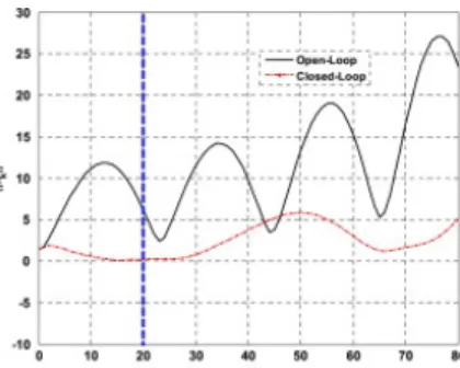
System (33) is simulated with the perturbed controller applied during the first 𝑁𝑁= 20 time steps then removed. Fig. 1 shows the norm of the state of the system with respect to time in both the closed-loop and open-loop cases. The norm of the state remains within the prescribed bound 𝛽𝛽= 11 for every time step over the interval during which the controller is applied, despite the perturbations in its gain. Thus, the controller

developed is performing as expected during the finite-time interval, and the system returns to its controller-free dynamics afterwards.

Fig. 1. Evolution of ‖xk‖ over time for the open-loop and closed-loop cases. The vertical dashed line indicates where the controller is removed.

5.2. Controller gain perturbation magnitude analysis

In this section, the maximum allowable perturbation in the gain of the controller developed as a function of the position of the perturbation vector in a 3D space is examined. Condition (26) on the controller gain perturbation vector implies that ‖𝐾𝐾𝛥𝛥‖ must be less than or equal to 𝜎𝜎𝐾𝐾 in the case of a 3D system with a single input.

Therefore, in a 3D space, the solution for 𝜎𝜎𝐾𝐾 obtained earlier would be the minimum norm of the perturbation

vector for every direction of 𝐾𝐾𝛥𝛥. However, this also means that, in certain directions, ‖𝐾𝐾𝛥𝛥‖ may have a maximum

value, which implies a possibility of a higher upper bound on the allowable perturbations in the controller gain. In order to determine ‖𝐾𝐾𝛥𝛥‖ as a function of its direction, 𝐾𝐾𝛥𝛥 is expressed in spherical coordinates as shown

below.

(34)

𝐾𝐾

_𝛥𝛥

=

𝐾𝐾

̄_𝛥𝛥

[

𝑠𝑠𝑖𝑖𝑛𝑛𝑠𝑠𝑠𝑠𝑠𝑠𝑠𝑠𝑠𝑠 𝑠𝑠𝑖𝑖𝑛𝑛𝑠𝑠𝑠𝑠𝑖𝑖𝑛𝑛𝑠𝑠 𝑠𝑠𝑠𝑠𝑠𝑠𝑠𝑠

]

where 𝐾𝐾̄𝛥𝛥=‖𝐾𝐾𝛥𝛥‖,−90°≤ 𝑠𝑠 ≤+90°, and −180°≤ 𝑠𝑠 ≤+180°.

Moreover, conditions (7), (8), (9) are feasible for the solution of the unknown variables, 𝑄𝑄1,𝑄𝑄2,𝑌𝑌=

𝑌𝑌𝑟𝑟,𝑏𝑏1,𝛿𝛿,𝛼𝛼1,𝛼𝛼2, and 𝛼𝛼3 obtained from (27), (8), (9) with the value of 𝐾𝐾𝑟𝑟 assigned to 𝐾𝐾 and, consequently, the

value of 𝑌𝑌𝑟𝑟 assigned to 𝑌𝑌. With all the variables in (7) known, the controller gain is perturbed by adding 𝐾𝐾𝛥𝛥 to it.

For a fixed direction of 𝐾𝐾𝛥𝛥 (i.e. one set of values of 𝑠𝑠 and 𝑠𝑠), 𝐾𝐾

̄

𝛥𝛥 is incrementally increased until (7) is no longer

feasible. Then, the values of 𝑠𝑠 and 𝑠𝑠 are varied, and the previous steps are repeated until the ranges of 𝑠𝑠 and 𝑠𝑠 are covered.

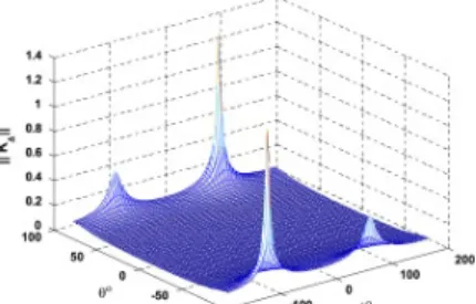
The result obtained is shown in Fig. 2. The minimum value of 𝐾𝐾̄𝛥𝛥 is 0.022, which corresponds to a 4.55%

difference from the value obtained for 𝜎𝜎𝐾𝐾 using the inequalities developed in Theorem 2.

Furthermore, Fig. 2 shows that, for example in the direction of 𝑠𝑠= 75° and 𝑠𝑠= 87°, the controller gain can be perturbed up to 1.305. Even though this result may reflect conservativeness in the results given in Theorem 2, it still shows that the controller design obtained is resilient against perturbations, whose upper bound is at least given by 𝜎𝜎𝐾𝐾.

Fig. 2. Norm of the controller gain perturbation vector 𝐾𝐾𝛥𝛥 as a function of its position in 3D space.

6. Conclusion

A robust and resilient FTB controller design is developed for a class of nonlinear systems with conic-type nonlinearities of uncertain center, known waveform type disturbances, and additive gain perturbations. A solution for the controller gain and the bound on the maximum allowable gain perturbation is obtained using LMI techniques. It is worth noting that the conditions arrived at in this paper reduce to the conditions existing in the literature on the finite-time bounded control of discrete-time linear systems. This fact can be shown by setting the right-hand side term of the conic sector condition and the bounds on the perturbations to zero. Thus, the class of nonlinear systems considered here and the associated results serve as a generalization of previous results. This is due to the fact that this class of systems, in addition to representing several nonlinearities that arise in the control literature, represents simple discrete-time linear systems considered by others in previous works.

References

Amato and Ariola, 2005 F. Amato, M. Ariola Finite-time control of discrete-time linear systems IEEE Transactions of Automatic Control, 50 (5) (2005), pp. 724-729

Amato et al., 2010a F. Amato, M. Ariola, C. Cosentino Finite-time stability of linear time-varying systems: analysis and controller design IEEE Transactions on Automatic Control, 55 (4) (2010), pp. 1003-1008

Amato et al., 2010b F. Amato, M. Ariola, C. Cosentino Finite-time control of discrete-time linear systems: analysis and design Automatica, 46 (5) (2010), pp. 919-924

Amato et al., 2004 Amato, F., Carbone, M., Ariola, M., & Cosentino, C. (2004). Finite-time stability of discrete-time systems. In Proceedings of American control conference, vol. 2 (pp. 1440–1444). Boston,

Massachusetts.

Amato, Cosentino et al., 2010 F. Amato, C. Cosentino, A. Merola Sufficient conditions for finite-time stability and stabilization of nonlinear quadratic systems IEEE Transactions on Automatic Control, 55 (2) (2010), pp. 430-434

Azemi and Yaz, 2001 Azemi, A., & Yaz, E.E. (2001). Full and reduced-order-robust adaptive observers for chaotic synchronization. In Proceedings of American control conference, vol. 3(pp. 1985–1990). Arlington, Virginia.

Chua et al., 1993 L. Chua, C. Wu, A. Hung, G. Zhong A universal circuit for studying and generating chaos-part I: routes to chaos IEEE Transactions on Circuits and Systems I: Fundamental Theory and

Applications, 40 (10) (1993), pp. 732-744

Dorato et al., 1997 Dorato, P., Abdallah, C.T., & Famularo, D. (1997). Robust finite-time stability design via linear matrix inequalities. In Proceedings of the 36th conference on decision & control (pp. 1305–1306). San Diego, California.

ElBsat and Yaz, 2011 ElBsat, M.N., & Yaz, E.E. (2011). Robust and resilient finite-time control of discrete-time nonlinear systems. In 18th IFAC world congress(pp. 6454–6459). Milan, Italy. Preprint.

Garcia et al., 2009 G. Garcia, S. Tarbouriech, J. Bernussou Finite-time stabilization of linear time-varying continuous systems IEEE Transactions on Automatic Control, 54 (2) (2009), pp. 364-369

Johnson, 1980 C.D. Johnson Disturbance-accommodation control: an overview of the subject Journal of Interdisciplinary Modeling and Simulation, 3 (1) (1980), pp. 1-29

Takabashi et al., 2000 Takabashi, R.H.C., Dutra, D.A., Palhares, R.M., & Peres, P.K.D. (2000). On robust non-fragile static state-feedback controller synthesis. In Proceedings of the conference on decision and control (pp. 4909–4914). Sydney, Australia.

Yang et al., 2009 Y. Yang, J. Li, G. Chen Finite-time stability and stabilization of nonlinear stochastic hybrid systems Journal of Mathematical Analysis and Applications, 356 (1) (2009), pp. 338-345

Zhang and An, 2008 W. Zhang, X. An Finite-time control of linear stochastic systems International Journal of Innovative Computing, Information and Control, 4 (3) (2008), pp. 687-694

Zhuang and Liu, 2010 Zhuang, J., & Liu, F. (2010). Finite-time stabilization of a class of uncertain nonlinear systems with time-delay, In Proceedings of 7th conference on fuzzy systems and knowledge discovery (pp. 163–167). Yantai, China.

☆_{The material in this paper was partially presented at the 18th IFAC World Congress, August 28–September 2,}

2011, Milano, Italy. This paper was recommended for publication in revised form by Associate Editor Zongli Lin under the direction of Editor André L. Tits.