Abstraction Refinement Guided by a Learnt Probabilistic Model

arXiv:1511.01874v2 [cs.PL] 10 Nov 2015

Abstraction Refinement Guided by

a Learnt Probabilistic Model

Radu Grigore

Hongseok Yang

Abstract

The core challenge in designing an effective static program analysis is to find a good program abstraction – one that retains only details relevant to a given query. In this paper, we present a new approach for automatically finding such an abstraction. Our approach uses a pessimistic strategy, which can optionally use guidance from a probabilistic model. Our approach applies to parametric static analyses implemented in Datalog, and is based on counterexample-guided abstraction refinement. For each untried abstraction, our probabilistic model provides a probability of success, while the size of the abstraction provides an estimate of its cost in terms of analysis time. Combining these two metrics, probability and cost, our refinement algorithm picks an optimal abstraction. Our probabilistic model is a variant of the Erd˝os–R´enyi random graph model, and it is tunable by what we call hyperparameters. We present a method to learn good values for these hyperparameters, by observing past runs of the analysis on an existing codebase. We evaluate our approach on an object sensitive pointer analysis for Java programs, with two client analyses (PolySite and Downcast).

Categories and Subject Descriptors D.2.4 [Software Engineer-ing]: Software/Program Verification

Keywords Datalog, Horn, hypergraph, probability

1.

Introduction

We wish that static program analyses would become better as they see more code. Starting from this motivation, we designed an ab-straction refinement algorithm that incorporates knowledge learnt from observing its own previous runs, on an existing codebase. For a given query about a program, this knowledge guides the algo-rithm towards a good abstraction that retains only the details of the program relevant to the query. Similar guidance also features in existing abstraction refinement algorithms [4,8,20], but is based on nontrivial heuristics that are developed manually by analysis de-signers. These heuristics are often suboptimal and difficult to trans-fer from one analysis to another. Our algorithm has the potential to improve itself by learning from past runs, and it applies to almost any analysis implemented in Datalog.

[Copyright notice will appear here once ’preprint’ option is removed.]

Prior work on abstraction refinement for Datalog [55] implicitly uses an optimistic strategy: the search is geared towards finding an abstraction that would show the current counterexample to be spu-rious. We take the complimentary approach: our search is geared towards finding an abstraction that would show the current coun-terexample to be unavoidable. Furthermore, we bias the search by using a probabilistic model, which is tuned using information from previous runs of the analysis.

In other approaches to program analysis that are based on learn-ing [43,54], the analysis designer must choose appropriate features. A feature is a measurable property of the program, usually a nu-meric one. Choosing features that are effective for program analy-sis is nontrivial, and involves knowledge of both the analyanaly-sis and the probabilistic model. In our approach, the analysis designer does not need to choose appropriate features.

Instead of observing features, our models observe directly the internal representations of analysis runs. Parametric static analy-ses implemented in Datalog consist of universally quantified Horn clauses, and work by instantiating the universal quantification of these clauses, while respecting the constraints on instantiation im-posed by a given parameter setting. These instantiated Horn clauses are typically implications of the form

h←t1, t2, . . . , tn

and can be understood as a directed (hyper) arc from the source vertices t1, . . . , tn to the target vertex h. Thus, the instantiated Horn clauses taken altogether form a hypergraph. This hypergraph changes when we try the analysis again with a different parameter setting. Given a hypergraph obtained under one parameter setting, we build a probabilistic model that predicts how the hypergraph would change if a new and more precise parameter setting were used. In particular, the probabilistic model estimates how likely it is that the new parameter setting will end the refinement process, which happens when the new hypergraph includes evidence that the analysis will never prove a query. Technically, our probabilistic model is a variant of the Erd˝os–R´enyi random graph model [11]: given a template hypergraphG, each of its subhypergraphsH is assigned a probability, which depends on the values of the hyper-parameters. Intuitively, this probability quantifies the chance that H correctly describes the changes inGwhen the analysis is run with the new and more precise parameter settings. The hyperparam-eters quantify how much approximation occurs in each of the quan-tified Horn clauses of the analysis. We provide an efficient method for learning hyperparameters from prior analysis runs. Our method uses certain analytic bounds in order to avoid the combinatorial ex-plosion of a naive learning method based on maximum likelihood; the explosion is caused byHbeing a latent variable, which can be observed only indirectly.

The next parameter setting to try is chosen by our refinement algorithm based on predictions of the probabilistic model but also

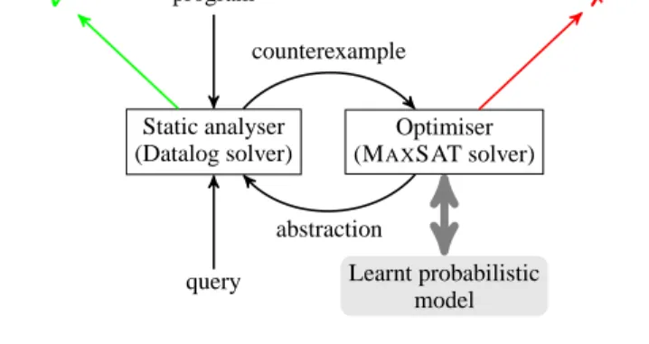
program query ✓ ✗ Static analyser (Datalog solver) Optimiser (MAXSAT solver) Learnt probabilistic model counterexample abstraction Figure 1. Architecture

based on an estimate of the runtime cost. For each parameter set-ting, the probability of successfully handling the query is evaluated by our model, and the runtime is estimated to increase with the precision of the parameter setting. We prove that our method of integrating these two metrics is optimal, under reasonable assump-tions.

The paper starts with an informal overview of our approach (Section 2) and a review of notations from probability theory (Section 3), and is followed by a description of our probabilis-tic model (Section 4) and its learning algorithm (Section 5). The probabilistic model is then used to implement a refinement loop that optimally chooses the next parameter setting (Section 6). The experimental evaluation (Section 7) shows the value of the pes-simistic strategy, but suggests we need better optimisers in order to take full advantage of the probabilistic model.Section 8positions our work in the various attempts to combine probabilistic reasoning and static analyses, andSection 9concludes the paper. Most proofs are in appendices.

2.

Overview

Figure 1gives a high level overview of our abstraction refinement algorithm, and in particular it shows the role of our probabilistic model. The refinement loop is standard, with analysis on one side and refinement on the other. Our contribution lies in the refinement part, which receives guidance from a learnt probabilistic model and chooses the next abstraction by balancing the model’s prediction and the estimated cost of running the analysis under each abstrac-tion.

We assume that the analysis is given and obeys two constraints. The first is that the analysis is implemented in Datalog – it is specified in terms of universally quantified Horn clauses, such as

pointsto(α, ℓ)←precise(α),pointsto(β, ℓ),

assignTo(β, α) (1)

in which all the free variables α, β, ℓ are implicitly universally quantified. We call these clauses Datalog rules. The analysis works by instantiating the quantification of these rules, and thus deriving new facts. A query is a particular fact such as pointsto(x, h), which is an instantiation of the left side of the rule (1), withα:=x and ℓ := h. The query represents an undesirable situation in the program being analysed. The analysis could derive the query because the undesirable situation really occurs at runtime. But, the analysis could also derive the query because it approximates the runtime semantics. Our task is to decide whether it is possible to avoid deriving the query by approximating less. If the query is derived, then the set of all instances of Datalog rules constitute a counterexample, which is then used for refinement.

object x, y, z, v assume x.dirty x.value := 10 0: smudge2(x, y)

0’: y.value := y.value + 2 * x.value 1: smudge3(y, z)

if z.dirty && y.value > 5 v.value := x.value + y.value 2: smudge3(z, v) ... 3: smudge5(x, y) ... 4: smudge7(y, v) assert !v.dirty

Figure 2. Example program to analyse

The second constraint is that the analysis is parametric. For instance, it might have a parameter for each program variable, which specifies whether the variable should be tracked precisely or not. The analysis would encode a setting of these parameters in Datalog by using relations cheap and precise. In fact, the Datalog rule (1) assumes such parametrisation and fires only when the parameter setting dictates the precise tracking of the variableα. For a parametric analysis, an abstraction can be specified by a parameter setting, and so we use these two terms interchangeably.

The refinement part analyses a counterexample, and suggests a new promising parameter setting. If the counterexample derives the query without relying on approximations, then the refinement part reports impossibility and stops [51,55,56]. If the counterexample derives the query by relying on approximations, then the refinement part sets itself the goal to find a similar counterexample that does not rely on approximations. This is a pessimistic goal. To find such a similar counterexample, the analysis must be run with a different parameter setting. Which one? On the one hand, the parameter setting should be likely to uncover a similar counterexample. On the other hand, the parameter should be as cheap as possible. The refinement part uses a MAXSAT solver to balance these desiderata. Consider now the example program inFigure 2. The language is idiosyncratic, and so will be the analysis. The language and the analysis are chosen to allow a concise rendering of the main ideas. In this toy language, each object has two fields, the booleandirty

and the integervalue. Initially, allvaluefields are0. Objectxis dirty at the beginning, and we are interested in whether objectvis dirty at the end. Dirtiness is propagated from one object to another only by the primitive commandssmudgeK. The effect of the com-mandsmudgeK(x, y)is equivalent to the following pseudocode:

if(x.value+y.value) modK= 0

y.dirty:=x.dirty∨y.dirty

That is, if the sum of the values of objectsxandyis a multiple ofK, then dirt propagates fromxtoy.

To decide whether objectvis dirty at the end, an analysis may need to track the values of multiple objects. The values can be changed by guarded assignments. The guard of an assignment can be any boolean expression; the right hand side of an assignment can be any integer expression. In short, tracking values and relations between values could be expensive.

However, tracking all values may also be unnecessary. In the first iteration, the analysis treats all non-smudge commands as

skip. As a result, the analysis knows nothing about the value fields. To remain sound, it assumes that smudge commands always propagate dirtiness; that is, it treats the commandsmudgeK(x, y)

as equivalent to the following pseudocode, dropping the guard: y.dirty:=x.dirty∨y.dirty

x y z v 0 1 2 3 4 1/2 1/3 1/3 1/5 1/7 p ro b ab ili tie s la b el s (p ro g ra m p o in ts )

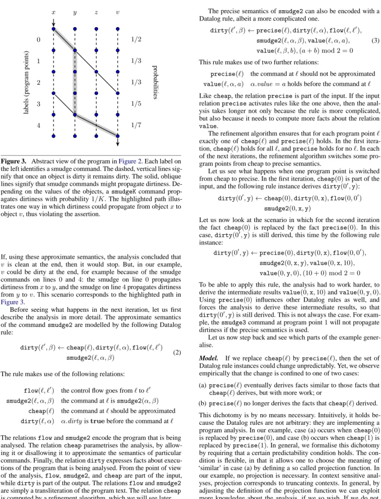
Figure 3. Abstract view of the program inFigure 2. Each label on the left identifies a smudge command. The dashed, vertical lines sig-nify that once an object is dirty it remains dirty. The solid, oblique lines signify that smudge commands might propagate dirtiness. De-pending on the values of the objects, asmudgeKcommand prop-agates dirtiness with probability1/K. The highlighted path illus-trates one way in which dirtiness could propagate from objectxto objectv, thus violating the assertion.

If, using these approximate semantics, the analysis concluded that v is clean at the end, then it would stop. But, in our example, vcould be dirty at the end, for example because of the smudge commands on lines 0 and 4: the smudge on line 0 propagates dirtiness fromxtoy, and the smudge on line4propagates dirtiness fromytov. This scenario corresponds to the highlighted path in Figure 3.

Before seeing what happens in the next iteration, let us first describe the analysis in more detail. The approximate semantics of the commandsmudge2are modelled by the following Datalog rule:

dirty(ℓ′, β)←cheap(ℓ),dirty(ℓ, α),flow(ℓ, ℓ′)

smudge2(ℓ, α, β) (2)

The rule makes use of the following relations:

flow(ℓ, ℓ′) the control flow goes fromℓtoℓ′

smudge2(ℓ, α, β) the command atℓissmudge2(α, β) cheap(ℓ) the command atℓshould be approximated

dirty(ℓ, α) α.dirtyistruebefore the command atℓ

The relationsflowandsmudge2encode the program that is being analysed. The relationcheapparametrises the analysis, by allow-ing it or disallowallow-ing it to approximate the semantics of particular commands. Finally, the relationdirtyexpresses facts about execu-tions of the program that is being analysed. From the point of view of the analysis,flow,smudge2, andcheapare part of the input, whiledirtyis part of the output. The relationsflowandsmudge2

are simply a transliteration of the program text. The relationcheap

is computed by a refinement algorithm, which we will see later.

The precise semantics ofsmudge2can also be encoded with a Datalog rule, albeit a more complicated one.

dirty(ℓ′, β)←precise(ℓ),dirty(ℓ, α),flow(ℓ, ℓ′),

smudge2(ℓ, α, β),value(ℓ, α, a),

value(ℓ, β, b),(a+b) mod 2 = 0

(3)

This rule makes use of two further relations:

precise(ℓ) the command atℓshould not be approximated

value(ℓ, α, a) α.value=aholds before the command atℓ Likecheap, the relationpreciseis part of the input. If the input relationpreciseactivates rules like the one above, then the anal-ysis takes longer not only because the rule is more complicated, but also because it needs to compute more facts about the relation

value.

The refinement algorithm ensures that for each program pointℓ exactly one ofcheap(ℓ)andprecise(ℓ)holds. In the first itera-tion,cheap(ℓ)holds for allℓ, andpreciseholds for noℓ. In each of the next iterations, the refinement algorithm switches some pro-gram points from cheap to precise semantics.

Let us see what happens when one program point is switched from cheap to precise. In the first iteration,cheap(0)is part of the input, and the following rule instance derivesdirty(0′_,y):

dirty(0′,y)←cheap(0),dirty(0,x),flow(0,0′) smudge2(0,x,y)

Let us now look at the scenario in which for the second iteration the fact cheap(0) is replaced by the fact precise(0). In this case,dirty(0′,y)is still derived, this time by the following rule instance:

dirty(0′,y)←precise(0),dirty(0,x),flow(0,0′),

smudge2(0,x,y),value(0,x,10),

value(0,y,0),(10 + 0) mod 2 = 0

To be able to apply this rule, the analysis had to work harder, to derive the intermediate resultsvalue(0,x,10)andvalue(0,y,0). Using precise(0) influences other Datalog rules as well, and forces the analysis to derive these intermediate results, so that

dirty(0′,y)is still derived. This is not always the case. For exam-ple, thesmudge3command at program point1will not propagate dirtiness if the precise semantics is used.

Let us now step back and see which parts of the example gener-alise.

Model. If we replacecheap(ℓ)byprecise(ℓ), then the set of Datalog rule instances could change unpredictably. Yet, we observe empirically that the change is confined to one of two cases: (a)precise(ℓ)eventually derives facts similar to those facts that

cheap(ℓ)derives, but with more work; or

(b)precise(ℓ)no longer derives the facts thatcheap(ℓ)derived. This dichotomy is by no means necessary. Intuitively, it holds be-cause the Datalog rules are not arbitrary: they are implementing a program analysis. In our example, case (a) occurs whencheap(0)

is replaced byprecise(0), and case (b) occurs whencheap(1)is replaced byprecise(1). In general, we formalise this dichotomy by requiring that a certain predictability condition holds. The con-dition is flexible, in that it allows one to choose the meaning of ‘similar’ in case (a) by defining a so called projection function. In our example, no projection is necessary. In context sensitive anal-yses, projection corresponds to truncating contexts. In general, by adjusting the definition of the projection function we can exploit more knowledge about the analysis, if we so wish. If we do not,

then it is always possible to choose a trivial projection for which the meaning of ‘similar’ is ‘exactly the same’.

Provided that the predictability condition holds, which is a for-mal way of saying that the dichotomy between cases (a) and (b) holds, it is natural to define the probabilistic model as a variant of the Erd˝os–R´enyi random graph model. Our sets of Datalog rule in-stances are seen as sets of arcs of a hypergraph. Each arc of the hypergraph is either selected or not, with a certain probability. Be-ing selected corresponds to case (a) – havBe-ing a counterpart in the precise hypergraph; being unselected corresponds to case (b) – not having a counterpart in the precise hypergraph.

For the predictability condition and for the projection function, we drew inspiration from abstract interpretation [10]. Intuitively, our projection functions correspond to concretisation maps, and our predictability condition corresponds to correctness of approxima-tion. However, we did not formalise this intuitive correspondence.

Learning. The model predicts that each rule instance is selected (that is, has a precise counterpart) with some probability. How to pick this probability?Figure 3gives an intuitive representation of a set of instances. In particular, each dashed arc and each solid arc represents some rule instance. We assume that instances rep-resented by dashed arcs are selected with probability1. These are instances of some rule which says that a dirty object remains dirty. We also assume that instances represented by solid arcs are selected with probability1/K. These are instances of rules of the form (2), which describe the semantics ofsmudgeKcommands. These proba-bilities make intuitive sense. In particular, it is reasonable to expect that a number is a multiple ofKwith probability1/K.

But, how can we design an algorithm to find these probabilities, without appealing to intuition and knowledge about arithmetic? The answer is that we run the analysis on many programs, and observe whether rule instances have precise counterparts or not. In our example, if the training sample is large enough, we would observe that instances of the form (2) do indeed have counterparts of the form (3) in about1/Kof cases. In general, it is not possible to observe directly which rules have precise counterparts. It is difficult to decide which rule is a counterpart of which rule. Instead, we make indirect observations based on which similar facts are derived.

Refinement. In terms ofFigure 3, refinement can be understood intuitively as follows. We are interested in whether there is a path from the input on the top left to the output on the bottom right. We know the dashed arcs are really present: they have a precise counterpart with probability1. We do not know if the solid arcs are really present: we see them only because we used a cheap parameter setting, and they have a precise counterpart only with probability1/K. We can find out whether the solid arcs are really present or just an illusion, by running the analysis with a more precise parameter setting. But, we have to pay a price, because more precise parameter settings are also more expensive.

The question is then which of the solid arcs should we enquire about, such that we decide quickly whether there is a path from input to output. There are several possible strategies, in particular there is an optimistic strategy and a pessimistic strategy. The op-timistic strategy hopes that there is no path, so objectvis clean at the end. Accordingly, the optimistic strategy considers asking about those sets of solid arcs that could disconnect the input from the output, if the arcs were not really there. The pessimistic strategy hopes that there is a path, so objectvis dirty at the end. Accord-ingly, the pessimistic strategy considers asking about those sets of solid arcs that could connect the input to the output, if the arcs were really there. The highlighted path inFigure 3corresponds to replac-ingcheap(0)byprecise(0), and alsocheap(4)byprecise(4). Thus, let us denote its set of arcs as04. There are two other paths

that the pessimistic strategy will consider, whose sets of arcs are

012and34. The path04gets a probability1/2×1/7of surviving; the path012gets a probability1/2×1/3×1/3of surviving; the path34gets a probability1/5×1/7of surviving. According to probabilities, the path04has the highest chance of showing that vis dirty at the end.

We designed an algorithm which generalises the pessimistic strategy described above by taking into account unions of paths and also the runtime cost of trying a parameter setting. Our refinement algorithm has to work in a more general setting than suggested by Figure 3. In particular, it must handle hypergraphs, not just graphs.

3.

Preliminaries and Notations

In this section we recall several basic notions from probability theory. At the same time, we introduce the notation used throughout the paper.

A finite probability space is a finite set Ω together with a functionPr : Ω→ Rsuch thatPr(ω) ≥ 0for allω ∈ Ω, and

P

ω∈ΩPr(ω) = 1. An event is a subset ofΩ. The probability of an eventAis Pr(A) := X ω∈A Pr(ω) =X ω∈Ω Pr(ω)[ω∈A]

The notation[Ψ] is the Iverson bracket: ifΨis true it evaluates to1, ifΨis false it evaluates to0. A random variable is a function X_{: Ω→ X. For each valuex ∈ X, the set}X−1_{(x)is an event,}

traditionally denoted by(X_{=x). In particular, we writePr(}X₌ x)for its probability; occasionally, we may writePr(x=X_)for the same probability. A boolean random variable is a function X _{: Ω → {0,1}}. For a random variableXwith X ⊆ R, we define its expectationEXby

EX_:=X

x∈X

xPr(X_{=x) =}X ω∈Ω

Pr(ω)X_(ω) In particular, ifX_{is a boolean random variable, then}

EX= Pr(X= 1)

EventsA1, . . . , Anare said to be independent when

Pr(A1∩. . .∩An) = n

Y

i=1 Pr(Ai)

Note thatnevents could be pairwise independent, but still depen-dent when taken altogether. Random variablesX_{1, . . . ,}X_nare said to be independent when the events(X₁ = x1), . . . ,(X_n = xn) are independent for allx1, . . . , xnin their respective domains. In particular, ifX₁, . . . ,X_n are independent boolean random vari-ables, thenX1_∧. . .∧X_nis also a boolean random variable, and

E(X_1∧. . .∧X_n) =

n

Y

i=1 EX_i

EventsAandBare said to be incompatible when they are disjoint. In that case,Pr(A∪B) = Pr(A) + Pr(B). In particular, if X₁, . . . ,X_n are boolean random variables such that the events

(X₁= 1), . . . ,(X_n= 1)are pairwise incompatible, then

E(X_1∨. . .∨X_n) = n X i=1 EX_i

4.

Probabilistic Model

The probabilistic model predicts what analyses would do if they were run with precise parameter settings. To make such predic-tions, the model relies on several assumptions: the analysis must be implemented in Datalog (Section 4.1) and its precision must be

configurable by parameters (Section 4.2); furthermore, increasing precision should correspond to invalidating some derivation steps (Section 4.3). Given probabilities that individual derivation steps survive the increase in precision, we compute probabilities that sets of derivation steps survive the increase in precision (Section 4.4). Given which set of derivation steps survives the increase in preci-sion, we can tell whether a given query, which signifies a bug, is still reachable (Section 4.5).

4.1 Datalog Programs and Hypergraphs

We shall use a simplified model of Datalog programs, which is essentially a directed hypergraph. The semantics will then be given by reachability in this hypergraph. For readers already familiar with Datalog, it may help to think of vertices as elements of Datalog relations, and to think of arcs as instances of Datalog rules with non-relational constraints removed. For readers not familiar with Datalog, simply thinking in terms of the hypergraph introduced below will be sufficient to understand the rest of the paper.

We assume a finite universe of facts. An arc is a pair(h, B)

of a headhand a bodyB; the head is a fact; the body is a set of facts. A hypergraph is a set of arcs. The vertices of a hypergraph are those facts that appear in its arcs. If a hypergraphGcontains an arc(h, B), then we say thathis reachable fromB inG. In general, given a hypergraphGand a setT of facts, the setRGT of facts reachable fromTinGis defined as the least fixed-point of the following recursive equation:

{h|(h, B)∈GandB⊆ RGT} ∪T ⊆ RGT The following monotonicity properties are easy to check.

Proposition 1. LetG,G1andG2be hypergraphs; letT,T1andT2

be sets of facts.

(a) IfT1⊆T2, thenRGT1⊆ RGT2.

(b) IfG1⊆G2, thenRG1T ⊆ RG2T.

Given a hypergraphGand a setT of facts, the induced

sub-hypergraphG[T]retains those arcs that mention facts fromT: G[T] :={(h, B)∈G|h∈TandB⊆T}

4.2 Analyses

We use Datalog programs to implement static analyses that are parametric and monotone. Thus, the Datalog programs we consider have additional properties:

1. Because the Datalog program implements a static analysis, a subset of facts encode queries, corresponding to assertions in the program being analysed.

2. Because the static analysis is parametric, a subset of facts en-code parameter settings.

3. Because the static analysis is monotone, parameter settings that are more expensive are also more precise.

For example, in Section 2, queries are facts from the relation

dirty; parameter settings are encoded by relations cheap and

precise; and switching a parameter from cheap to precise

makes the analysis more expensive but cannot grow the relation

dirty.

If we only assume that the analysis is parametric, monotone, and implemented in Datalog, then we can already make good pre-dictions in some cases, such as the case of the analysis inSection 2. In other cases, we require more information about the relationship between what the analysis does when run in a precise mode and what the analysis does when run in an imprecise mode. We assume that this information comes in the form of a partial function that projects facts. The technical requirements on the projection func-tion are mild, so the analysis designer has considerable leeway in

choosing an appropriate projection. In some cases, the choice is straightforward. For example, if the analysis isk-object sensitive, meaning that it tracks calling contexts using sequences of alloca-tion sites, then a good choice of projecalloca-tion corresponds to truncat-ing these sequences.

An analysis A is a tuple (G, Q, P, p0, p1, π), where Gis a

hypergraph called the global provenance,Qis a set of facts called

queries,P is a finite set of parameters, the encoding functions p0 and p1 map parameters to facts, andπ is a partial function

from facts to facts called projection. A parameter settingaof an analysisAis an assignment of booleans to the parametersP. We sometimes refer to parameter settings as abstractions, for brevity. We encode the abstractionaas two sets of facts,P0(a)andP1(a), defined by

Pk(a) :={pk(x)|x∈Panda(x) =k} fork∈ {0,1}

The setA(a)of facts derived by the analysisAunder abstractiona is defined to beRG P0(a)∪P1(a). Abstractions form a complete

lattice with respect to the pointwise order:a≤a′_iffa(x)≤a′_(x) for all x ∈ P. We write ⊥for the cheapest abstraction that assigns0to all parameters, and⊤for the most precise abstraction that assigns1to all parameters.

For an analysis A, we sometimes consider the restriction of its hypergraph to those facts derived under a given abstractiona: Ga_{:=G[A(a)]. In particular,G}⊥_{is called the cheap provenance,} andG⊤_{is called the precise provenance.}

An analysis is well formed when it obeys further restrictions: (i) facts derived under the cheapest abstraction are fixed-points of the projection,π(x) = xforx ∈ A(⊥), (ii) the image of the projectionπis included inA(⊥), (iii) only fixed-points project on queries,π−1(q) ⊆ {q}forq ∈ Q, (iv) the encoding functions p0 andp1 are injective and have disjoint images, and (v)

projec-tion is compatible with parameter encoding,π◦p1 = p0. From

(i) and (ii) it follows thatπ is idempotent. These conditions are technical: they ease the treatment that follows, but do not restrict which analyses can be modelled.

An analysisAis said to be monotone when the set of derived queries decreases as a function of the abstraction:a≤a′_implies

Q∩ A(a)

⊇ Q∩ A(a′)

.

We can now formally define the main problem.

Problem 2. Given are a well formed, monotone analysisA, and a queryq forA. Does there exist an abstractionasuch thatq /∈ A(a)?

Because the analysis is monotone,q∈ A(a)for allaif and only ifq∈ A(⊤). Thus, one way to solve the problem is to check ifqis derived byAunder the most precise abstraction⊤. However, this is typically too expensive. Instead, we consider a class of solutions called monotone refinement algorithms. A monotone refinement algorithm evaluates the analysis for a sequencea1 ≤ · · · ≤ an of abstractions. Refinement algorithms terminate when one of two conditions holds: (i)q /∈ A(an)or (ii)q ∈ RGan P₁(a_n)_{. It is} easy to see whyq /∈ A(an) implies thatProblem 2has answer ‘yes’. It is less easy to see why q ∈ RGan P1(a_n) implies thatProblem 2has answer ‘no’. Intuitively, this second termination condition says that the queryqis reachable even if we rely only on precise semantics. In other words, our abstract counterexample does not actually have any abstract step. Formally, we rely on the following lemma:

Lemma 3. Letq be a query for a well formed, monotone analy-sisA. Ifq∈ RGa P1(a)for some abstractiona, thenq∈ A(a′) for all abstractionsa′_.

Proof. ByProposition 1(a),q ∈ RGa P1(a) = R_G P1(a) ⊆

RG P1(⊤)

=A(⊤). We conclude by noting that the analysis is monotone.

4.3 Predictability

The precise provenanceG⊤_{contains all the information necessary} to answerProblem 2. Unfortunately, the precise provenanceG⊤is typically very large and hard to compute. In contrast, the cheap provenance G⊥ is typically smaller and easier to compute. In fact, most refinement algorithms start with the cheapest abstraction, a1=⊥. Fortunately, we observed empirically thatG⊤andG⊥are

compatible, in a way made precise next.

We begin by lifting the projectionπto setsTof facts as follows: π(T) :={t′|t′=π(t)andt∈T}

In particular, if the partial functionπis not defined for anyt∈T, thenπ(T) =∅. Our empirical observation is that

π◦ RG⊤◦P₁=R_H◦π◦P₁ for someH⊆G⊥ (4)

An analysisAthat obeys condition (4) is said to be predictable. A hypergraphHthat witnesses condition (4) is said to be a predictive

provenance of analysisA. For a predictable analysis, reachability and projection almost commute on the image ofP1, except that if

projection is done first, then reachability must ignore some arcs. The inspiration for condition (4) came from the notion of correct approximation, as used in abstract interpretation. But, it is not the same. We tested condition (4) on analyses that do not explicitly follow the abstract interpretation framework, and we were surprised that it holds. Then we designed the example analysis fromSection 2 so that the reason why condition (4) holds is apparent: Datalog rules come in pairs, one encoding precise semantics, the other encoding approximate semantics. But, for real analyses, we could not discern any such simple reason. Thus, we consider our empirical finding as surprising and intriguing.

Recall that refinement algorithms use two termination condi-tions:q /∈ A(a)andq ∈ RGa P1(a). Predictive provenances help us evaluate the termination conditions of refinement algo-rithms.

Lemma 4. LetAbe a well formed, monotone analysis. Letabe an abstraction, and letHbe a predictive provenance. Finally, letq be a query derived byAunder the cheapest abstraction⊥. (a) Ifq /∈ A(a), thenq /∈ RG⊥(P0(a))andq /∈ R_H(π(P1(a))).

(b) Also,q∈ RGa P₁(a)if and only ifq∈ R_H(π(P1(a))). Part (a) lets us approximate the termination condition q /∈ A(a); part (b) lets us evaluate the termination condition q ∈ RGa P1(a). In both cases, only small parts of the global prove-nanceGare used, namelyG⊥andH. The assumptionq ∈ A(⊥)

is reasonable: otherwise the refinement algorithm terminates after the first iteration.

Proof. Assume thatq∈ RH(π(P1(a))). We have

RH(π(P1(a))) =π RG⊤(P1(a)) by (4) q∈π RG⊤(P1(a)) ⇒q∈ RG⊤(P1(a)) byπ−1(q)⊆ {q} RG⊤(P1(a)) =R_Ga(P1(a))⊆ A(a) _byProp.1(a) Putting these together, we conclude thatq ∈ A(a). Using a very similar argument we can show that q ∈ RG⊥(P0(a)) implies

q∈ A(a). This concludes the proof of part (a). The proof of part (b) is similar.

Lemma 4tells us that we could evaluate termination conditions more efficiently if we knew a predictive provenance. Alas, we do not know a predictive provenance.

4.4 Probabilities of Predictive Provenances

If we do not know a predictive provenance, then a naive way for-ward is as follows: enumerate each possible predictive provenance, see what it predicts, and take an average of the predictions. Our model is only marginally more complicated: it considers some pos-sible predictive provenances as more likely than others. On the face of it, enumerating all possible predictive provenances takes us back to an inefficient algorithm. We will see later how to deal with this problem (Section 6). Now, let us define the probabilistic model for-mally.

The blueprint of the probabilistic model is given by a cheap provenanceG⊥. To each arce∈G⊥, we associate a boolean ran-dom variableS_e, and call it the selection variable ofe. Selection variables are independent but may have different expectations. We partitionG⊥_{into typesG}⊥

1, . . . , G⊥t , and we do not require selec-tion variables to have the same expectaselec-tion unless they have the same type. Each typeG⊥k has an associated hyperparameterθk: ife ∈ G⊥k, then we say that e has typek, and we require that

ES_{e =θk}. Recall thatES_{e = Pr(}S_{e = 1)}. We define, in terms of the selection variables, a random variableHwhose values are predictive provenances, by requiring thatS_e= [e∈H]. Thus, the probability of a predictive provenanceHis

Pr(H=H) = t Y k=1 θ|G ⊥ k∩H| k (1−θk)|G ⊥ k\H| ₍₅₎

For example, if all arcs have the same type, then the model has only one hyperparameterθ, andPr(H_=H)isθ|H|_(1−θ)|G⊥\H|_{. At} the other extreme, if all arcs have their own type, then the model has one hyperparameterθefor each arce∈G⊥, andPr(H=H) isQ

e∈G⊥θ

[e∈H]

e (1−θe)[e /∈H].

How many types should there be? Few types could lead to under-fitting, many types could lead to overfitting. In the implementation, we have one type per Datalog rule. Intuitively, this means that we trust the judgement of whoever implemented the analysis.

4.5 Use of the Model

Before using the probabilistic model in a refinement algorithm, we must choose appropriate values for hyperparameters. This is done offline, in a learning phase (Section 5). After learning, each Datalog rule has an associated probability – its hyperparameter.

After the first invocation of the analysis we know the cheap provenanceG⊥_{, which we use as a blueprint for the probabilistic} model. Then, our model predicts whetherq∈ RGa(P1(a)), where ais some abstraction not yet tried. Recall thatq∈ RGa(P1(a))is one of the termination conditions. The hypergraphGa_{is unknown,} and thus we model it by a random variableGa_{. However, we} do know fromLemma 4(b) thatq ∈ RGa(P1(a))_{if and only if} q∈ RH(π(P1(a))). Thus, Pr q∈ RGa(P1(a)) = Pr q∈ R_H(π(P1(a))) = X R q∈R Pr RH(π(P1(a))) =R

whereRranges over subsets of vertices ofG⊥. It remains to com-pute a probability of the formPr RHT = R

. Explicit expres-sions for such probabilities are also needed during learning, so they are discussed later (Section 5).

Intuitively, one could think that the refinement algorithm runs a simulation in which the static analyser is approximated by the probabilistic model. However, it would be inefficient to actually run a simulation, and we will have to use heuristics that have a similar effect (Section 6), namely to minimise the expected total runtime.

5.

Learning

The probabilistic model (Section 4) lets us compute the probability that a given abstraction will provide a definite answer, and thus terminate the refinement. These probabilities are computed as a function of hyperparameters. The values of the hyperparameters, however, remain to be determined. To find good hyperparameters, we shall use a standard method from machine learning, namely MLE (maximum likelihood estimation).

MLE works as follows. First, we set up an experiment. The re-sult of the experiment is that we observe an event O. Next, we compute the likelihoodPr(O)according to the model, which is a function of the hyperparameters. Finally, we pick for hyperparame-ters values that maximise the likelihood.

The standard challenge in deploying the MLE method is in the last phase: the likelihood is typically a complicated function of the hyperparameters. Often, to maximise the likelihood, analytic meth-ods do not exist, and numeric methmeth-ods could be unstable or ineffi-cient. This is indeed the case for our model: analytic methods do not apply, and many numeric methods are inefficient. But, we did find one numeric method that is both stable and efficient (Section 7.2). In addition to the standard challenge, our setting presents an addi-tional difficulty. The expression ofPr(O)is exponentially large if the cheap provenance has cycles. We will handle this difficulty by finding bounds that approximatePr(O).

5.1 Training Experiment

For the training experiment, we collect a set of programs. For the formal development, it is convenient to consider the set of programs as one larger program. We run the analysis on this large training program several times, each time under a different abstraction. The abstractionsa1, . . . , anare chosen randomly, with bias. In partic-ular, they have to be cheap enough so that the analysis terminates in reasonable time. As a result of running the analysis, we observe the provenancesGa1_{, . . . , G}an

. To connect these observed prove-nances to a probabilistic event, we shall use the predictability con-dition (4) together with the following simple fact.

Proposition 5. LetGbe a hypergraph, and letT1andT2be sets of

facts. IfT1⊆T2, thenRGT1=RG′T₁, whereG′=G[R_GT2].

Corollary 6. Leta be an abstraction for analysis A. We have

RG⊤(P1(a)) =R_Ga(P1(a))_.

Given an efficient way to compute the projectionπ, we can compute the sets of factsRk := π RGak(P₁(a_k)), for each k ∈ {1, . . . , n}. UsingCorollary 6and condition (4), we have thatRk = RH(π(P1(ak))), fork ∈ {1, . . . , n}. We define the following events:

Ok := RH(π(P1(a_k))) =R_k fork∈ {1, . . . , n} O := O1∩. . .∩On

The eventO is what we observe. It is completely described by the pairs(ak, Rk). The abstractionakis sampled at random. The setRkof facts is easily computed fromGak. The provenanceGak is obtained from the set of instantiated Datalog rules during the analysis under abstractionak, and it records all the reasoning steps of the analysis.

5.2 Bounds on Likelihood

There appears to be no formula that computes the likelihoodPr(O)

and that is not exponentially large. However, there exist reasonably small formulas that provide lower and upper bounds. We shall use the lower bound for learning, and we shall use both bounds to evaluate the quality of the model.

One could define different bounds on likelihood. Our choice re-lies on the concept of forward arc, which leads to several desirable

properties we will see later. Given a hypergraphG, we define the

distanced(_TG)(h)from verticesTto vertexhby requiringd(_TG)to be the unique fixed-point of the following equations:

d(_TG)(h) = 0 ifh∈T d(_TG)(h) =∞ ifh6∈ RGT d(_TG)(h) = min e=(h,B)∈Gmaxb∈B(d (G) T (b) + 1) otherwise

We omit the superscript when the hypergraph is clear from context. A forward arc with respect toT is an arce = (h, B) ∈Gsuch thatdT(h)> dT(b)for everyb∈B.

Theorem 7. Consider the probabilistic model associated with the

cheap provenance G⊥ _{of some analysis A. Let T}

1, . . . , Tn and R1, . . . , Rn be subsets of vertices ofG⊥. Ifh /∈ B for all arcs

(h, B) inG⊥ _{and R}

k ⊆ RG⊥T_k for allk, then we have the

following lower and upper bounds onPr Tn

k=1(RHT_k=R_k): Y e∈N E ¯S_e Y h Ch6=∅ X E1 E1⊆Ah ∀k∈Ch, E1∩Fk6=∅ Y e∈E1 ES_e Y e∈Ah\E1 E ¯S_e ≤ Pr n \ k=1 RHTk=Rk ≤ Y e∈N E ¯S_e Y h Ch6=∅ X E1 E1⊆Ah ∀k∈Ch, E1∩Dk6=∅ Y e∈E1 ES_e Y e∈Ah\E1 E ¯S_e where

N :={(h′, B′)∈G⊥|B′⊆Rk′andh′∈/R_k′ for somek′}

Ch:={k′|h∈Rk′\T_k′} A_h:={(h, B′)∈G⊥} \N

Dk:={(h′, B′)∈G⊥|B′⊆Rk}

Fk:={e= (h′, B′)∈Dk|eis a forward arc w.r.t.Tk} Intuitively, the arcs inN are those arcs that were observed to be not selected; thus, the factorQ

e∈NE ¯Se. For each reachable vertex, there is a factor that requires a justification, in terms of other reachable vertices and in terms of selected arcs. Let us consider a simple example, in which the lower and upper bounds coincide: there are four arcsek = (h,{bk}) fork ∈ {1,2,3,4}, and we observedR1={b1}, R2={b1, b2, b4, h}, andR3={b3, b4, h}.

InR1, vertexhis not reachable butb1is, soSe1must not hold. In

R2, vertexhis reachable and could be justified by one ofe1, e2, e4,

soS_{e1 ∨}S_e2∨S_e4 must hold. InR3, vertexhis reachable and

could be justified by one ofe3, e4, soSe3∨Se4must hold. In all,

¯

S_e1∧(S_e1∨S_e2∨S_e4)∧(S_e3∨S_e4)

= ¯S_e1∧(S_e2∨S_e4)∧(S_e3∨S_e4) (6)

must hold. The expectation of this quantity is written inTheorem 7 asE ¯S_e1(E ¯Se2E ¯Se3ESe4 +· · ·+ ESe2ESe3ESe4), where

the inner sum enumerates the models of(S_e2∧S_e3)∨S_e4. The situation becomes more complicated when the hypergraph has cycles. In the presence of cycles, the recipe from the previ-ous example does not compute the likelihood, but it does compute an upper bound. The reason is that it counts all cyclic justifica-tions as if they were valid. Indeed, this is the upper bound given inTheorem 7. For the lower bound, we first eliminate cycles by dropping some arcs, thus lowering the likelihood; then, we apply the same recipe.Theorem 7indicates that the arcs which should be dropped are the nonforward arcs. Why is this a good choice? One might think that we should drop a minimum number of arcs if we want a good lower bound. However, (1) it is NP-hard to find the

minimum number of arcs [26, Feedback Arc Set], and (2) the set of such arcs is not uniquely determined. In contrast, we can find the set of nonforward arcs in polynomial time, and the solution is unique.

Another nice property of the set of forward arcs is that, if for each reachable vertex h we retain at least one forward arc whose head ish, then all reachable vertices remain reachable. This property is desirable for detecting impossibility (seeLemma 15). In terms of the lower bound, this property means that we never lower bound a positive probability by0.

In the implementation, we sometimes heuristically drop forward arcs, in order to keep the size of the formula small. But, we only choose to drop a forward arc with headhif there are more than

8forward arcs with headh. For example, if we drop arce2in our

running example, the effect is that we lower bound (6) by

¯

S_e1∧S_e4∧(S_e3∨S_e4)

We simply drop the corresponding variableS_e2 from the formula, thus making the formula smaller. Similarly, we can reduce the size of the formula for the upper bound, at the cost of weakening the bond. This time, we drop clauses rather than variables. For example, we can upper bound (6) by

¯

S_e1∧(S_e2∨S_e4)

For each vertex, our implementation drops all clauses except for the longest one.

Although the probabilistic model is simple, computing the like-lihood of an event of the form ‘RHT₁=R₁and. . .andRHT_n= Rn’ is not computationally easy.Appendix Agives an exact for-mula that has size exponential in the number of vertices of the cheap provenance, but also points to evidence that a significantly smaller formula is unlikely to exist. The size explosion is caused mainly by the cycles of the cheap provenance. Theorem 7gives likelihood lower and upper bounds that are exponential only in the maximum in-degree of the cheap provenance. These formulas are still too large to be used in practice. However, there are simple heuristics that can be applied to reduce the size of the formulas, at the cost of weakening the bounds.

We use the lower bound to learn hyperparameters (Section 7.2). We use the upper bound to measure the quality of the learnt hyper-parameters (Section 7.3).

5.3 Results

We learnt hyperparameters for a flow insensitive but object sen-sitive aliasing analysis. The aliasing analysis is implemented in

59Datalog rules. All but5rules get a hyperparameter of1. A rule with a hyperparameter of 1is a rule that was not observed to be involved in any approximation, in the training set. For two of the re-maining five rules, the learnt hyperparameters were essentially ran-dom, because the likelihood lower bound did not depend on them. The reason is that the training set did not contain enough data, or that the lower bound was too weak.

For the remaining three rules the hyperparameters were0.997,

0.985, and0.969. These values were robust, in the sense that they varied little when the training subset changed. For example, the rule with a hyperparameter of0.969is

CVC(c, u, o)←DVDV(c, u, d, v),CVC(d, v, o),VCfilter(u, o)

Looking briefly at the aliasing analysis implementation we see that (a)CVC(c, u, o)means ‘in contextc, variableumay point to ob-jecto’, and (b) the relationDVDVis responsible for copying method arguments and returned values. We interpret this as evidence that the approximations done by the aliasing analysis are closely related to approximations of the call graph.

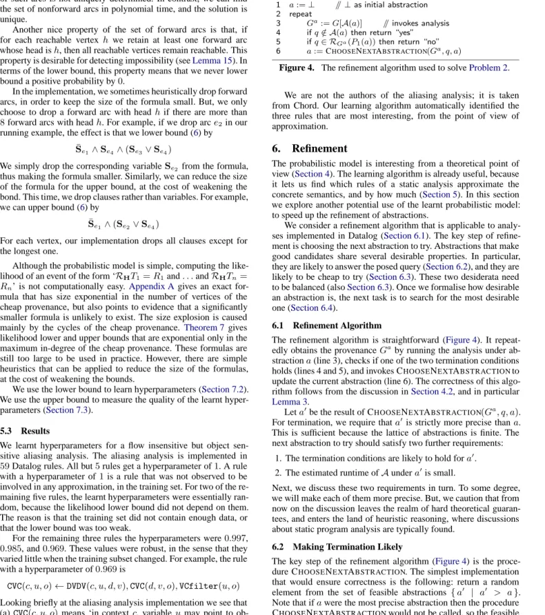
Given: A well formed, monotone analysisA, and a queryq.

SOLVE

1 a:=⊥ //⊥as initial abstraction

2 repeat

3 Ga_:=G[A_{(a)] // invokes analysis}

4 ifq /∈ A_{(a)then return “yes”}

5 ifq∈ R_Ga(P1(a))then return “no”

6 a:=CHOOSENEXTABSTRACTION(Ga, q, a)

Figure 4. The refinement algorithm used to solveProblem 2. We are not the authors of the aliasing analysis; it is taken from Chord. Our learning algorithm automatically identified the three rules that are most interesting, from the point of view of approximation.

6.

Refinement

The probabilistic model is interesting from a theoretical point of view (Section 4). The learning algorithm is already useful, because it lets us find which rules of a static analysis approximate the concrete semantics, and by how much (Section 5). In this section we explore another potential use of the learnt probabilistic model: to speed up the refinement of abstractions.

We consider a refinement algorithm that is applicable to analy-ses implemented in Datalog (Section 6.1). The key step of refine-ment is choosing the next abstraction to try. Abstractions that make good candidates share several desirable properties. In particular, they are likely to answer the posed query (Section 6.2), and they are likely to be cheap to try (Section 6.3). These two desiderata need to be balanced (alsoSection 6.3). Once we formalise how desirable an abstraction is, the next task is to search for the most desirable one (Section 6.4).

6.1 Refinement Algorithm

The refinement algorithm is straightforward (Figure 4). It repeat-edly obtains the provenanceGaby running the analysis under ab-stractiona(line 3), checks if one of the two termination conditions holds (lines 4 and 5), and invokes CHOOSENEXTABSTRACTIONto update the current abstraction (line 6). The correctness of this algo-rithm follows from the discussion inSection 4.2, and in particular Lemma 3.

Leta′_{be the result of CHOOSENEXTABSTRACTION(G}a_{, q, a).} For termination, we require thata′_{is strictly more precise thana.} This is sufficient because the lattice of abstractions is finite. The next abstraction to try should satisfy two further requirements:

1. The termination conditions are likely to hold fora′_. 2. The estimated runtime ofAundera′_{is small.}

Next, we discuss these two requirements in turn. To some degree, we will make each of them more precise. But, we caution that from now on the discussion leaves the realm of hard theoretical guaran-tees, and enters the land of heuristic reasoning, where discussions about static program analysis are typically found.

6.2 Making Termination Likely

The key step of the refinement algorithm (Figure 4) is the proce-dure CHOOSENEXTABSTRACTION. The simplest implementation that would ensure correctness is the following: return a random element from the set of feasible abstractions {a′ | a′ > a}. Note that ifawere the most precise abstraction then the procedure CHOOSENEXTABSTRACTIONwould not be called, so the feasible set from above is indeed guaranteed to be nonempty.

One idea to speed up refinement is to restrict the set of feasible solutions to those abstractions that are likely to provide a definite answer. LetAy andAn be the sets of abstractions that will lead

the refinement algorithm to terminate on the next iteration with the answer ‘yes’ or, respectively, ‘no’:

Ay := {a′|a′> aandq /∈ A(a′)}

An := {a′|a′> aandq∈ R_Ga′(P1(a′))}

Of course, exactly one of the two setsAyandAnis nonempty, but

we do not know which. More generally, we cannot evaluate these sets exactly without running the analysis. But, we can approximate them, because CHOOSENEXTABSTRACTIONhas access toGa. For Aywe can compute an upper boundA⊇y; forAnwe use a heuristic

approximationA≈n.

A⊇y := {a′|a′> aandq /∈ RGa(P0(a′))} A≈n := {a′|a′> aandq∈ RH(T(a, a′))} for someH⊆Ga_{, where}

T(a, a′) := P1(a)∪π(P1(a′)\P1(a))

It is easy to see whyA⊇y ⊇Ay; it is less easy to see whyA≈n ≈An.

Let us start with the easy part.

Lemma 8. LetA⊇

y andAybe defined as above. ThenA⊇y ⊇Ay.

Proof. Assume thata′ > a, as in the definitions ofA⊇y and Ay.

ThenP0(a′)⊆P0(a). ByProposition 5andProposition 1, RGa(P0(a′)) =R_G(P₀(a′)) =R

Ga′(P0(a′))⊆ A(a′)

The claimed inclusion now follows.

Let us now discuss the less obvious claim thatA≈

n ≈An. One

could wonder why we did not defineA≈

n by

{a′|a′> aandq∈ RH(π(P1(a′)))}

for some H ⊆ G⊥. This definition is simpler and is also guar-anteed to be equivalent toAn, by the predictability condition (4).

In the implementation, we use the more complicated definition of A≈

n for two reasons. First, we note that (4) impliesA≈n = Anif

a=⊥. Thus, the claim thatA≈

n =Ancan be seen as a

generali-sation of (4). We did not use this generaligenerali-sation of (4) in the more theoretical parts (Section 4andSection 5) because it would com-plicate the presentation considerably. For example, instead of one projectionπ, we would have a family of projections that compose. In principle, however, it would be possible to takeA≈n = Anas

an axiom, from the point of view of the theoretical development. Second, the more complicated definition ofA≈n exploits all the

in-formation available inGa. The simpler version can also incorporate information fromGaby conditioningHto be compatible withGa, via (4). However, this conditioning would only use the projected set of vertices ofGa, rather than its full structure.

Furthermore, the definition ofA≈n used in the implementation

has the following intuitive explanation. The conditionA≈n ≈An

tells us that in order to predict R_Ga′(P₁(a′)) by using Ga we

should do the following: (i) splitP1(a′_)intoP

1(a)andP1(a′)\

P1(a); (ii) use the facts P1(a) as they are, because they already appear inGa_{; (iii) approximate the facts inP}

1(a′)\P1(a)by their

projections, because they do not appear inGa_{; and (iv) define the} predictive provenanceHwith respect toGa_{, because it is the most} precise provenance available so far.

We defined two possible restrictions of the feasible set, namely A⊇y and A≈n. The remaining question is now which one should

we use, or whether we should use some combination of them such as A⊇

y ∩A≈n. The restriction to A⊇y could be called the

optimistic strategy, because it hopes the answer will be ‘yes’; the restriction toA≈

n could be called the pessimistic strategy, because

it hopes the answer will be ‘no’. The optimistic strategy has been

used in previous work [55]. The pessimistic strategy is used in our implementation. We found that it leads to smaller runtime (Section 7.4). It would be interesting to explore combinations of the two strategies, as future work.

In the optimistic strategy, one needs to check whetherA⊇

y =∅.

In this case, it must be thatAy=∅and thus the answer is ‘no’. In

other words, the main loop of the refinement algorithm needs to be slightly modified to ensure correctness. In the pessimistic strategy, it is never the case thatA≈

n = ∅, and so the main loop of the

re-finement algorithm is correct as given inFigure 4. The pessimistic restrictionA≈

n is nonempty because it always contains⊤, by

choos-ingH=Ga_{(seeLemma 15).}

The setA≈n is defined in terms of an unknown predictive

prove-nanceH. Thus, we work in fact with the random variable A≈_n :={a′|a′> aandq∈ RH(T(a, a′))}

defined in a probabilistic model with respect toGa_{, instead ofG}⊥_. We wish to choose an abstractiona′that is likely inA≈_n. In other words, we want to maximisePr(a′ ∈ A≈_{n). There is no simple} expression to compute this probability. For optimisation, we will use the following lower bound.

Lemma 9. LetA≈_{n be defined as above, with respect to an} anal-ysisA, an abstractiona, and a queryq. Leta′be some abstrac-tion such thata′ > a. LetH be some subgraph ofGasuch that q∈ RH(T(a, a′)). Then

Pr(a′∈A≈_{n) ≥} Y e∈H

ES_e whereS_{eis the selection variable of arce.}

Before describing the search procedure (Section 6.4), we must see how to balance maximising the probability of termination with minimising the running cost.

6.3 Balancing Probabilities and Costs

We are looking for an abstraction that is likely to answer the query but, at the same time, is not too expensive. Most of the time, these two desiderata point in opposite directions: expensive abstractions are more likely to provide an answer. This raises the question of how to balance the two desiderata. We model the problem as follows.

Definition 10 (Action Scheduling Problem). Suppose that we have

a list ofm ≥ 1actions, which can succeed or fail. The success probabilities of these actions arep1, . . . , pm∈(0,1], and the costs for executing these actions arec1, . . . , cm>0. Find a permutation σon{1, . . . , m}that minimises the costC(σ):

C(σ) = m X k=1 qk(σ)cσ(k), qk(σ) = k−1 Y j=1 1−pσ(j).

Intuitively,C(σ) represents the average cost of running actions according toσuntil we hit success.

In the setting of our algorithm, themactions correspond to all the possible next abstractionsa′1, . . . , a′m. ThepiisPr(a′i∈A≈n),

and ci is the cost of running the analysis under abstraction a′i. Hence, a solution to this action scheduling problem tells us how we should combine probability and cost, and select the next abstrac-tiona′.

Lemma 11. Consider an instance of the action scheduling problem

(Definition 10). Assume the success probabilities of the actions are independent. A permutationσhas minimum costC(σ)if and only ifpσ(1)/cσ(1)≥ · · · ≥pσ(m)/cσ(m).

Corollary 12. Under the conditions ofLemma 11, if the cost of permutationσis minimum, thenσ(1)∈arg max_ipi/ci.

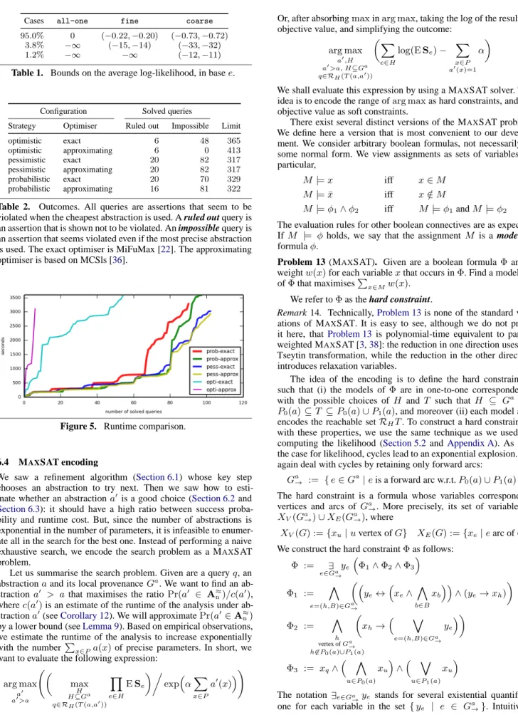
Cases all-one fine coarse 95.0% 0 (−_0.22,−_{0.20) (}−_0.73,−_0.72)

3.8% −∞ ₍−_15,−_{14) (}−_33,−₃₂₎

1.2% −∞ −∞ ₍−_12,−₁₁₎ Table 1. Bounds on the average log-likelihood, in basee.

Configuration Solved queries

Strategy Optimiser Ruled out Impossible Limit

optimistic exact 6 48 365 optimistic approximating 6 0 413 pessimistic exact 20 82 317 pessimistic approximating 20 82 317 probabilistic exact 20 70 329 probabilistic approximating 16 81 322

Table 2. Outcomes. All queries are assertions that seem to be violated when the cheapest abstraction is used. A ruled out query is an assertion that is shown not to be violated. An impossible query is an assertion that seems violated even if the most precise abstraction is used. The exact optimiser is MiFuMax [22]. The approximating optimiser is based on MCSls [36].

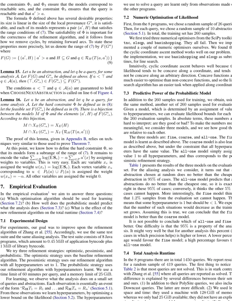
Figure 5. Runtime comparison.

6.4 MAXSAT encoding

We saw a refinement algorithm (Section 6.1) whose key step chooses an abstraction to try next. Then we saw how to esti-mate whether an abstractiona′ is a good choice (Section 6.2and Section 6.3): it should have a high ratio between success proba-bility and runtime cost. But, since the number of abstractions is exponential in the number of parameters, it is infeasible to enumer-ate all in the search for the best one. Instead of performing a naive exhaustive search, we encode the search problem as a MAXSAT problem.

Let us summarise the search problem. Given are a queryq, an abstractionaand its local provenanceGa_{. We want to find an} ab-stractiona′ _{> a that maximises the ratioPr(a}′ _{∈ A}≈

n)/c(a′),

wherec(a′_{)is an estimate of the runtime of the analysis under} ab-stractiona′(seeCorollary 12). We will approximatePr(a′∈A≈_n)

by a lower bound (seeLemma 9). Based on empirical observations, we estimate the runtime of the analysis to increase exponentially with the numberP

x∈Pa(x)of precise parameters. In short, we want to evaluate the following expression:

arg max a′ a′ >a max H H⊆Ga q∈RH(T(a,a′)) Y e∈H ES_e expαX x∈P a′(x) !

Or, after absorbingmaxinarg max, taking the log of the resulting objective value, and simplifying the outcome:

arg max a′ ,H a′>a, H⊆Ga q∈RH(T(a,a′)) X e∈H log(ES_e)− X x∈P a′ (x)=1 α (7)

We shall evaluate this expression by using a MAXSAT solver. The idea is to encode the range ofarg maxas hard constraints, and the objective value as soft constraints.

There exist several distinct versions of the MAXSAT problem. We define here a version that is most convenient to our develop-ment. We consider arbitrary boolean formulas, not necessarily in some normal form. We view assignments as sets of variables; in particular,

M |=x iff x∈M

M |= ¯x iff x /∈M

M |=φ1∧φ2 iff M |=φ1andM |=φ2

The evaluation rules for other boolean connectives are as expected. IfM |= φ holds, we say that the assignmentM is a model of formulaφ.

Problem 13 (MAXSAT). Given are a boolean formulaΦand a weightw(x)for each variablexthat occurs inΦ. Find a modelM ofΦthat maximisesP

x∈Mw(x). We refer toΦas the hard constraint.

Remark 14. Technically,Problem 13is none of the standard vari-ations of MAXSAT. It is easy to see, although we do not prove it here, thatProblem 13 is polynomial-time equivalent to partial weighted MAXSAT [3,38]: the reduction in one direction uses the Tseytin transformation, while the reduction in the other direction introduces relaxation variables.

The idea of the encoding is to define the hard constraint Φ

such that (i) the models ofΦare in one-to-one correspondence with the possible choices ofH and T such that H ⊆ Ga _and P0(a)⊆T ⊆P0(a)∪P1(a), and moreover (ii) each model also encodes the reachable setRHT. To construct a hard constraintΦ with these properties, we use the same technique as we used for computing the likelihood (Section 5.2andAppendix A). As was the case for likelihood, cycles lead to an exponential explosion. We again deal with cycles by retaining only forward arcs:

Ga→ := {e∈Ga|eis a forward arc w.r.t.P0(a)∪P1(a)} The hard constraint is a formula whose variables correspond to vertices and arcs of Ga→. More precisely, its set of variables is XV(Ga→)∪XE(Ga→), where

XV(G) :={xu|uvertex ofG} XE(G) :={xe|earc ofG} We construct the hard constraintΦas follows:

Φ := ∃ e∈Ga → ye Φ1∧Φ2∧Φ3 Φ1 := ^ e=(h,B)∈Ga → ye↔ xe∧ ^ b∈B xb ∧(ye→xh) Φ2 := ^ h vertex ofGa→ h6∈P0(a)∪P1(a) xh→ _ e=(h,B)∈Ga → ye Φ3 := xq∧ ^ u∈P0(a) xu ∧ _ u∈P1(a) xu (8)

The notation ∃e∈Ga

→ye stands for several existential quantifiers,

the constraintsΦ1 and Φ2 ensure that the models correspond to reachable sets, and the constraint Φ3 ensures that the query is reachable and thata′> a.

The formulaΦdefined above has several desirable properties: its size is linear in the size of the local provenanceGa, it is satisfi-able, and each of its models represents a pair(a′, H)that satisfies the range conditions of (7). The satisfiability ofΦis important for the correctness of the refinement algorithm, and it follows from how we remove cycles, by retaining forward arcs. To state these properties more precisely, let us denote the range of (7) byF(Ga₎ where

F(G) :={(a′, H)|a′> aandH ⊆Gandq∈ RH(T(a, a′))} (9)

Lemma 15. Letabe an abstraction, and letqbe a query, for some analysisA. LetF(G)andGa

→be defined as above. Ifa <⊤and q∈ A(a), then(⊤, Ga

→)∈F(Ga→)⊆F(Ga).

The conditionsa < ⊤andq ∈ A(a)are guaranteed to hold when CHOOSENEXTABSTRACTIONis called on line 6 ofFigure 4.

Lemma 16. Let a be an abstraction, and letq be a query, for some analysisA. Let the hard constraint Φbe defined as in (8): let the feasible setF(Ga→)be defined as in (9). There is a bijection between the modelsM ofΦand the elements(a′, H)ofF(Ga→). According to this bijection,

M∩XE(Ga→) =XE(H)

M∩XV(Ga→) =XV RH(T(a, a′))

The proof of this lemma, given inAppendix B, relies on tech-niques very similar to those used to proveTheorem 7.

At this point, we know how to define the hard constraintΦ, so that its models form a subrange of the range of (7). It remains to encode the valueP

e∈Hlog(ESe)−α

P

x∈Pa

′_{(x)by assigning} weights to variables. This is very easy. Each arc variable xe is assigned the weightw(xe) = log(ESe). Each vertex variablexu corresponding to u ∈ P0(a) ∪ P1(a) is assigned the weight

w(xu) =−α. All other variables are assigned the weight0.

7.

Empirical Evaluation

In the empirical evaluation1 we aim to answer three questions: (a) Which optimisation algorithm should be used for learning (Section 7.2)? (b) How well does the probabilistic model predict what the analysis does (Section 7.3)? (c) What is the effect of the new refinement algorithm on the total runtime (Section 7.4)?

7.1 Experimental Design

For experiments, our goal was to improve upon the refinement algorithm of Zhang et al. [55]. Accordingly, we use the same test suite and the same aliasing analysis. The test suite consists of 8 Java programs, which amount to0.45 MiBof application bytecode plus

1 MiBof library bytecode.

We try three refinement strategies: optimistic, pessimistic, and probabilistic. The optimistic strategy uses the baseline refinement algorithm. The pessimistic strategy uses our refinement algorithm with all hyperparameters set to 1. The probabilistic strategy uses our refinement algorithm with hyperparameters learnt. We use a time limit of60minutes per query, and a memory limit of25 GiB. For learning, we observe what the analysis does on a small set of queries and abstractions. Each observation is essentially an event of the form ‘RHT1=R1and. . .andRHTn=Rn’ (Section 5.1). From these observations we learn hyperparameters, by optimising a lower bound on the likelihood (Section 5.2). The hyperparameters

1_{http://rgrig.appspot.com/static/papers/popl2016experiments.html}

we use to solve a query are learnt only from observations made on the other programs.

7.2 Numeric Optimisation of Likelihood

First, from the8programs, we chose a random sample of26queries. Then, for each query, we chose a random sample of10abstractions (Section 5.1). In total, the training set has260samples.

We first tried three numerical optimisers from the SciPy toolkit [23]:

tnc, slsqp, and basinhopping. They all fail. Then we imple-mented a couple of numeric optimisers ourselves. We found that the cyclic coordinate ascent method works well on our problem. In the implementation, we usebasinhoppingandslsqpas subrou-tines, for line search.

Intuitively, cyclic coordinate ascent behaves well because the likelihood tends to be concave along a coordinate, and tends to not be concave along an arbitrary direction. Concave functions are much easier to optimise than non-concave functions, and so the line search algorithm has an easier task when applied along coordinates.

7.3 Predictive Power of the Probabilistic Model

In addition to the260samples used for training, we obtain, using the same method, another set of260samples used for evaluation. Given a model, which is determined by an assignment of values to hyperparameters, we can evaluate likelihood bounds for each of the260evaluation samples. In absolute terms, these numbers are hard to interpret: are they good or bad? To make the numbers more meaningful, we consider three models, and we see how good they are relative to each other.

The three models are:fine,coarse, andall-one. Thefine

model is learnt as described above. Thecoarsemodel is also learnt as described above, but under the constraint that all hyperparam-eters have the same value. Theall-one model simply assigns value1to all hyperparameters, and thus corresponds to the pes-simistic refinement strategy.

Table 1presents the results of the three models on the evaluation set. For the aliasing analysis we consider, it turns out that an abstraction chosen at random does no better than the cheapest abstraction in95%of cases. Theall-onemodel predicts that all abstractions do no better than the cheapest one, so it is exactly right in these95%of cases; conversely, it thinks the other5%of cases cannot happen. More interestingly, thefinemodel thinks that1.2% samples from the evaluation set cannot happen. This means that some hyperparameter is1but should be<1. We expect that the number of such situations would decrease as the training set grows. Assuming this is true, we can conclude that thefine

model is better than thecoarsemodel.

It is not possible to conclude which of all-oneandfineis better. One difficulty is that the95%is a property of the analy-sis. It might very well be that for another analysis this percent (of cases in which precision helps) is higher or lower. A lower percent-age would favour thefinemodel; a high percentage favours the

all-onemodel.

7.4 Total Analysis Runtime

In the8programs there are in total1450queries. We report results for a random sample of419queries. The first thing to notice in Table 2is that most queries are not solved. This is in stark contrast with Zhang et al. [55] where all queries are reported as solved. The difference is explained by several differences between their setup and ours. (1) In addition to their PolySite queries, we also include Downcast queries. The latter are more difficult. (2) We used less space and time: they used a machine with128 GiB of memory, whereas we only had25 GiBavailable; they did not have an explicit time limit, whereas we used1hour as our time limit. (3) One of our modifications to the code (unfortunate, with hindsight), was that we