International Journal of Computational & Neural Engineering (
IJCNE
)
ISSN 2572-7389
Using Multiple Linear Regression and Artificial Neural Network to Predict Surface Roughness in
Turning Operations
Research Article
Ibrahim A Badi1*, Ali G Shetwan2, Maitig A1
1 Mechanical Engineering Department, Misurata University, Libya. 2 Industrial Engineering Department, Misurata University, Libya.
Introduction
Nowadays, due to the increasing demand of higher efficiency and
quality, surface roughness of a machined part plays an important role in the modern manufacturing process. Machined surface characteristics affect the fatigue strength, corrosion resistance and tribological properties of machined components. The quality of
material is determined by surface finish produced after machining.
Therefore, control of the machined surface is essential to safe turning operations [1]. The quality of finished products is defined by how closely the finished product adheres to certain specifications, including dimensions and the quality of the surface
[2]. Therefore, the most important aspects in manufacturing processes are measuring and characterizing of surface properties.
Surface quality is defined and identified by the combination of surface finish, surface texture, and surface roughness. The surface
roughness is one of the important properties of work piece quality in the turning process. Since the cutting conditions impact the quality of the surfaces, thus a work piece may be scrapped or reworked due to improper surface roughness machined. For this reason, several studies have been carried out to predict the value of roughness.
This study aims to develop two mathematical models to predict the surface roughness and to select the required surface roughness by using the Multi-regression model and ANN.
This paper is structured as follows: First, previous similar research
is reviewed briefly. Then the experimental study is presented followed by modeling of surface roughness. Next, prediction and
results are presented and analyzed. Finally, conclusions are made at the end of the paper.
Literature Review
Asiltürk and Cunkas [1] developed a model based on ANN and multiple regression to predict the surface roughness in AISI 1040 steel. It was found that the proposed models are capable of predicting the surface roughness. It was also found that the ANN model estimates the surface roughness with high accuracy compared to the multiple regression model.
Asiltürk and Neseli [3] developed a model to determine the effect of cutting parameters, namely cutting speed, depth of cut and feed rate on surface roughness during machining of AISI 304
Abstract
Quality of surface roughness has a great impact on machine parts during their useful life. The machining process is more
complex, and therefore, it is very hard to develop a comprehensive model involving all cutting parameters. In this paper, the
surface roughness is measured during turning operation at different cutting parameters such as speed, feed rate, and depth of cut. Two mathematical models are developed to predict the surface roughness and to select the required surface
rough-ness by using the Multi-regression model and Artificial Neural Networks (ANN). To test the developed models, 27 pieces
of steel alloy HRC15 were operated and the roughness of their surfaces measured. The results showed that the ANN model estimates the surface roughness with high accuracy compared to the multiple regression model with the average deviation from the real values of about 1%.
Keywords:Predictive; Turning; Artificial Neural Networks; Surface Roughness and Regression.
*Corresponding Author: Ibrahim A. Badi,
Mechanical Engineering Department, Misurata University, Libya. E-mail: [email protected]
Received: November 10, 2017
Accepted: November 24, 2017
Published: November 28, 2017
Citation: Ibrahim A Badi, Ali G Shetwan, Maitig A. Using Multiple Linear Regression and Artificial Neural Network to Predict Surface Roughness in Turning Operations. Int J Comput
Neural Eng. 2017;4(4):91- 97. doi: http://dx.doi.org/10.19070/2572-7389-1700011
Copyright: Ibrahim A Badi© 2017. This is an open-access article distributed under the terms of the Creative Commons Attribution License, which permits unrestricted use, distribution and reproduction in any medium, provided the original author and source are credited.
austenitic stainless. The conclusion of the study was that the feed rate is the dominant factor affecting the surface roughness, which is minimized when the feed rate and depth of cut are set to the lowest level, while the cutting speed is set to the highest level. The percentages of error fall within 1% between the predicted values
and the experimental values.
Patel et al., [4] developed a mathematical model by using ANN technique to predict surface roughness in CNC milling machine.
Several experiments were carried out by using HSS CNC milling
machine. The input parameters of the ANN are spindle speed, feed rate and depth of cut. The results showed that the prediction
of surface roughness is accurate by 91.94% [4].
Parmar and Makwana [5] developed a model to predict surface
roughness by using artificial neural networks. The aim of the study was to find the best cutting parameters value for a specific cutting
condition in milling operation and achieve minimum surface
roughness. Experimental investigation was conducted using the
end milling of mild steel material up to 30 HRC with carbide tool by varying feed rate, speed and depth of cut. The surface roughness was measured using Mitutoyo Surface Roughness
Tester. The results of the study were as follows: the maximum surface roughness value 0.35μm was obtained at the value of 0.06
mm/rev, 80 m/min and 0.2 mm for feed rate, cutting speed and depth of cut respectively.
Aghdeab et al., [6] developed a model to obtain the optimal parameters of CNC turning process that lead to an optimal surface roughness for machining aluminum alloy ENAC43400. The developed objective model was obtained using the regression method and optimized by the simulated annealing method in order to determine the best set of turning parameter values. It
was found that the surface roughness is about (1.06-1.41μm).
Tsao [7] adopted grey Taguchi method to optimize the milling
parameters of A6061P-T651 aluminum alloy with multiple performance characteristics. The experimental results indicated
that the optimal process parameters in milling aluminum alloy can
be effectively determined; the flank wear was decreased from 0.177 mm to 0.067 mm and the surface roughness was decreased from 0.44 μm to 0.24 μm. This result led to a multiple performance
characteristics improvement in milling qualities through the grey Taguchi method.
Fang et al., [8] conducted a study dealing with the neural network modeling and prediction of surface roughness in machining aluminum alloys using data collected from both force and vibration sensors. Two neural network models, including a
Multi-Layer Perceptron (MLP) model and a Radial Basis Function (RBF)
model, were developed. Each model includes eight inputs and
five outputs. The eight inputs include the cutting speed, the ratio
of the feed rate to the tool-edge radius, cutting forces in three
directions, and cutting vibrations in three directions. The five outputs were the five surface roughness parameters. The results of the study showed that the MLP model provided significantly
higher accuracy of prediction for surface roughness than the RBF model did.
Kumar and Narayana [9] developed a model based on a combination of three soft computing techniques namely Adaptive Neuro Fuzzy Inference System, Neural Networks and regression to predict the surface roughness in turning process. The input variables of the model are the machining variables that have a major impact on the surface roughness in turning process such as spindle speed,
feed rate and depth of cut. On the other side, surface roughness is considered as output. Based on the experimental results of the
study, it was observed that surface roughness value increases as the feed rate and depth of cut increases and as the spindle speed increases the surface roughness value decreases. It was also found that the minimum surface roughness value is observed at spindle speed of 150 rpm, feed rate of 0.05 mm/rev and a depth of cut of 0.2 mm respectively.
Dinesh et al., [10] developed an empirical model using Response
Surface Methodology to predict material removal rate (MRR)
and surface roughness in CNC turning of EN24 Alloy Steel.
The influence of four cutting parameters, cutting speed, feed
rate, depth of cut, and tool nose radius on minuscule surface roughness and MRR were analyzed on the basis of Response Surface Methodology approach. It was found that the surface
roughness is (0.43-1.99 μm). Also, it was found that the minimum
speed of 110m/min produces higher MRR. The depth of cut has
an inverse effect on MRR. The maximum depth of cut of 1.0
mm produces higher MRR. Hence higher MRR was achieved by
combining minimum feed rate and maximum depth of cut.
Experimental Study
This section studys the selection of parameters which affect the surface roughness values, type of work piece material and
experimental plan required to conduct the experiment. In turning, the speed and motion of the cutting tool is specified through
several parameters. These parameters are selected for each operation based upon the work piece material, tool material, tool size, and others. Turning parameters that can affect the process are: spindle speed, feed rate and depth of cut. The parameters to
be considered in the study were identified at three levels for each of these factors, as shown in Table (1).
In order to test the developed models, 27 pieces of alloy steel
HRC15 were operated and the roughness of their surfaces measured by ALPA-SM RT-20. The running of the three test
pieces was based on random cut conditions. The experiments
were carried out using CNC turing machine TLC-20B.
Table 1. Experimental Values at Three Levels.
Parameter Cutting speed(m/min) Feed rate (mm/rev) Depth of cut (mm)
Level 1 200 0.12 0.3
Level 2 310 0.22 0.7
Modeling of Surface Roughness
In this paper, two models are developed based on Multi-regression
model and Artificial Neural Networks to predict surface
roughness. The two models have been solved using Microsoft
excel and Neuro software.
Regression Model
The regression model for multiple regression line is shown in
Equation (1) [11]. 0 1 1 2 2
ˆ
ˆ
ˆ
ˆ
Y
=
β
+
β
X
+
β
X
+
...
+
β
kX
k --- (1) Where: Y: dependent variable; 0 ˆ β : Constant or intercept; ˆ kβ : regression slope of Y on independent variable Xk; Xk : Independent variable.
The regression model is solved by using experimental data,
and then roughness values can be predicted. The accuracy of the results of the multiple linear regression model can then be evaluated using R adjusted Square. Also it can be evaluated using F
test significance. If the value of F is less than or equal to 0.05, this
means that the model is statistically acceptable. In the contrary, if the value is more, then the model is unacceptable.
Artificial Neural Networks Modeling
Neural network is a highly flexible modeling tool with the ability to
learn the mapping between input and output parameters [5]. The
main concept of Artificial neural networks (ANNs) is based on
emulating the biological connections between neurons. ANNs can reproduce some functions of human behavior, which are formed
by a finite number of layers with different computing elements
called neurons. In order to construct a network, the neurons are
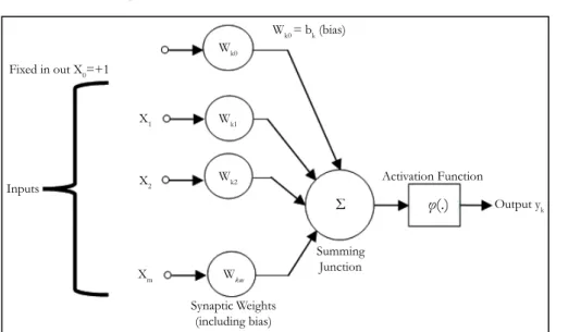
interconnected. As shown in Figure (1), the network consists
of an input layer used to present data, output layer to produce ANN’s response, and one or more hidden layers in between. The organization of connections determines the type and objectives of the ANNs. The processing ability of the network is stored in the inter-unit connection strengths, or weights, which are tuned
in the learning process. The learning algorithm is defined as a
procedure that consists of adjusting the weights and biases of a network that minimizes selected function of the error between the actual and desired outputs [1].
The steps of the learning algorithm of ANN with back-propagation algorithm is as follows [12]:
Step 1: Initialization of the initial weights (w1, w2, w3, ..., wn) = Wn
and Θ represents the threshold.
Step 2: Select learning vector pair (Xn, Yj), where Xn represents input vector.
Xn = (x1, x2, x3, …., xn)
Yj : Represents the required output Yj = (y1, y2, y3, …., yj)
Step 3: Calculating the real output value as follows:
1) Calculate the real output value from the input layer to the
hidden layer. 1 ( ), [ n ] H IH IH i Ii i i Y = f net net =
∑
= X W −θ
--- (2)n: represents the number of elements in the input layer of the network.
2) Calculate the real output value of the hidden layer to the output
layer. 1 ( ), [ p ] O HO HO j Hj j j Y = f net net =
∑
=Y W −θ
---- (3)P: represents the number of elements in the hidden layer of the network.
Figure 1. The Structure of an Artificial Neuron.
Fixed in out X0=+1 Inputs Wk0 Wk1 Wk2 Wkm X1 X2 Xm Synaptic Weights (including bias) Σ Summing Junction φ(.) Activation Function Wk0 = bk (bias) Output yk
Step 4: Calculate the error as follows:
0
j d j
e Y Y
=
−
≠
--- (4)
d: the real value of the roughness.
1) The weights between the output layer and the hidden layer can be modified as follows:
j j j
W
α δ
X
∆
=
and
δ
j=
Y
j(1
−
Y e
j)
j ---(5)2) The weights between the hidden layer and the input layer can be modified as follows: new old i i i
W
=
W
+ ∆
W
i i iW
α
X
δ
∆
=
and i i(1 i) p1 j j j Y Y W δ δ = = −∑
--- (6)Step 5: Repeat the steps from step 2 through step 5 until the desired convergence is obtained, which represents the lowest square rate.
Prediction of Results and Analysis
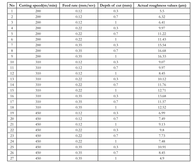
The experiments were conducted for three different levels for each variable, the total number of (27) pieces of alloy HRC15. Table (2) shows the input data for the experiment and the reading
values for surface roughness. The multiple linear regression
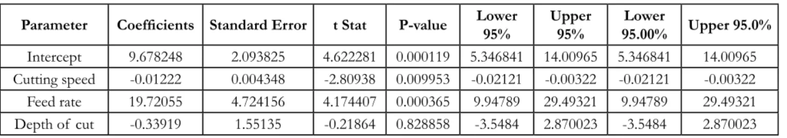
equation constants is obtained by using Excel program. Input experiment data (Speed, Feed rate, and Depth of cut) and the corresponding output data (Experimental roughness data) were entered to the regression model. Table (3) shows results of
multiple linear regression model.
Based on the results of Table (3) the regression equation is given by equation (1).
Y = 9.678248 + (-0.01222 X1) + (19.72055 X2) + (-0.33919X3)(1) Figure (2) shows the real roughness (measured) values and the
roughness obtained from the Multi-regression model for the
number of experiments. It is seen from Figure (2) that there is a
strong relationship between the predictor variables and response variable.
To develop artificial neural networks model, there are many
variables that effect the development of ANN and they must
be identified when creating the network. These variables are as
Table 2. Parameters value and roughness reading for the machined parts.
No Cutting speed(m/min) Feed rate (mm/rev) Depth of cut (mm) Actual roughness values (µm)
1 200 0.12 0.3 5.5 2 200 0.12 0.7 6.32 3 200 0.12 1 6.41 4 200 0.22 0.3 9.97 5 200 0.22 0.7 11.22 6 200 0.22 1 11.43 7 200 0.35 0.3 15.54 8 200 0.35 0.7 16.68 9 200 0.35 1 16.33 10 310 0.12 0.3 9.07 11 310 0.12 0.7 9.97 12 310 0.12 1 8.45 13 310 0.22 0.3 10.12 14 310 0.22 0.7 11.76 15 310 0.22 1 12.71 16 310 0.35 0.3 13.68 17 310 0.35 0.7 11.57 18 310 0.35 1 12.52 19 450 0.12 0.3 6.99 20 450 0.12 0.7 7.49 21 450 0.12 1 9.13 22 450 0.22 0.3 9.8 23 450 0.22 0.7 7.73 24 450 0.22 1 7.48 25 450 0.35 0.3 10.91 26 450 0.35 0.7 8.45 27 450 0.35 1 4.9
follows:
1) Epoch: variable is used to stop learning, where the network
stops learning if the number of iterations reach to the number of
iterations specified.
2) Learning Rate (tr): learning rate and determines the speed of
change of inclination and bias.
The bias can be considered as one of the weights of W0 and its
input (X0 = 1).
3) Initial Weight: The primary weight in the training process.
The previous variables were determined when the network
was created. Thus, 27 networks were created for each network
containing different variables from the other network. For the
Table 3. Results of multiple linearregression model.
Parameter Coefficients Standard Error t Stat P-value Lower95% Upper95% 95.00% Upper 95.0%Lower
Intercept 9.678248 2.093825 4.622281 0.000119 5.346841 14.00965 5.346841 14.00965
Cutting speed -0.01222 0.004348 -2.80938 0.009953 -0.02121 -0.00322 -0.02121 -0.00322 Feed rate 19.72055 4.724156 4.174407 0.000365 9.94789 29.49321 9.94789 29.49321
Depth of cut -0.33919 1.55135 -0.21864 0.828858 -3.5484 2.870023 -3.5484 2.870023
Figure 2. Compression between the actual and predictive roughness for regression model.
0 2 4 6 8 10 12 14 16 18 Roughness (μm) 1 3 5 7 9 11 13 15 17 19 21 23 25 27 Experiment Number
Actual roughness Predective roughness
Table 4. Neural Network Variables.
Variable Epoch Initial Weight Learning Rate
Level 1 1000 0.3 0.3
Level 2 3000 0.5 0.5
Level 3 10000 0.7 0.7
Figure 3. Comparison between the actual and predictive roughness values by the ANN.
0 2 4 6 8 10 12 14 16 18 1 3 5 7 9 11 13 15 17 19 21 23 25 27 Experiment Number
Actual Roughness Predictive Roughness
purpose of finding optimal variables for the best solution for the 27 pieces by finding the error ratio. Three by finding the error rate. Table (4) shows the three variables of the network and its
different levels.
The artificial neural network model was solved using Neuro
software to learn the network and obtain the predictive roughness
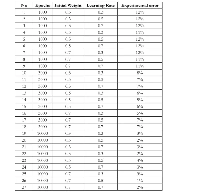
values of the network. Table (5) shows the error rate when
changing the value of the three variables mentioned in Table
(4). The network with the lowest error rate and the lowest error ratio were selected at experiment number 26. Figure (3) shows a
comparison between the real and predicted values of roughness
by the artificial neural network model.
Conclusion
In this study, multiple regression and artificial neural network
approaches were used to predict the surface roughness of alloy steel HRC15. Regarding to the value of P of multiple linear
regression model it can be concluded that the most influential
factor on surface roughness is the amount of feed rate and then
the cutting speed. On the other hand, the depth of cut is the least.
The value of F test signal was much smaller than 0.05 which means that the model is statistically acceptable. The predicted values
obtained from the artificial neural network model were better
than the multiple linear regression model by error of 1% and
20%, respectively. The most significant variable when developing the network in the artificial neural network model was epochs,
where the error rate was 11% at number of iterations 1000 to 1% at number of iterations 10,000. The proposed models can be used effectively to predict the surface roughness in turning process. Considering the advantages of the ANN compared to multiple regression are simplicity, speed, and capacity of learning, the ANN is a powerful approach in predicting the surface roughness.
References
[1]. Asiltürk I, Çunkas M. Modeling and prediction of surface roughness in turning operations using artificial neural network and multiple regression method. Expert systems with applications. 2011 May;38(5):5826-5832. [2]. Rodic D, Gostimirovic M, Kovac P, Radovanovic M, Savkovic B.
Compari-son of Fuzzy logic and neural network for modeling surface roughness in EDM. Intl J Recent advances Mech Eng. 2014 Aug;3(3):69-78.
[3]. Asiltürk I, Neseli S. Multi response optimization of CNC turning parame-ters via Taguchi method based response surface analysis. Measurement. 2012 May;45(4):785-794.
[4]. Ravikumar D, Oza NV, Bhavsar SN. Prediction of surface roughness in CNC milling machine by controlling machining parameters using ANN. Int J Mech Eng Rob. 2014 Oct;3( 4):353-359.
[5]. Parmar JG, Makwana A. Prediction of surface roughness for end milling process using Artificial Neural Network. Intl J Modern Eng Res. 2012
Table 5. Error ratio in the experiments of surface roughness values in ANN model.
No Epochs Initial Weight Learning Rate Experimental error
1 1000 0.3 0.3 12% 2 1000 0.3 0.5 12% 3 1000 0.3 0.7 12% 4 1000 0.5 0.3 11% 5 1000 0.5 0.5 12% 6 1000 0.5 0.7 12% 7 1000 0.7 0.3 12% 8 1000 0.7 0.5 11% 9 1000 0.7 0.7 11% 10 3000 0.3 0.3 8% 11 3000 0.3 0.5 7% 12 3000 0.3 0.7 7% 13 3000 0.5 0.3 6% 14 3000 0.5 0.5 5% 15 3000 0.5 0.7 6% 16 3000 0.7 0.3 5% 17 3000 0.7 0.5 7% 18 3000 0.7 0.7 7% 19 10000 0.3 0.3 3% 20 10000 0.3 0.5 2% 21 10000 0.3 0.7 3% 22 10000 0.5 0.3 2% 23 10000 0.5 0.5 4% 24 10000 0.5 0.7 3% 25 10000 0.7 0.3 3% 26 10000 0.7 0.5 1% 27 10000 0.7 0.7 2%
Jun;2(3):1006-1013.
[6]. Aghdeab SH, Mohammed LA, Ubaid AM. Optimization of CNC Turning for Aluminum Alloy Using Simulated Annealing Method. Jordan J Mech Indust Eng. 2015 Feb;9(1):39 - 44.
[7]. Tsao CC. Grey–Taguchi method to optimize the milling parameters of alu-minum alloy. Intl J Adv Manufac Technol. 2009 Jan;40(1-2):41-48. [8]. Fang N, Srinivasa P, Edwards N. Neural Network Modeling and
Predic-tion of Surface Roughness in Machining Aluminum Alloys. J Comp Comm. 2016 May;4(5):1-9.
[9]. J. Pavan GJ, Narayana L. Prediction of surface roughness in turning process
using soft computing techniques. Int J Mech Eng Rob. 2015 Jan;4(1):561-570.
[10]. Dinesh S, Rajaguru K, Vijayan V. Investigation and Prediction of Material Removal Rate and Surface Roughness in CNC Turning of EN24 Alloy Steel. Mechanics Mechanical Eng. 2016 ;20(4):451-466.
[11]. Lyman O, Longnecker M. An Introduction to Statistical Methods and Data Analysis. 6th ed. USA:Brooks cole; 2008.
[12]. Gurney K. An introduction to Neural Networks. 2nd ed. Taylor & Fran-cis;1991.