Robust Controller Design by Convex Optimization based on Finite
Frequency Samples of Spectral Models
Gorka Galdos, Alireza Karimi and Roland Longchamp
Abstract— Some frequency-domain controller design prob-lems are solved using a finite number of frequency samples. Consequently, the performance and stability conditions are not guaranteed for the frequencies between the frequency samples. In this paper, all possible interpolants between the frequency samples of the open-loop system are bounded using convex constraints on a linearly parameterized controller. These con-straints are integrated in a method which solves anH∞control
problem based on spectral models by convex optimization. The method is applied to a simulation example. It is shown how the added conservatism is reduced while the number of frequency samples is increased.
I. INTRODUCTION
Many difficulties arise when physical laws or identification methods are used to obtain parametric models. Consequently, some controller design methods have been developed based on frequency-domain or time-domain data instead of using parametric models. Frequency-domain data or spectral mod-els are preferred because the stability condition and some performance specifications can be defined in frequency-domain.
Several frequency-domain methods as loop-shaping in Bode diagram, Ziegler-Nichols tuning method and the Quan-titative Feedback Theory [1] are still used in many applica-tions. Although the graphical tools are usually used in these approaches, with new progress in numerical methods for solving optimization problems, new approaches for controller design have been developed [2], [3], [4], [5], [6], [7], [8], [9]. These controller design methods use only a finite number of frequency-domain data to solve the control problem. As a consequence, the stability and performance constraints are only verified at a finite number of frequency samples. Practically, if the number of samples is large enough, this may lead to stable controllers with desired performances. However, in this paper it is shown that, it is possible to satisfy the constraints for all frequencies only using a finite number of frequencies if some assumptions are verified on the system. Nevertheless, the difficulty is to know which is the minimum number of necessary frequencies. The systems behavior between the measured frequency samples is named, in the sequel, the inter-grid behavior.
In [10], the set of all possible interpolants that corresponds to the measured frequency samples is defined with a prior assumption in the impulse response of the system. The
The authors are with the Laboratoire d’Automatique of Ecole Polytech-nique F´ed´erale de Lausanne (EPFL), 1015 Lausanne, Switzerland.
This research work is financially supported by the Swiss National Science Foundation under Grant No. 200020-107872.
Corresponding author:[email protected]
absolute value of the impulse response of the system is assumed to be bounded by a decreasing exponential func-tion that converges to zero. As a result, a bound for the difference between the linear interpolation model and all the possible interpolants between the frequency samples is obtained. This result cannot be applied for systems with integrators because the impulse response cannot be bounded with a decreasing exponential function that converges to zero. A similar problem is treated in [11]. A prior assumption is considered on the relative stability of the underlying system. This means that the real part of the poles of the underlying system are assumed to be greater than a chosen positive value. Then, a frequency dependent bound is given for the all possible interpolants. This reduces slightly the conservatism compared to the previously mentioned constant bound proposed by [10]. These results have been applied to a controller design method presented in [12]. The main drawback of the approach is that non-parametric controllers are obtained. A second step of interpolation is needed to obtain a parametric controller to be applicable in a feedback loop.
In this paper, using some ideas presented in [10], a solution to the theoretical problem of the inter-grid behavior is given for the controller design method presented in [8], [9]. These papers propose an open-loop shaping method with infinity norm constraints on the weighted closed-loop transfer functions. A linearly parameterized controllerKis designed for the system Gsuch that the open-loop transfer function
L=KG is close to a desired open-loop transfer function. With the aim of finding the inter-grid uncertainty, a bound on the impulse response of L is defined. This permits to compute the inter-grid uncertainty bound. This uncertainty defines all the systems describing the inter-grid behavior. Then, this bound is integrated in the original performance and stability constraints of the controller design method. Finally, a linear constraint is added to ensure the imposed bound on the impulse response ofL. This impulse response is calculated only using a finite number of the open-loop frequency response samples. The uncertainty bound are also developed for open-loop systems containing one integrator. The proposed method can be used for PID controllers as well as for higher order linearly parametrized controllers in discrete or continuous time. This approach can also treat the multimodel uncertainty case. The proposed approach is applied in a simulation example showing how the added conservatism is decreased when the number of the frequency samples is increased.
interpolants between the frequency samples of the frequency response of a signal are bounded based on some results of [10] in Section II. Section III introduces this bound for a general controller design problem in Nyquist diagram. The results are applied to the method proposed in [8], [9]. Simulation results are given in IV. Finally, some conclusions are given in Section V.
II. ANALYSIS OF THEINTER-GRID BEHAVIOR
A. Inter-grid uncertainty
Based on the results shown in [10], the frequency sam-ples of a signal are used to define an uncertainty bound. This bound represents all possible interpolants between the samples.
Assume that we have N + 1 samples, X(ωk) for k =
0, . . . , N of the original frequency responseX(ω)between
0 andωmax rad/s spaced by ωmax
N . It is considered that the
frequency response of X(ω) is negligible for frequencies higher thanωmax. Let the linear interpolation modelXλ(ω) be defined as the frequency response between two consecu-tive frequency pointsX(ωk)andX(ωk+1):
Xλ(ω) =λX(ωk) + (1−λ)X(ωk+1) for ωk < ω < ωk+1
(1) whereω is defined as ω=λωk+ (1−λ)ωk+1 and:
λ= ω−ωk+1
ωk−ωk+1 λ∈[0,1] (2)
For a signalX(ω)with an Inverse Fourier Transformx(t) satisfying|x(t)| ≤M β−t, it is shown in [10] that:
|Xλ(ω)−X(ω)| ≤δ (3) where δ= 12M β( (β+ 1) β−1)3 ωk+1−ωk 2 2 =12M β( (β+ 1) β−1)3 ω max 2N 2 (4)
B. How to deal with integrators
If the Laplace transform of a signal contains an integrator, (a pole at zero), the signal cannot be bounded by a decreasing exponential function that converges to zero. In this case, a similar approach can be applied.
In the sequel, it is considered that the Laplace transform of the signal has only one integrator. The frequency response
˜
X(ω)of the signal is given by:
˜
X(ω) = X(ω)
jω (5)
As in Section II-A, the Inverse Fourier Transformx(t)of the signal X(ω) is bounded |x(t)| ≤ M β−t. This bounds
|Xλ(ω)−X(ω)|as in (4). However, now the goal is to find a bound δint for |X˜λ(ω)−X˜(ω)| based on the bound on
|Xλ(ω)−X(ω)|. Note that the linear interpolation model
˜
Xλ(ω)between the frequency samples is defined as:
˜ Xλ(ω) =λX(ωk) jωk +(1−λ) X(ωk+1) jωk+1 for ωk < ω < ωk+1 (6) It is known that |X˜λ(ω)−X˜(ω)| ≤X˜λ(ω)−Xλ(ω) jω +Xλ(ω) jω −X˜(ω) forωk< ω < ωk+1 (7) The following bound is a direct result from the previous subsection: |Xλ(ω) jω −X˜(ω)|= jω1 (Xλ(ω)−X(ω))≤ 1 jωk δ forωk< ω < ωk+1 (8) From (1) and (2), the following equation is obtained:
Xλ(ω) jω = ω−ωk+1 ωk−ωk+1 X(ωk) jω +(1− ω−ωk+1 ωk−ωk+1) X(ωk+1) jω forωk< ω < ωk+1 (9) Then, ifλfrom (2) is replaced in (6) and combined with (9), the following equation is obtained:
X˜λ(ω)−Xλjω(ω) = ωωk−−ωωkk+1+1X(ωk) ωk−ω ωkω − ωk−ω ωk−ωk+1X(ωk+1) ω−ωk+1 ωk+1ω =(ω−ωk+1)(ωk−ω) (ωk−ωk+1)ω X(ωk) ωk − X(ωk+1) ωk+1 forωk< ω < ωk+1 (10) which has a maximum value when ω = √ωkωk+1. Then, (10) can be bounded by:
X˜λ(ω)−Xλjω(ω) ≤( √ω kωk+1−ωk+1)(ωk−√ωkωk+1) (ωk−ωk+1)√ωkωk+1 × X(ωk) ωk − X(ωk+1) ωk+1 =(√ωk−√ωk+1)2 ωk−ωk+1 X(ωk) ωk − X(ωk+1) ωk+1 = ωk−ωk+1 (√ωk+√ωk+1)2 X(ωk) ωk − X(ωk+1) ωk+1 forωk< ω < ωk+1 (11) Replacingωk+1−ωk by ωmax N : X˜λ(ω)−Xλjω(ω) ≤N1 ωmax (√ωk+√ωk+1)2× X(ωk) ωk − X(ωk+1) ωk+1 forωk< ω < ωk+1 (12)
Therefore, the boundδint for the difference between the linear interpolation model X˜λ(ω) and all possible inter-polants between the frequency samples when the frequency
response contains an integrator is given by: δint(ω) = N1 (√ωkω+max√ωk+1)2Xω(ωkk)−Xω(ωkk+1+1) + 1 jωk δ for ωk < ω < ωk+1 (13)
Remark: It should be noted that these bounds are conser-vative but decrease rapidly whileN is increased. For the no integrator case, the boundδ in (4) decreases by a factor of
1/N2while for the case with one integrator, the boundδint in (13) decreases by a factor of1/N.
III. CONTROLLER DESIGN METHOD
The inter-grid behavior of a frequency function can be analyzed following the Sections II-A and II-B. In an open-loop shaping controller design method, X(ω) or X˜(ω) are the open-loop transfer function of the system (a function of the controller parameters). However, the controller is not known a priori, so those results cannot be applied directly. Thus, the results presented in Sections A and II-B should be integrated in a controller design method taking into account the inter-grid behavior in function of controller parameters.
The main idea is to define convex constraints on controller parameters so that the assumption concerning the bounded impulse response is verified. Then, the graphical interpre-tation of the bound for the difference between the linear interpolation model and the frequency samples of the open-loop is used to define new constraints.
The class of stable continuous-time LTI-SISO systems with bounded infinity norm are considered. The system is represented by a spectral modelG(jω).
The objective is to design a linearly parameterized con-troller given by :
K(s, ρ) =ρTφ(s) (14) where
ρT = [ρ1, ρ2, . . . , ρn] (15)
φT(s) = [φ1(s), φ2(s), . . . , φn(s)] (16)
n is the number of controller parameters and φi(s), i =
1, . . . n are stable transfer functions with possible poles on the imaginary axis chosen from a set of orthogonal basis functions. It is clear that PID controllers belong to this set. The main property of this parameterization is that every point on the Nyquist diagram ofK(jω, ρ)G(jω)can be written as a linear function of the controller parametersρ:
K(jω, ρ)G(jω) = ρTφ(jω)G(jω)
= ρTR(ω) +jρTI(ω) (17)
whereR(ω)andI(ω)are respectively the real and imaginary parts ofφ(jω)G(jω).
A. Controller design (no integrator)
The open-loop transfer function of the system is
L(jω, ρ) = K(jω, ρ)G(jω). It is considered that only a finite number of samples of the open-loop frequency response L(jωk, ρ) for k = 0, . . . , N are available. The
inter-grid behavior of the open-loop frequency response depends on the impulse response of the open-loop (t, ρ). This impulse response can be computed with the Inverse Fourier Transforme using the open-loop frequency response
L(jω, ρ):
(t, ρ) = ∞
−∞L(jω, ρ)e
jωtdω (18)
Note that, L(jω, ρ) can be exactly calculated using only the available N+ 1 finite number of samples of the open-loop frequency responseL(jωk, ρ), if the Dual of Shannon’s
Theorem is satisfied. In the Theorem given in Appendix A, it is shown that the uniformly spaced discrete samples of the frequency response of a signal are a complete representation of the frequency response if the impulse response obtained by its Inverse Fourier Transform is a time-limited signal.
The impulse response in (18) can be approximated based on the Inverse Discrete Fourier Transforme usingN+1 open-loop frequency response samples:
(hTs, ρ) = 1 N+ 1 N k=0 L(jωk, ρ)ejωkhTs forh= 0, . . . , N (19) whereTs= ωπ
max. Then,(hTs, ρ)can be bounded with the following convex constraints:
(hTs, ρ)≤M β−hTs forh= 0, . . . , N (20)
(hTs, ρ)≥ −M β−hTs forh= 0, . . . , N (21)
Note that the constraints are linear because the controller to be designed is linearly parameterized. Now, the inter-grid behavior can be defined for all ω using the constant bound given in (4). It should be noted that this bound is defined around the following linear interpolation model:
Lλ(ω, ρ) =λL(jωk, ρ) + (1−λ)L(jωk+1, ρ)
for ωk < ω < ωk+1 (22)
Below, the main idea of fixed-orderH∞controller design for SISO systems proposed in [9] is reviewed. For simplic-ity, an open-loop shaping controller design problem with constraint on one weighted closed-loop sensitivity function is considered. The 2-norm of L−Ld is minimized under the closed-loop sensitivity function conditionW1S∞<1 whereS = (1 +L)−1.
In [9] it is shown that the constraintW1S∞<1can be approximated by the following linear constraint:
|W1(jω)[1 +Ld(jω)]|−
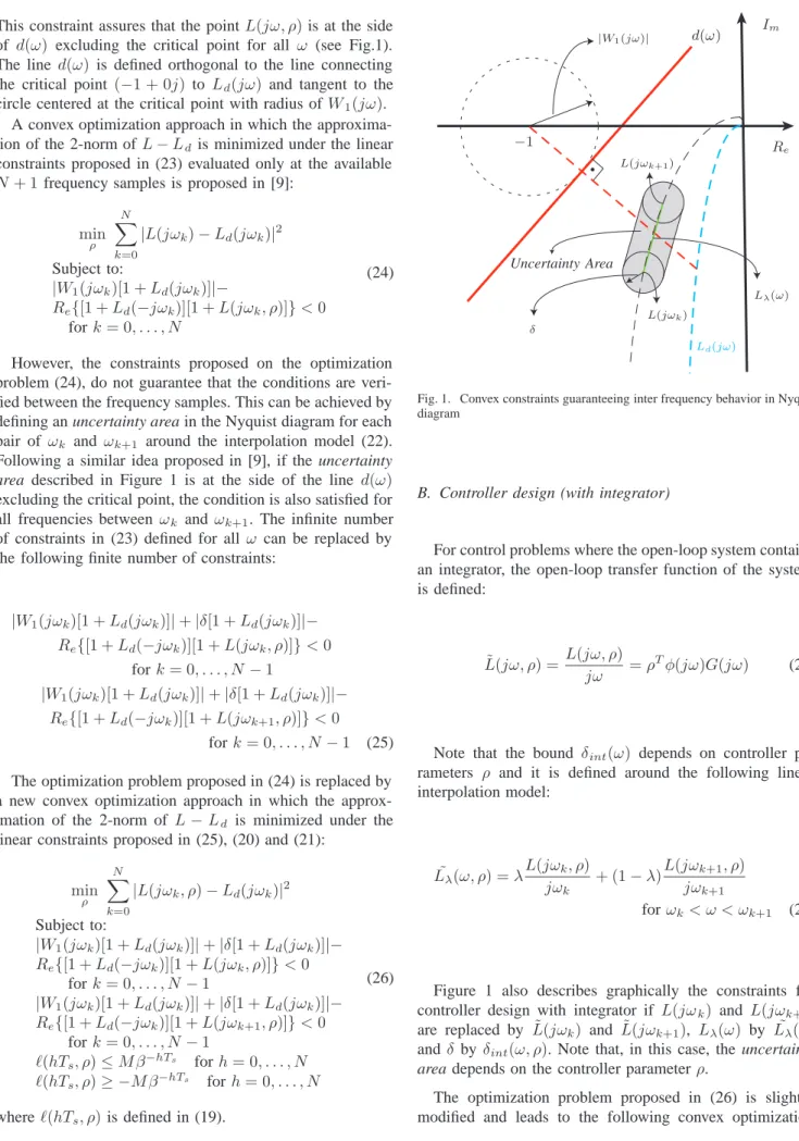
This constraint assures that the pointL(jω, ρ)is at the side of d(ω) excluding the critical point for all ω (see Fig.1). The line d(ω) is defined orthogonal to the line connecting the critical point (−1 + 0j) toLd(jω) and tangent to the circle centered at the critical point with radius ofW1(jω).
A convex optimization approach in which the approxima-tion of the 2-norm ofL−Ld is minimized under the linear constraints proposed in (23) evaluated only at the available
N+ 1 frequency samples is proposed in [9]:
min ρ N k=0 |L(jωk)−Ld(jωk)|2 Subject to: |W1(jωk)[1 +Ld(jωk)]|− Re{[1 +Ld(−jωk)][1 +L(jωk, ρ)]}<0 fork= 0, . . . , N (24)
However, the constraints proposed on the optimization problem (24), do not guarantee that the conditions are veri-fied between the frequency samples. This can be achieved by defining an uncertainty area in the Nyquist diagram for each pair of ωk and ωk+1 around the interpolation model (22).
Following a similar idea proposed in [9], if the uncertainty
area described in Figure 1 is at the side of the line d(ω)
excluding the critical point, the condition is also satisfied for all frequencies between ωk andωk+1. The infinite number
of constraints in (23) defined for all ω can be replaced by the following finite number of constraints:
|W1(jωk)[1 +Ld(jωk)]|+|δ[1 +Ld(jωk)]|− Re{[1 +Ld(−jωk)][1 +L(jωk, ρ)]}<0 fork= 0, . . . , N−1 |W1(jωk)[1 +Ld(jωk)]|+|δ[1 +Ld(jωk)]|− Re{[1 +Ld(−jωk)][1 +L(jωk+1, ρ)]}<0 fork= 0, . . . , N−1 (25) The optimization problem proposed in (24) is replaced by a new convex optimization approach in which the approx-imation of the 2-norm of L−Ld is minimized under the
linear constraints proposed in (25), (20) and (21):
min ρ N k=0 |L(jωk, ρ)−Ld(jωk)|2 Subject to: |W1(jωk)[1 +Ld(jωk)]|+|δ[1 +Ld(jωk)]|− Re{[1 +Ld(−jωk)][1 +L(jωk, ρ)]}<0 for k= 0, . . . , N−1 |W1(jωk)[1 +Ld(jωk)]|+|δ[1 +Ld(jωk)]|− Re{[1 +Ld(−jωk)][1 +L(jωk+1, ρ)]}<0 for k= 0, . . . , N−1 (hTs, ρ)≤M β−hTs for h= 0, . . . , N (hTs, ρ)≥ −M β−hTs forh= 0, . . . , N (26) where(hTs, ρ)is defined in (19). |W1(jω)| δ Ld(jω) L(jωk) d(ω) Re Im L(jωk+1) −1 Lλ(ω) Uncertainty Area
Fig. 1. Convex constraints guaranteeing inter frequency behavior in Nyquist diagram
B. Controller design (with integrator)
For control problems where the open-loop system contains an integrator, the open-loop transfer function of the system is defined:
˜
L(jω, ρ) =L(jω, ρ) jω =ρ
Tφ(jω)G(jω) (27)
Note that the bound δint(ω) depends on controller pa-rameters ρ and it is defined around the following linear interpolation model: ˜ Lλ(ω, ρ) =λL(jωk, ρ) jωk + (1−λ) L(jωk+1, ρ) jωk+1 for ωk < ω < ωk+1 (28)
Figure 1 also describes graphically the constraints for controller design with integrator if L(jωk) and L(jωk+1) are replaced by L˜(jωk) and L˜(jωk+1), Lλ(ω) by L˜λ(ω) andδ byδint(ω, ρ). Note that, in this case, the uncertainty
area depends on the controller parameterρ.
The optimization problem proposed in (26) is slightly modified and leads to the following convex optimization
problem: min ρ N k=0 |L˜(jωk, ρ)−Ld(jωk)|2 Subject to: |W1(jωk)[1 +Ld(jωk)]|+|δint(ωk, ρ)[1 +Ld(jωk)]|− Re{[1 +Ld(−jωk)][1 + ˜L(jωk, ρ)]}<0 for k= 0, . . . , N −1 |W1(jωk)[1 +Ld(jωk)]|+|δint(ωk, ρ)[1 +Ld(jωk)]|− Re{[1 +Ld(−jωk)][1 + ˜L(jωk+1, ρ)]}<0 for k= 0, . . . , N −1 (hTs, ρ)≤M β−hTs for h= 0, . . . , N (hTs, ρ)≥ −M β−hTs for h= 0, . . . , N (29) where δint(ωk, ρ) = N1(√ωkω+max√ωk+1)2L(jωωkk,ρ)−L(jωωkk+1+1,ρ) + 1 jωk (30) and(hTs, ρ)is computed based on the open-loop transfer functionL(jωk, ρ)(which does not contain the integrator).
It should be noted that the optimization problem proposed in (26) contains only linear constraints while that proposed in (29) contains linear and convex constraints. The optimization problem in (26) can be solved very efficiently even with thousand of constraints by standard quadratic programming. On the other hand, an SDP solver is needed to solve the optimization problem in (29) (e.g. SeDuMi [13]).
IV. SIMULATION RESULTS
A simulation example is presented in this section where a PD controller is designed. The idea is to show how the conservatism is reduced when the number of frequency samples is incresed.
The following continuous-time transfer function system is considered:
G(s) =( 1
s+ 1)(s+ 2) (31)
for which the following PD controller should be tuned:
K(s) = ρ1s0 +ρ0
.1s+ 1 (32)
The goal is to design a controller minimizing the 2-norm of
L−Ldwith a modulus margin of at least 0.5 (W1(s) = 0.5)
where Ld(s) = s+11 is chosen. The impulse response of
Ld(s) is e−t. However, β and M are chosen 10% higher
than those values, giving β = 1.1 and M = 1.1. The frequency response of Ld(s) is negligible for frequencies higher than100rad/s, hence,ωmax= 100rad/s is chosen. It should be noted that the computation of the impulse response of the open-loop system is not accurate for high values of h. Therefore, only the constraints bounding the impulse response for which the boundM β−hTs is higher than10−3 are considered.
The optimization problem presented in (26) is solved with N + 1 equally spaced frequency samples between 0
TABLE I
WITH INTER-GRID CONDITION
N+ 1 L−Ld2 ρ1 ρ0 T C [s] 100 Not feasible 1000 Not feasible 10000 0.2625 1.2094 1.2371 21 100000 0.1961 1.2000 1.8462 814 TABLE II
WITHOUT INTER-GRID CONDITION N+ 1 L−Ld2 ρ1 ρ0 T C [s]
100 0.1967 1.2000 1.8978 0.82 1000 0.1961 1.2000 1.8533 0.81 10000 0.1961 1.2000 1.8469 2.4 100000 0.1961 1.2000 1.8462 169
and ωmax rad/s for different values of N. The results are shown in Table I forN+ 1equal to 100, 1000, 10000 and 100000. It can be seen that the 2-norm ofL−Ldis reduced when N is increased. This result is expected because the inter-grid uncertainty δ is decreasing when N is increased which reduces de conservatism of the approach. However, the computational cost (T C) is as well increased.
As expected, if the same control problem is solved based on the optimization problem proposed in (24), better per-formances can be obtained for the same number of data
N+ 1. The results are shown in Table II. Note that using the approach proposed in this paper, if N is large enough, the results are the same as those obtained with the method not considering the inter-grid uncertainty.
V. CONCLUSION
A solution for the inter-grid behavior to verify the stability and performance condition for frequency-domain controller design methods has been presented. Convex constraints are proposed to bound the impulse response of the open-loop system. This allows to do smoothness assumptions which are used to bound the difference between the linear interpolation model and all possible interpolants between the frequency samples of the open-loop system. Additionally, it is shown how this bound is reduced when the number of frequency samples is increased. These results are integrated in anH∞ controller design method where a linearly parameterized con-troller is designed by convex optimization. The simulation result show that using a finite number of frequency samples, the stability and performance conditions can be satisfied even for frequencies between the samples if a conservatism is added. This conservatism decreases if the number of frequency samples increases. Consequently, the complexity of the problem increases. Same results can be obtained with much less computational complexity only verifying the constraints at the available frequency samples. It should be noted that in this case, there is no guarantee that the conditions are verified between the frequency samples.
REFERENCES
[1] I. M. Horowitz. Quantitative Feedback Theory (QFT). QFT Publica-tions Boulder, Colorado, 1993.
[2] G. F. Bryant and G. D. Halikias. Optimal loop shaping for systems with large parameter uncertainty via linear programming. International
Journal of Control, 62:557–568, 1995.
[3] Y. Chait, Q. Chen, and C. V. Hollot. Automatic loop-shaping of QFT controllers via linear programming. Journal of Dynamic Systems,
Measurement and Control, 121(3):351–357, September 1999.
[4] G. D. Halikias, A. C. Zolotas, and R. Nandakumar. Design of optimal robust fixed-structure controllers using the quantitative feedback theory approach. Proceedings of the Institution of Mechanical Engineers, Part
I: Journal of Systems and Control Engineering, 221(4):697–716, 2007.
[5] E. Grassi and K. Tsakalis. PID controller tuning by frequency loop shaping. In 35th IEEE Conference on Decision and Control, pages 4776–4781, Kobe, Japan, 1996.
[6] E. Grassi, K. S. Tsakalis, S. V. Gaikwad S. Dash, W. MacArthur, and G. Stein. Integrated system identification and PID controller tuning by frequency loop-shaping. IEEE Transactions on Control Systems
Technology, 9(2):285–294, 2001.
[7] A. Karimi, M. Kunze, and R. Longchamp. Robust controller design by linear programming with application to a double-axis positioning system. Control Engineering Practice, 15(2):197–208, February 2007. [8] G. Galdos, A. Karimi, and R. Longchamp. Robust loop shaping controller design for spectral models by quadratic programming. In
46th IEEE Conference on Decision and Control, pages 171–176, New
Orleans, USA, 2007.
[9] A. Karimi, G. Galdos, and R. Longchamp. Robust fixed-orderH∞
controller design for spectral models by convex optimization. In 47th
IEEE Conference on Decision and Control, Cancun, MEX, 2008.
[10] D. de Vries. Identification of Model Uncertainty for Control Design. PhD thesis, Delft University of Technology, Delft, The Netherlands, 1994.
[11] A.J. den Hamer, S. Weiland, and M. Steinbuch. Worst-case inter frequency grid behavior of transfer functions identified via finite frequency response data. In European Control Conference, pages 466– 471, Budapest, Hungary, 2010.
[12] A.J. den Hamer, S. Weiland, M. Steinbuch, and G.Z. Angelis. Stability and causality constraints on frequency response coefficients applied for non-parametric h2 and h∞control synthesis. In Conference on
Decision and Control, pages 3670–3675, Cancun, Mexico, 2008.
[13] J. F. Sturm. Using SeDuMi 1.02, a Matlab toolbox for optimization over symmetric cones. Optimization Methods and Software, 11:625– 653, 1999.
APPENDIX
A. Dual of Shannon’s Theorem
According to Shannon’s Sampling Theorem, the uniformly spaced discrete samples of a time-domain signal are a com-plete representation of the signal if its sampling rate is higher than the double of the signal’s bandwidth. Similarly, the uniformly spaced discrete samples of the frequency response of a signal are a complete representation of the frequency response if the impulse response obtained by its Inverse Fourier Transform is time limited.
Theorem: X(ω) is completely determined by its ordinates at a series of points spaced by less than or equal to π/T if its Inverse Fourier Transformx(t) is 0 for t < −T and
t > T.
Proof:x(t)has non 0 values for a period of2T. Therefore, it can be represented as a Fourier series expansion using any periodTm≥2T. The Fourier Transform expansion ofx(t)
can be written as:
x(t) = ∞ k=−∞ Akejk2π t Tm (33) where Ak = T1 m Tm 2 −Tm 2 x(t)e −jk2π t Tmdt. As x(t) is 0 for
t <−Tmandt > Tm, the Fourier Transform is reduced to:
X(ω) =F{x(t)}= ∞ −∞x(t)e −jωtdt= Tm −Tm x(t)e−jωtdt (34) By comparison, Ak = T1 mX(k 2π
Tm). Hence, this implies thatX(ω)can be fully represented by its samples.
X(ω) = 1 Tm Tm −Tm ∞ k=−∞ X(ωk)ejk2πTmt e−jωtdt (35) whereωk=kT2π m.