New developments in causal inference using balance optimization subset selection

(1)

c

(2)

NEW DEVELOPMENTS IN CAUSAL INFERENCE USING BALANCE OPTIMIZATION SUBSET SELECTION

BY

HEE YOUN KWON

DISSERTATION

Submitted in partial fulfillment of the requirements

for the degree of Doctor of Philosophy in Systems and Entrepreneurial Engineering in the Graduate College of the

University of Illinois at Urbana-Champaign, 2018

Urbana, Illinois

Doctoral Committee:

Assistant Professor Niao He, Chair

Professor Sheldon H. Jacobson, Director of Research Assistant Professor Karthekeyan Chandrasekaran Professor Rakesh Nagi

(3)

ABSTRACT

Causal inference with observational data has drawn attention across various fields. These observational studies typically use matching methods which find matched pairs with similar covariate values. However, matching methods may not directly achieve covariate balance, a measure of matching effectiveness. As an alternative, the Balance Optimization Subset Selection (BOSS) framework, which seeks the optimal covariate balance directly, has been proposed. This dissertation extends the BOSS framework in various ways and is composed of the following five parts. The first part of the dissertation investigates all the possible cases that may lead to bias in the context of BOSS and tries to mitigate the bias. Second, this dissertation then extends the BOSS by estimating and decomposing a treatment effect as a combination of heterogeneous treatment effects from a partitioned set using the BOSS. Third, the dissertation generalizes the BOSS framework from a binary treatment setting to a multi-treatment setting. A treatment effect estimate with multiple treatments can be computed by combining estimates obtained from BOSS with binary treatments. The fourth part discusses on how to handle missing data with BOSS. It includes a sensitivity analysis of BOSS studying how the esti-mated values are affected by violation of the conditional independence assumption and methods to apply BOSS after multiple imputation on missing covariates. In these discussions, the performances of BOSS estimators are compared to those of matching estimators. In the last part, BOSS is formulated as an LP by relax-ing integer constraints in the original mixed integer programmrelax-ing formulation and properties of its dual problem are investigated.

(4)

(5)

ACKNOWLEDGMENTS

The very first person that I would like to mention is my PhD advisor, Professor Sheldon H. Jacobson. I am very fortunate to have him as my advisor and really grateful for invaluable advice that he has provided me over the last several years. I am hugely indebted to his insightful guidance and thoughtful encouragement throughout my PhD study in Systems and Entrepreneurial Engineering at the Uni-versity of Illinois at Urbana-Champaign.

I am also very grateful for my PhD Final Examination (Defense) Committee members – Professor Karthik Chandrasekaran, Professor Niao He, and Professor Rakesh Nagi – and Professor Jason J. Sauppe who gave me a lot of feedback when I was working on this research. I would like to express my gratitude to Professor Negar Kiyavash as well for being my Preliminary Examination Committee mem-ber and I thank Professor Alex Olshevsky and Professor Sewoong Oh for being my first year advisors at Illinois.

I would like to thank my MPhil advisor Professor Sujoy Mukerji and Professor Marcel Fafchamps for their help when I was transitioning from an MPhil stu-dent in economics at the University of Oxford to a PhD stustu-dent in engineering at Illinois. I am grateful to Professor Gyo Taek Jin, Professor Sang-il Oum, Profes-sor Yoon-Jae Whang, ProfesProfes-sor Elias Sanidas and ProfesProfes-sor Roland Herzog who provided support and guidance when I was starting an intellectual journey as a graduate student.

Additionally, my thanks should go to the Mavis Fellowship program from Col-lege of Engineering at Illinois for providing a great training opportunity in addi-tion to the financial support. Financial support in the form of research and teaching assistantship from Department of Industrial and Enterprise Systems Engineering (ISE)· Computational Science and Engineering Program (CSE)· Department of Computer Science (CS) at Illinois is gratefully acknowledged. I also highly ap-preciate Samsung Scholarship Foundation which provided me a generous support during my master’s study and the University of Oxford for its institutional support

(6)

when I was an MPhil student. I would have not been able to finish my graduate study without the support from these institutions and academic advisors.

I also would like to thank Ms. Holly Kizer, Ms. Aleta Lynch, and Ms. Elaine Wilson for their administrate support. Furthermore, I cannot list all of their names but I am really grateful to the current and former members of the Simulation and Optimization Laboratory and many other friends who helped me in various ways. Lastly, I thank my family members – my parents, younger sister and younger brother. They have provided me an unceasing encouragement. This dissertation is dedicated to my family.

A part of this dissertation has been published in the Journal of the Operational Research Society.

(7)

TABLES

2.1 Relationship between objective function value and the bias . . . . 17

3.1 One-sided p-values of the Estimated Average Treatment Ef-fects for the Treated . . . 52

3.2 One-sidedp-values when Bootstrap Hypothesis Testing is Con-ducted to Respective Treatment Effects . . . 61

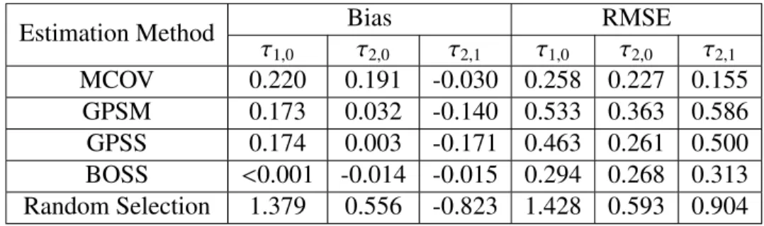
4.1 Comparison of Estimators (The First Experiment) . . . 76

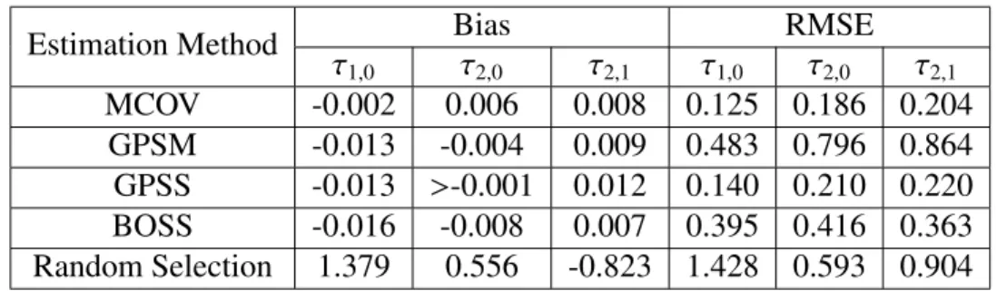
4.2 Comparison of Estimators (The Second Experiment) . . . 78

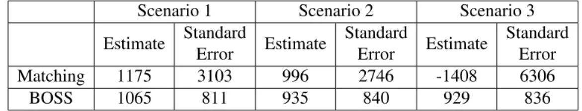
5.1 Simulation Results under Three Scenarios . . . 90

5.2 Matching Estimators (and Corresponding Standard Errors) . . . . 91

5.3 BOSS Estimators (and Corresponding Standard Errors) . . . 91

5.4 Values of (p11,p10,p01,p00) under Each Scenario . . . 104

5.5 Matching Estimators (and Corresponding Standard Errors) . . . . 106

5.6 BOSS Estimators (and Corresponding Standard Errors) . . . 107

5.7 Values of (p11,p10,p01,p00) under Each Scenario . . . 108

5.8 Propensity Score Matching Estimators after multiple imputa-tion withL= 5 and 100 repetitions . . . 110

5.9 BOSS Estimators after multiple imputation with L = 5 and 100 repetitions . . . 110

6.1 Changing the RHS of the First Constraint in (6.18) . . . 118

6.2 Changing the RHS of the Second Constraint in (6.18) . . . 119

6.3 Changing the RHS of the Third Constraint in (6.18) . . . 119

(10)

FIGURES

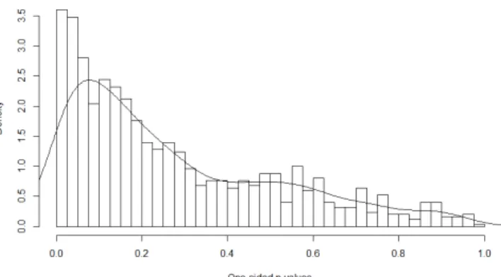
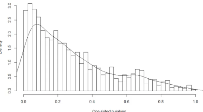
2.1 Balance Hierarchy Example . . . 20 2.2 Another Balance Hierarchy Example . . . 24 2.3 Range of Covariate Values . . . 35 3.1 Histogram and Density of 1000p-values of Bootstrap

Hypoth-esis Testing with a Treatment Group from Experimental NSW Treatment Data and the Corresponding Control Group from

Experimental NSW Control Data . . . 58 3.2 Histogram and Density of 1000p-values of Bootstrap

Hypoth-esis Testing with a Treatment Group from Experimental NSW Treatment Data and the Corresponding Control Group from

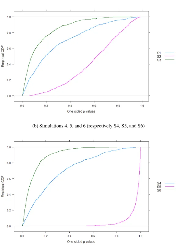
Non-experimental PSID Control Data . . . 59 3.3 Empirical CDF of One-sided p-values . . . 60 5.1 Graphical Representation of (p11,p10,p01,p00) Values under

36 Scenarios in Table 5.4 . . . 105 5.2 Graphical Representation of (p11,p10,p01,p00) Values under

(11)

ABBREVIATIONS

BOSS Balance Optimization Subset Selection ATE Average treatment effect

ATT Average treatment effect for the treated

LP Linear programming

MIP Mixed integer programming GMD Generalized Mahalanobis distance DOM Difference of means

DOM+DOV Difference of first and second moments DOM2 Bivariate moment

KS Kolmogorov-Smirnov test statistic

ecdf Empirical cumulative distribution function CvM Cramer-von Mises test statistic

CPU Central processing unit

GHz Gigahertz

NSW National Supported Work Demonstration program PSID Population Survey of Income Dynamics

RE74 Real earnings in year 1974 RE75 Real earnings in year 1975 RE78 Real earnings in year 1978

(12)

S2 Scenario 2

S3 Scenario 3

S4 Scenario 4

S5 Scenario 5

S6 Scenario 6

U74 Unemployment rate in year 1974 MSE Mean squared error

RMSE Root mean squared error

MCOV Nearest neighbor covariate matching GPSM Generalized propensity score matching

GPSS Sub-classification on the generalized propensity score MCAR Missing completely at random

MAR Missing at random

MNAR Missing not at random

Pri.DE Pediatric Respiratory Infection in Deutschland RSV Respiratory Syncytial Virus

LRTI Lower Respiratory Tract Infections

(13)

NOTATION

u Unit

U Population; Set of all possible units (Note: u∈ U)

Zu Treatment level of unitu∈U

Z Treatment level of a a unit selected randomly from populationU where the random selection is uniform

L Number of treatment levels

L=2 in a binary treatment setting and

L≥2 in a multi-treatment setting L Set of treatment levels

L ={0,1,· · · ,L−1} (Note: U= {u:Zu∈ L})

Ui _{Set of units in population whose treatment level is}_i Ui ={u∈U :Zu =i}fori∈ L

(Note: U =U0∪U1∪ · · · ∪UL−1)

Si _{Samples drawn from}_Ui _for_i_{∈ L} t Treated unit

c Control unit; Untreated unit

T Treatment group; Set of all the treated units

T = S1under a binary treatment setting

C Control pool; Set of all the control units

C =S0under a binary treatment setting

C0 Control group; Set of control units selected from the control pool under a binary treatment setting

(14)

N Number of observed units

N =|T|+|C0|under a binary treatment setting

N =|S0_|+_|_S1_|+_{· · ·}+_|_SL−1_|_{under a multi-treatment setting} N Set of all the observed units

N ={u1,· · · ,uN}

N =T ∪C under a binary treatment setting

N =S0∪S1∪ · · · ∪SL−1 =∪L−_i₌₀1Siunder a multi-treatment setting

S Set of some observed units (Note: S ⊂ N)

Xu,k Thek-th covariate value of unitu∈U K Number of covariate indices

P Set of all covariate indices P={1,2,· · · ,K}

K Set of some covariate indices (Note: K ⊂ P)

D Set of all possible clusters of covariate indices; Power set ofP

Xu Vector of covariates of unitu∈ U

Xu =(Xu,1,Xu,2,· · · ,Xu,K)

X Vector of K covariate values for a unit selected randomly from populationU where the random selection is uniform

X Set of possible values forX(Support ofX)

Xk(S) Set of possible values for thek-th covariate value for all unitsu∈S

Xk(S)= {Xu,k :u∈S}

I Imbalance measure

(Note: Under a binary treatment setting, it denotes an imbalance measure between a treatment group T and a control groupC0 _for

all covariates whose incides are inPif not noted otherwise.) IDOM Imbalance measure balancing the difference of means

Under a binary treatment setting, the imbalance measure between setsG1andG2is given by

IDOM(G1,G2)= P K k=1 1 |G1| P u∈G1Xu,k− 1 |G2| P u∈G2 Xu,k

Under a multi-treatment setting, IDOM Sl,(Sl)0,(Sl)00,Sm,(Sm)0,(Sm)00= IDOMSl,(Sm)0+ IDOM Sm,(Sl)0+IDOM S−,(Sm)00+IDOM S−,(Sl)00

(15)

IDOM:K Imbalance measure balancing the difference of means for

covari-ates whose indices are inK

IDOM:K(G1,G2)= Pk∈K 1 |G1| P u∈G1 Xu,k− 1 |G2| P u∈G2Xu,G2

IDOM+DOV Imbalance measure balancing the difference of first and second moments

IDOM+DOV(G1,G2)=IDOM+PkK=1

1 |G1| P u∈G1 Xu,k 2₋ 1 |G2| P u∈G2 Xu,k 2

Under a multi-treatment setting, IDOM+DOV Sl,₍_Sl₎0_, (Sl₎00_, Sm,₍_Sm₎0_, (Sm₎00₌ _IDOM +DOV Sl,₍_Sm₎0₊ IDOM+DOV Sm,(Sl)0+IDOM₊DOV S−,(Sm)00+IDOM₊DOV S−,(Sl)00 _P 2

Set of all the possible covariate index pairs

_P

2

={(k1,k2)|k1,k2 ∈ P}

IDOM2 Imbalance measure balancing the bivariate moment

IDOM2(G1,G2)= IDOM+DOV(G1,G2)+

P (k1,k2)∈(P₂) 1 |G1| P u∈G1 Xu,k1Xu,k2 − 1 |G2| P u∈G2Xu,k1Xu,k2

Under a multi-treatment setting, IDOM2 Sl,₍_Sl₎0,₍_Sl₎00,_Sm,₍_Sm₎0,₍_Sm₎00= IDOM2_Sl,₍_Sm₎0+ IDOM2 Sm,₍_Sl₎0₊_IDOM2 S−,(Sm₎00₊_IDOM2 S−,(Sl₎00

ICorr:K Imbalance measure balancing the correlation terms of the form Q

k∈K(Xu,k)pk for covariates whose indices are inK and pk ∈R

ICorr:K(G1,G2)= Pk∈K 1 |G1| P u∈G1 Q k∈K(Xu,k)pk − _|G1 2| P u∈G2 Q k∈K(Xu,k)pk b

Fk(T,x) Empirical distribution function of the treatment groupT b Fk(T,x)= u∈T :Xu,k ≤ x /|T| b

Fk(C0,x) Empirical distribution function of the control groupC0 b Fk(C0,_x₎= u∈C0 _: _Xu ,k ≤ x /|C 0_|

IKS Imbalance measure balancing the Kolmogorov-Smirnov test statis-tic

(16)

IKS(G1,G2)=PkK=1maxx∈Xk(G1∪G2) Fkb(G1,x)−Fkb(G2,x)

Under a multi-treatment setting, IKS

Sl,₍_Sl₎0,₍_Sl₎00,_Sm,₍_Sm₎0,₍_Sm₎00 =IKS_Sl,₍_Sm₎0+

IKS

Sm,₍_Sl₎0+IKS_S−,₍_Sm₎00+IKS_S−,₍_Sl₎00

Iecdf:D Imbalance measure balancing the difference of joint empirical

cu-mulative distribution functions of clusters inDusing the Kolmogorov-Smirnov test statistic

Iecdf:D(G1,G2)=PD∈Dmaxx∈XD(G1∪G2) FDb (G1,x)−FDb (G2,x)

Under a multi-treatment setting, Iecdf:D Sl,₍_Sl₎0,₍_Sl₎00,_Sm,₍_Sm₎0,₍_Sm₎00=Iecdf: D Sl,₍_Sm₎0+ Iecdf:D Sm,₍_Sl₎0₊_Iecdf: D S−,(Sm₎00₊_Iecdf: D S−,(Sl₎00

ICvM Imbalance measure balancing the Cramer-von Mises test statistic Under a binary treatment setting,the imbalance measure between setsG1andG2is given by

Iecdf:D(G1,G2)= |G1|·|G2| (|G1|+|G2|)2 PK k=1 _P x∈Xk(G1∪G2)(Fkb(G1,x)−Fkb(G2,x)) 2 ICvM:D Imbalance measure balancing the difference of joint empirical

cu-mulative distribution functions of clusters inD using the Cramer-von Mises test statistic

ICvM:D(G1,G2)= |G1|·|G2| (|G1|+|G2|)2 P D∈D _P x∈XD(G1∪G2)(FDb (G1,x)−FDb (G1,x)) 2

Nk Set of values that thek-th covariate can have

Ek,j Set of units inN whosek-th covariate is equal to j

ηk,j(G) Number of units inGwhosek-th covariate is equal to j

ηk,j(G)= |Ek,j∩G|forG ∈ {T,C0}

IK Imbalance measure forK using binning

Under a binary treatment setting, IK(T,C0)=Pk∈K

P

j∈Nk|ηk,j(T)−ηk,j(C 0

)|

Mk Set of histogram bin indices for covariatek

Bk,b Set of units whosek-th covariate value is in theb-th bin forb∈ Mk

Ihist Imbalance measure forPusing histogram binning Under a binary treatment setting,

Ihist(T,C0)=PK k=1 P b∈Mk |T∩Bk,b| |T| − |C0_∩B k,b| |C0_|

(17)

hz(Xu) Response function foruin treatment levelz

Under a binary treatment setting, h1(Xu) denotes a treatment

re-sponse functionh0₍_X

u) denote a control response function

z

u Error term in a responses for treatment levelzof a unitu Yz

u Response of unitufor treatment levelz Yz

u =h z₍_X

u)+uzforz∈ L

(Note: Under a binary treatment setting, Yu1 is a treated response

value which is observable for u ∈ T and unobservable for u ∈ C

whileY0

u is a control response value which is observable foru∈C

and unobservable foru∈T. )

E(Yz) Average population response for treatment levelz

τ1 _{Population average treatment e}_ff_{ect for the treated (PATT) under a} binary treatment setting

τ1=

E[Y1−Y0|Z =1]

τ1

T Sample average treatment effect for the treated (SATT) under a

binary treatment setting τ1 T = 1 |T| P t∈T Y1 t −Yt0 eτ 1 T(C 0

) BOSS Estimator of SATTτ1_T in a binary treatment setting

eτ 1 T(C 0₎= 1 |T| P t∈TYt1− 1 |C0_| P c∈C0Y0 c

τ(m,l) Population average treatment effect (PATE) between treatment level

land treatment levelm

τ(m,l)= E[Ym]−E[Yl]

τm,l Sample average treatment effect (SATE) between treatment levell

and treatment levelm

τm,l = _|S1_|Pu∈S Ym u −Y l u =τm,l = _|S0_|₊_|S1_|₊1_···₊_|SL−1_| PL−1 i=0 P u∈Si Ym u −Y l u

ν(m,l) Population average treatment effect which only considers a pair of treatment levels under a multi-treatment setting

ν(l,m)=E[Ym|Z ∈ {l,m}]−E h

Yl _|_Z_{∈ {}_l,_m_}i

ˆ

ν(m,l) Estimator ofν(l,m)

eτBOS S(m,l) BOSS estimator ofE[τm,l] eτBOS S(m,l)=

1

|N |

n_P

u∈(Sm₎0Y_um−P_u∈SlY_ul +P_u∈SmY_um−P_u∈₍_Sl₎0Y_ul +

P u∈(Sm₎00Ym u − P u∈(Sl₎00Yl u o f(u, j) f(u, j)=arg minv:Zv=j||Xv−Xu||

eτGNN(m,l) Generalized Nearest Neighbor covariate matching estimator ofτ(m,l)

eτGNN(m,l)= 1 |N | P u∈N Ym f(u,m)−Y l f(u,l)

(18)

p(z|Xu) Generalized propensity score for a unituwhose covaraite vector is

given byXu

p(j| x)=Prob(Zv = j|Xv = x)

g(u, j) g(u, j)= arg minv:Zv=j|p(j|Xv)−p(j|Xu)|

eτGPS(m,l) Generalized Propensity Score (GPS) matching estimator ofτ(m,l)

eτGPS(m,l)]= 1 |N | P u∈N Y_gm₍_u_,_m₎−Y_gl₍_u_,_l₎ Y1

T Average treated response of units in a treatment groupT

Y_C00 Average untreated (control) response of units in a control groupC

0

P Partition ofT

P ={T1,T2,· · · ,TP}

B(T,C0) Bias term in the estimator_eτ1_T(C0) forτ1_T B(T,C0)= _|T1_|P

t∈Th0(Xt)− _|C10_|

P

c∈C0h0(X_c)

E(T,C0₎ _{Error term in the estimator}

eτ 1 T(C 0_{) for}τ1 T E(T,C0)= _|T|1 P t∈Tt0− |C10_| P c∈C0_c0 B B(T,C0)− |T1| |T|B(T,C 0 1)− |T2| |T|B(T2,C 0 2) E E(T,C0)− |T1| |T|E(T1,C 0 1)− |T2| |T|E(T2,C 0 2) A Set of treated responses for units inT

A ={Y1

t |t∈T}

B Set of untreated responses for units inC0

B = {Y_c0|c∈C0}

µ_A Mean of observed responses inA µ_A =Y1 T = 1 |T| P t∈TYt1

µ_B Mean of observed responses inB µ_B =Y0 C0 = _|C10_| P c∈C0Y0 c H0 Null hypothesis H1 Alternative hypothesis

M Number of iterations in the bootstrap procedure δ Difference in means of elements inAandB

δ =Y1

T −Y

0

C0

Γ Set of observed responses of units inT andC0

Γ = A ∪B ={Y1

t |t∈T} ∪ {Yc0|c∈C 0_}

(19)

Y_T1_,_m Set of|T|observations drawn fromΓin them-th iteration

Y0

C0_,_m Set of|C

0_|

observations drawn fromΓin them-th iteration

Y_T1_,_m Mean of observed values inY_T1_,_m Y_C00_,_m Mean of observed values inY_C00_,_m

δm δm= Y1

T,m−Y 0

C0_,_m in them-th iteration

p p-value for the one-sided hypothesis testH0 versusH1

p=

PM

m=11[δm≥δ]

M in one-sided hypothesis testing

p=

PL

l=11[|δm|≥|δ|]

M in two-sided hypothesis testing

U Previously unobserved binary covariate variable

U Set of the new binary valuesUthat is attached to the given data to form an augmented set of covariates

pi j Prob{U = 1|Z =z,B= j}fori, j∈ {0,1}for a treatment indicator

Z and a binary outcome variableB d p01− p00

pi· Prob(U = 1|Z =i)

s p1·− p0·

Yu Observed response for unitu∈ N

Yu =Y_u1ifu∈T Yu =Yu0ifu∈C 0

Y Sample mean of the observed response values

Y =P

u∈N Yu/|N | Bu Binary outcome

Bu= 1{Yu >Y}

M Number of repetitions in the sensitivity analysis

e(Xu) Propensity score foruunder a binary treatment setting

Probability ofureceiving a treatment

e(Xu)=Prob(Zu =1|Xu)

Ck(t) Ck(t)=arg minc∈Ck|e(Xt)−e(Xc)|

ˆ τ1

T,k Matching estimator value obtained from thek-th estimation out of Mrepetitions ˆ τ1 T,k = 1 |Tk| P t∈Tk Y1 t − P c∈Ck(t) 1 |Ck(t)|Y 0 c

(20)

Ck Control pool with newly addedU to the original control poolCin thek-th repetition of sensitivity analysis

C0

k Control group (selected from control pool Ck) that minimizes an

imbalanceIDOM(Tk,C0_k)

eτ

1

T,k(C 0

k) BOSS estimator value obtained from thek-th estimation out of M

repetitions eτ 1 T(C 0 k)= 1 |Tk| P t∈TkY 1 t − |C10 k| P c∈C0 kY 0 c ˆ τ1

T Matching estimator of SATT after Mrepetitions

ˆ τ1 T = 1 M PM k=1τˆ1T,k eτ 1 T(C

0₎ _{BOSS estimator of SATT after} _M_repetitions

eτ 1 T(C 0₎= 1 M PM k=1eτ 1 T,k(C 0 k) se2

k Variance of thek-th estimator (ˆτ

1

T,kandeτ

1

T,k(C

0_{)) among the}_M

rep-etitions

For BOSS, se2_k = _|T|12 · |T| ·Vart∈T(Y

1 t)+ |C10 k|2 · |C_k0| ·Varc∈C0 k(Y 0 c) = Vart∈T(Y1t) |T| + Var_c∈C0 k( Y0 c) |C0 k| se2 W Within-imputation variance se 2 W = 1 M PM k=1se2k se2_B Between-imputation variance For matching, se2 B = 1 M−1 PM k=1 ˆ τ1 T,k−τˆ 1 T 2 . For BOSS, se2_B= _M−1₁PM k=1 eτ 1 T,k(C 0 k)−eτ 1 T(C 0₎ 2 . se2

T Total variance for the estimator afterMrepetitions (e.g., the

match-ing estimator ˆτ1_T and the BOSS estimator_eτ1_T(C0₎₎

se2 T =se 2 W + _M₊₁ M se2 B Mu,k Indicator for missing entries

Mu,k = (

1 ifXu,k is missing

0 otherwise

Mu Vector ofK indicator values for unitu Mu =(Mu,1,Mu,2,· · · ,Mu,K)

X Matrix of covariate values ofN units inN

X= [Xu1 Xu2 · · · XuN]

0 _∈

Rn×K

M Missing indicator matrix ofX M= [Mu1 Mu2 · · · MuN]

0 _∈

(21)

M Set of missing covariate values M ={Xu,k|Mu,k =1 foru∈ N,k∈ P}

O Set of observed covariate values O ={Xu,k|Mu,k = 0 foru∈ N,k∈ P}.

L Number of imputations in multiple imputation

X _The_i_{-th complete dataset obtained by multiple imputation on}_X_for i∈ {1,2,· · · ,L}

C0, _{Subset of}_C_{that minimizes an imbalance measure}I₍_T,_C0,₎

us-ing covariate values inX_.

eτ 1 T(C 0_,<_i_> ) _|T1_|P t∈TYt1− _|C01_,<_i_> | P c∈C0,Y_c0 eτ 1,W

T Within approach BOSS estimator of SATT after multiple

imputa-tion onX eτ 1,W T = P i=1,2,···,Leτ 1 T(C 0_,<_i_> ) L

XA The average ofLcomplete datasets from multiple imputation onX XA = X<1>+X<2_L>+···+X<L>

eτ

1,A

T Across approach BOSS estimator of SATT after multiple

imputa-tion onX eτ 1,A T =eτ 1 T(C 0_, A₎_≡ 1 |T| P t∈TYt1− 1 |C0,A_| P c∈C0,AY_c0

e(X₎ _{Vector of estimated propensity scores for each complete dataset for}

X= [X<u1i>X u2 · · ·X uN ] e(X₎= _[_e₍_X u1 )e(X u2 ) · · · e(X uN )] 0 _∈ RN ˆ

C Set of matched control units thorough propensity score matching usinge(X₎ ˆ C=_{_c_|_c_∈_{arg min} c∈C||e(X<ci>)−e(X t )||for somet∈T} ˆ τ1 T( ˆC ) _|T1_|P t∈TYt1− _|Cˆ1_| P c∈CˆY_c0 ˆ τ1 T( ˆC

₎ _{Within approach matching estimator of SATT after multiple}

impu-tation onX ˆ τ1,W T = P i=1,2,···,mτˆ1T( ˆC ₎ m

eA Average vector of< L>propensity score vectors

eA₍_X<1>,_X<2>,_{· · ·} ,_X<L>₎= 1 L P i=1,2,···,L                e(X u1 ) e(X u2 ) · · · e(X uN )               

(22)

ˆ CA {c|c∈arg minc∈C||e(XcA)−e(X A t)||for somet∈T} ˆ τ1 T( ˆC

A₎ _{Across approach matching estimator of SATT after multiple}

impu-tation onX ˆ τ1 T( ˆC A )≡ _|T|1 P t∈TYt1− _|Cˆ1A_| P c∈CˆAY_c0 Z (Zu1,Zu2,· · · ,ZuN) B Basis matrix in LP

vc Indicator ofc∈Cbeing in theC0 vc =        1 ifc∈C0 0 ifc_<C0

wk Imbalance variable for thek-th covariate

(vc1,vc2,· · · ,vc|C|,w1,w2,· · · ,wK) Primal variables in the LP formulation of BOSS

(y1+,y2+,· · · ,yK+,y1−,y₂−,· · · ,yK−,ys) Dual variable in the LP formulation of BOSS

(v∗c1,v ∗ c2,· · · ,v ∗ c|C|,w ∗ 1,w ∗ 2,· · · ,w ∗

K) Optimal primal solution in the LP formulation

of BOSS (y∗₁+,y∗₂+,· · · ,y∗K+,y ∗ 1−,y ∗ 2−,· · · ,y ∗ K−,y ∗

s) Optimal dual solution in the LP

formula-tion of BOSS

V∗ _{Optimal objective value in the LP formulation of BOSS} Im m×midentity matrix

γk Perturbation factor for thek-th constraint ek Thek-th unit vector

(23)

CHAPTER 1 INTRODUCTION

1.1 Introduction

Identifying causal relationships is an important task in many scientific research. In randomized experiments, units to be treated are selected at random from a pool of subjects. As a result, characteristics of treated units and those of control units are balanced stochastically. Hence, an estimator of treatment effects (the difference in average treated response and average control response) that are unbiased can be obtained. However, randomized experiments are often not available because of reasons such as high cost, impracticality, and ethical issues.

Rubin (1973) took a study on the effect of seat-belt usage on a human sub-ject’s damage after car crash as an example where using the observational data is inevitable. One cannot conduct experiment after randomly assigning a human subject to a group with seat-belt and another group without seat-belt. Using a hu-man subject when conducting an experiment to study the effect of exposure to a harmful material like toxin or radiation is also unethical. In such cases, analyzing an observational data is essential.

Historically, matching methods have been used extensively to analyze observa-tional data. Matching finds a control unit that has similar covariate values with a treated unit for all the treated units. By doing so, a bias that arises from systematic differences in covariate distribution between the treated and the control can be re-duced. Depending on how to compare the difference between the treated unit and the control unit, there are several types of matching. Propensity score matching uses the probability of being treated given covariates as a single dimensional sum-mary of each unit’s covariates. Mahalanobis matching uses Mahalanobis metric when comparing the units.

One of the reasons matching methods have been popular is that matching min-imizes the total distances between the matched units given a metric and it is

(24)

solv-able in polynomial time (See Section 1.2.2). However, matching methods have some drawbacks. One significant drawback is that they do not directly optimize the imbalance measure while they aim to reduce the imbalance between covariate distributions of a treatment group and a control group. Hence, researchers should repeat the steps of finding matches and checking balance iteratively.

To overcome the drawback, Balance Optimization Subset Selection (BOSS) which directly minimizes a given imbalance measure using mixed integer pro-gramming (MIP) was suggested by Nikolaev et al. (2013). Previously, Zubizarreta (2012) also suggested to solve an MIP containing a term directly minimizing the imbalance for optimal matching. However, BOSS is different from matching in that it focuses on balancing and estimating at the group level while all the match-ing methods focus on unit level responses.

The purpose of this dissertation research is to analyze and extend the BOSS framework so that it can be applicable to a more broad area. The first chapter of this dissertation is organized as follows. In Section 1.2, the BOSS framework will be reviewed. Section 1.3 provides an overview of topics to be covered in the dissertation. In the overview in Section 1.3, each subsection will briefly review the related research that has been done in the field and introduce the analysis and experimentation methods used in each Capter of this dissertation.

1.2 Background on Balance Optimization Subset

Selection Framework

1.2.1 Randomized Experiments and Observational Data

Scientists have used randomized experiments to identify causal relationships. Ran-domization allows the treatment effect to be isolated from potential confounding factors. However, there are circumstances where one cannot conduct randomized experiments because of ethical issues or impracticality as mentioned in the pre-vious section. In many cases where randomized experiments are not available, researchers should rely on observational data. For comparison of randomized ex-periments and observational studies in medical settings, see Hannan (2008), Hartz et al. (2005), Jepsen et al. (2004), and Port (2000).

(25)

Bertsimas et al. (2015), to overcome limitations of randomization: When only a small number of samples can be used because of subjects’ rarity or high cost, the imbalance between the treatment and control groups constructed by randomiza-tion may be severe. The groups obtained by solving an optimizarandomiza-tion problem may be more balanced.

When analyzing observational data, it is important to post-process the data so that one can find treatment and control groups offering an estimate of the treatment effect with minimal bias. The value of interest is the “average treatment effect for the treated” (ATT) and the objective is to the selection bias from inherent differences in covariates. Both matching and BOSS can serve as a post-processing step for the analysis of observational data.

1.2.2 Matching

One approach that has been used for analyzing observational data is the matching method which tries to match each unit in the treatment group with a unit from the control pool with the same or similar covariates in order to reduce differences in the covariate distribution (Rubin, 2006). There are several types of matching such as propensity score matching and Mahalanobis matching.

Matching appeals to many researchers because of its attractive features. It is a combinatorial optimization problem which has been extensively studied. The tra-ditional matching problem, which is also known as an optimal assignment prob-lem minimizing the total distances between the matched units, is solvable in poly-nomial time since its constraint matrix is totally unimodular (Zubizarreta, 2012).

The treatment effect can be estimated without bias if exact matches between treatment and control groups are obtained. However, it is difficult to have exact matches for all units in the treatment group when the number of covariates is not small. In such cases, researchers have to use inexact or incomplete matching. Inexact matching adopts a notion of distance measure to identify good matches having small distances. Incomplete matching is not desirable since it may leave some important treatment units unmatched. In addition, with inexact matching, the quality of the resulting matches is difficult to evaluate because it is unknown whether another metric would result in a control group with more balance.

(26)

1.2.3 Balance Optimization Subset Selection (BOSS)

Nikolaev et al. (2013) introduces a new approach: BOSS. This approach is moti-vated from the hypothesis that bias in the estimate of the treatment effect can be minimized by optimizing covariate balance directly. In this process, it is not re-quired to find individually matched samples and it can be guaranteed that optimal balance is achieved.

BOSS was introduced as a way of estimating a sample average treatment effect for the treated (SATT) under a binary treatment setting whether each unit is either treated or not treated. Denote a population of units byU. LetT be a set of treated units (i.e., treatment group) and C be a set of control units (i.e., control pool). LetN be a set of observed samples andu ∈ N be an observed unit. LetZu be a treatment indicator for a unitusuch that

Zu =          1 ifuis treated 0 otherwise (1.1)

under a binary treatment setting where there are 2 treatment levels. Later, in Chapter 4, the notion of the treatment indicator will be extended so that it can have a value in{0,1,· · · ,L−1}under a multi-treatment setting where there areL ≥ 2 treatment levels. The treatment groupT can be written as{u|Zu = 1,u ∈ N }, the control poolCcan be written as{u|Zu= 0,u∈ N }, andN = T∪Cholds under a binary treatment setting.

Let Z be a treatment indicator (which is equal to 1 if treated and 0 if not) of a unit that is selected at random from the population U with a uniform random selection. Denote a unitu’s treated response byY1

u and its control response byYu0.

LetY1 _{be a treated response of a unit selected at random from the population}_U andY0_{be a control response of such a unit.}

The population average treatment effect for the treated (PATT) is defined as τ1 _≡

E[Y1−Y0|Z = 1] (1.2)

and SATT is defined as

τ1 T ≡ 1 |T| X t∈T Y_t1−Y_t0. (1.3)

Note that one cannot observe the control response of a treated unitY0

t fort∈T as Yu0is not observable foru<C. HenceYt0 should be estimated using the observed

(27)

values.

BOSS estimates the SATT with

eτ 1 T(C 0 )≡ 1 |T| X t∈T Yt1− 1 |C0_| X c∈C0 Yc0. (1.4)

using a control groupC0 obtained by solving an imbalance minimization problem to balance covariate distributions ofT andC0. Various forms of imbalance mea-sures can be used for the imbalance minimization problem. A difference of means (DOM) imbalance measure,IDOMin (1.5), is one example. LetP={1,2,· · · ,K} be a set of covariate indices where K is a total number of covariates in each unit. Let Xu = (Xu,1,Xu,2,· · · ,Xu,K) be a set of unit u’s covariates where Xu,k denotes

thek-th covariate of the unitu. The imbalance measureIDOMis defined as IDOM(T,C0)≡ K X k=1 1 |T| X t∈T Xt,k− 1 |C0_| X u∈C0 Xc,k . (1.5)

Many more imbalance measures and their relationship will be introduced in Chap-ter 2.

To obtain a control groupC0_{that is balanced with a treatment group}_T _{using the}

DOM imbalance measure, BOSS method computationally solve for the following optimization problem:

C0 =arg min_C0_⊂C_,_|C0_|₌_sIDOM(T,C0). (1.6)

for a positive integers∈_Nwhere the control group is composed of discrete (full) control units. Equivalently, BOSS method solves the following mixed integer programming in (1.7) to getC0 = {c ∈ C :vc = 1}which minimizes theIDOM betweenT andC0(Sauppe, 2015).

min P k∈P wk s.t. 1_s P c∈C vcXc,k − _|T|1 P t∈T Xt,k ≤wk ∀k∈ P 1 |T| P t∈T Xt,k− 1_s P c∈C vcXc,k ≤wk ∀k∈ P P c∈C vc = s vc ∈ {0,1} ∀c∈C wk ≥0 ∀k∈ P. (1.7)

(28)

Nikolaev et al. (2013) showed that, under a relaxed version of strong ignora-bility assumption which will be discussed below in Assumption 1’ (and in more detail in Chapter 5), the BOSS estimator is unbiased if full covariate balance, {Xu}u∈T={Xu}u∈C0, is given. This condition can be relaxed when the functional

form for the response function is known. Responses can be written as Yz

u = h

z₍_X

u)+ uz for z ∈ {0,1} with a response

functionhz_{(·) and error term}z

u. When the response functions are linear in

covari-ates (i.e., h0₍_X

u) = βTXu+α = Pk∈PβkXu,k +αfor allα ∈ Randβ ∈RK where

the set of covariate isP = {1,2,· · · ,K}), then the BOSS estimator is unbiased if IDOM(T,C0) = 0 (Sauppe and Jacobson, 2017). This can be extended to higher order functional forms of the response functions given that appropriate imbalance measures are zero. It will be discussed again when defining the balance hierarchy and correct imbalance measure in Section 1.3.1 and Chapter 2.

In Nikolaev et al. (2013), the authors assume Strong Ignorability. As Sekhon (2009) mentioned, this assumption is composed of two conditions known as un-confoundedness and common overlap. The first condition states that, given the covariate values, potential outcomes and assignment to treatment are indepen-dent. The second condition is that each unit, given its covariate values, has a positive probability of belonging to either the treatment pool or the control pool. The Strong Ignorability assumption is also used for matching methods. It is a common assumption made by most researchers working with observational data.

Assumption 1. (Strong Ignorability)

Yu1,Y 0 u yZu Xuand 0< P(Zu =1|Xu)< 1 (1.8)

Assumption 1’. (relaxed version of Assumption 1 for ATT)

Y_u0 _yZu

XuandP(Zu =1|Xu)< 1 (1.9)

In this dissertation, the notation for the treatment group, T, is the same as the treatment pool,T since all treatment units are used for matching and BOSS. The terminologies, a treatement pool and a treatment group, are used interchangeably. On the other hand, the control groupC0 _{is not the same as the control pool}_C _in

(29)

imbal-ance minimization problem. The objective of the BOSS problem is to minimize the difference of the control and treatment groups’ covariate distributions as mea-sured by some imbalance measure I. The benefits of having closely balanced groups with a small imbalance measure are discussed in Zubizarreta (2012): a closely balanced group is more robust to misspecifications of the model and it offers more precise estimates when a model of covariance adjustment is used.

1.2.4 Comparison between Genetic Matching and BOSS

Diamond and Sekhon (2013) proposes Genetic Matching, a multivariate match-ing method which generalizes existmatch-ing matchmatch-ing methods such as the ones usmatch-ing propensity score and Mahalanobis Distance. Diamond and Sekhon (2013) ar-gues that while there is no dispute that covariate imbalance should be minimized, many researchers who use matching method for empirical studies fail to report whether covariate balance is achieved or not. This is because manually checking and modifying the specification of the matching method is tedious and prone to error. To overcome this challenge, the Genetic Matching method utilizes a ge-netic algorithm to find the matching metric that minimizes covariate imbalance after the matching. Sekhon and Grieve (2008) shows that the resulting covariate balance with the Genetic Matching method is better than that of propensity score matching, and leads to less bias in the treatment effect estimate.

This key idea of moving to the computational domain to overcome the chal-lenges and human bias that may arise during sequential modifications to the match-ing metric is what is common between Genetic Matchmatch-ing and the BOSS frame-work. The main difference is that Genetic Matching still focuses on unit-level matching in order to minimize the following distance metric.

The generalized Mahalanobis distance from p.934 of Diamond and Sekhon (2013): GMD(Xu1,Xu2,W)= q (Xu1 −Xu2) T₍_S−1/2₎T_WS−1/2₍_X u1 −Xu2) (1.10)

Note thatXui (i = 1,2) in the above equation can contain the propensity score

(30)

is determined with the genetic algorithm adjusting the weights on each covariate so that it maximizes balance. On the other hand, BOSS method finds a subset that directly minimizes the imbalance by computationally solving an optimization problem without requiring units to be matched. Determining which imbalance measure to use is one of the issues that both of these methods are confronting.

1.3 Overview

This dissertation is composed of five parts. In the first part of my dissertation, cases that may result in bias in BOSS will be investigated and the way that the bias can be reduced will be discussed. While analyzing the cases that may lead to bias, notions of balance hierarchy and correct imbalance measure will be intro-duced. In the second part, treatment effect of the entire set is decomposed into a combination of heterogeneous treatment effects from its partition. Additionally, how researchers can conduct a bootstrap hypothesis testing to check the statistical significance of the treatment effect values obtained by BOSS will be explained. In the third part, BOSS framework which was originally introduced and discussed under a binary treatment setting will be extended so that it can be applied in a multi-treatment setting where there are more than two treatment levels. In the fourth part, how to handle missing data with BOSS is discussed. It includes a sensitivity analysis of BOSS studying how the estimated values are affected by vi-olation of the conditional independence assumption and methods to apply BOSS after multiple imputation on missing covariates. Last part of the dissertation will discuss about duality (the relationship between a primal and its dual in the BOSS framework) after formulating the BOSS as an LP.

1.3.1 Bias in BOSS

Researchers often confront with bias resulted from differences in treatment units’ and control units’ covariate distributions when dealing with observational data. Observational studies using BOSS is not an exception. The bias issues have been extensively dealt with many researchers in studies using matching (e.g., Rubin (1973), Rosenbaum and Rubin (1985), Heckman et al. (1998), Abadie and Imbens (2012)). Investigating the bias and reducing it are also necessary for BOSS.

(31)

First, understanding how bias and imbalance measures are related is needed. Note that the difference between the estimated SATT and the true SATT can be expressed as a sum of selection bias and error terms.

To understand the relationship between bias and imbalance measures, define a notion of “ranking” between imbalance measures. An imbalance measureI1has ahigher rank in balance hierarchythan an imbalance measureI2ifI2 = 0 is im-plied byI1 = 0. For example,IDOM₊DOV(T,C0)= 0 implies thatIDOM(T,C0) = 0 whereIDOM₊DOV(T,C0) is defined as

IDOM+DOV(T,C0)=IDOM(T,C0)+

K X k=1 1 |T| X t∈T Xt,k2− 1 |C0_| X c∈C0 Xc,k2 (1.11) withIDOMgiven in (1.5).

The balance hierarchy among the imbalance measures are given in Chapter 2. In the graphical representation of a balance hierarchy, there is a directed path from an imbalance measure ranked lower to an imbalance measure ranked higher.

As discussed earlier, there exists an imbalance measure which is sufficient to guarantee an unbiasedness of a BOSS estimator given a functional form of the response functions (e.g., IDOM for linear response functions). If an imbalance measure is ranked higher than what is required by the response functions’ func-tional form, then the imbalance measure is said to becorrect. In the dissertation, it is be shown thatIecdf:Dfor a full joint distributional balance is correct for any

functional form of response functions. Two additional imbalance measures ware introduced using a Cramer-von Mises test statistic.

Even with a correct imbalance measure, there can be a non-zero bias if the op-timization problem for BOSS has non-zero optimum. For the opop-timization prob-lem to have its optimal value zero, sufficient data with enough overlap are needed. In the dissertation, notions of “more overlap” and “enough overlap” are defined based on homogeneity ofT andC.

Lastly, sub-optimality, which may occur from ineffective algorithm or time con-straints, can also lead to bias in BOSS. If all the three issues (1.Use of incorrect imbalance measure; 2.Insufficient data; 3.Sub-optimality) are resolved, then there will not be any bias. In the dissertation, it is illustrated with numerical examples.

(32)

1.3.2 Treatment E

ff

ect Decomposition and Bootstrap Hypothesis

Testing in BOSS

Heterogeneous treatment effects refer different treatment effects from different subgroups (Imai et al., 2013; Xie et al., 2012). Treatment effect estimate can be decomposed as a combination of heterogeneous treatment effects from its subsets, in particular, sets in a partition of the entire treated unit set and corresponding sets of control units. The decomposition technique that is proposed is my dissertation are different from the sub-classification when using observational data while the two methods coincide when using experimental data. Finding treatment effects of specific subgroups and understanding how those heterogeneous treatment effects are related with the treatment effects of an entire set are of interest.

Propensity score sub-classification, which is also known as stratification, uses propensity score to divide units into several groups so that units in the same strata can have similar propensity scores. Then the treatment effect estimate can be found by using a weighted average of the estimates from the sub-groups. On the other hand, the new method of decomposition with BOSS estimators for ob-servational data use BOSS method to find control groups that is balanced with partitioned sets of the treatment group.

As a next step, a two-sample bootstrap hypothesis test is conducted to check the statistical significance of the BOSS estimators from the subsets. Denote the set of treated responses of units inT and the set of control responses of units inC0

byA= {Yt1|t ∈T}andB={Yc0|c∈C 0_}

, respectively. Recall that there will be no bias ifC0is from BOSS with zero IDOM where the response functions are linear and the BOSS estimator of SATT is given by (1.4). If SATT estimate is zero, thenµA = µB should hold where µA = _|T|1 Pt∈TYt1 andµB = _|C10_|

P

c∈C0Y_c0. Hence,

the following hypothesis H0 and H1 can be constructed to test for zero/non-zero treatment effect estimate given thatC0 _{is from BOSS with}IDOM= _{0 and no bias.} H0:µA−µB =0 andH1 :µA−µB , 0. (1.12)

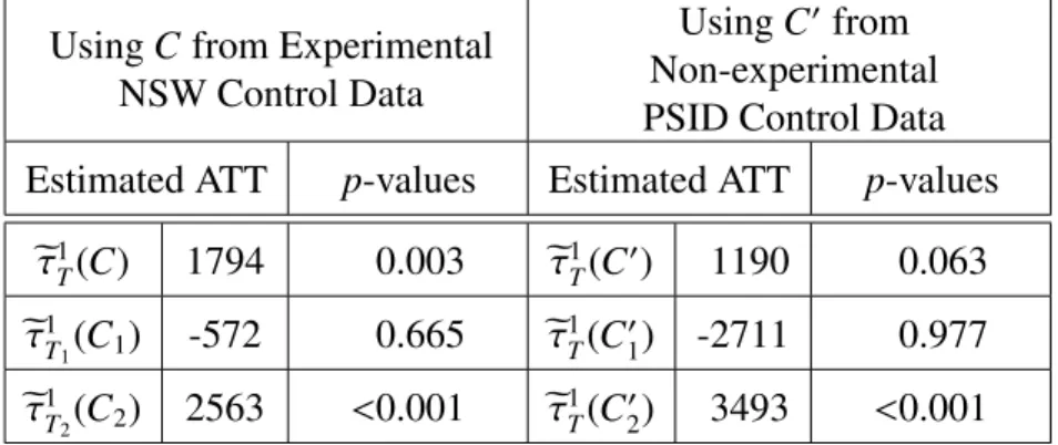
In the dissertation, the testing procedure is then applied to LaLonde (1986) data. LaLonde (1986) analyzed a dataset from National Supported Work (NSW) Demonstration program. It is a labor training program conducted in 1970s and the dataset has been used by numerous researchers. In addition to the entire sample analysis described above, a sub-sample analysis is done. The p-values obtained by entire sample analysis and sub-sample analysis obtained by Bootstrap hypothesis

(33)

tests will be provided.

The technique developed here enables to identify whether a specific subgroup has a significant treatment effect. It can be also applied to any program evalua-tion data not only restricted to this labor training program which was taken for a demonstration in my dissertation.

1.3.3 BOSS under a Multi-Treament Setting

Matching method was introduced in a binary treatment setting (Cochran and Ru-bin, 1973; RuRu-bin, 1973) and later it was extended in a multi-treatment setting (Im-bens, 2000; Lechner, 2001; Yang et al., 2016). On the other hand, so far, BOSS estimators were only applied to datasets having binary treatment with treatment indicator 0 for control units and 1 for treated units. In this section, BOSS estima-tor that is applicable to datasets having multiple treatments is proposed. As in the binary treatment setting, BOSS under a multi-treatment setting is a non-matching technique which directly minimizes an extended imbalance measure and it does not require to find a matched pair for each treated unit.

Before introducing a new BOSS estimator for multiple treatments, a matching method for the multi-treatment setting by Yang et al. (2016) is reviewed. Then a new BOSS estimator for multiple treatments is proposed and it is shown that the proposed estimator is unbiased for the expected value of the sample average treatment effect under certain conditions.

In the dissertation, a computational result demonstrating that the proposed BOSS estimator outperforms the other matching estimators in terms of the size of bias on a simulated dataset is provided.

1.3.4 Handling Missing Data in Observational Studies with BOSS

In this part of the dissertation, methods that are applicable when there is a miss-ing covariate vector or some missmiss-ing entries in the set of covariates are discussed. Both matching and BOSS relies on strong ignorability assumption as mentioned earlier. In this dissertation, a sensitivity analysis of BOSS estimators is conducted to investigate how the estimated values change when the conditional independence (unconfoundedness) assumption is violated because of a missing covariate vector. To conduct a sensitivity analysis, a number of hidden/unmeasured covariate

(34)

vec-tors were generated based on some parameter values using the method proposed and implemented by Ichino et al. (2008) and Nannicini (2007). How this addition affects the BOSS estimates and its standard error compared to matching estimates are investigated.

In addition, two different BOSS methods that are applicable after multiple im-putation on a dataset with missing entries in covariates are compared. Mitra and Reiter (2016) studied two propensity score matching methods (namely, Across and Within approaches) and showed that Across approach leads to a smaller bias than Within approach. Across approach estimates the propensity score, averages the propensity scores from the multiple datasets whose missing values are im-puted, and finds a single treatment effect estimate. On the other hand, Within ap-proach conducts the propensity score matching to find a treatment effect estimate on each imputed dataset and finds a mean of the estimates. Similar approaches in estimation using BOSS are defined and examined. The performance of two BOSS methods are compared to each other as well as to the corresponding methods in matching.

1.3.5 Duality in BOSS

Last part of the dissertation studies a dual problem of the BOSS formulation. As stated earlier, BOSS can be formulated as an MIP. The integer constraints in the MIP can be relaxed and the BOSS can be formulated as an LP if a fractional contribution of control units in the optimal control group is allowed. Accordingly, a dual problem of the LP can be found. Since understanding the meaning of the variables and constraints in the dual problem is important, it is investigated as a last part of the dissertation.

1.3.6 Outline

This dissertation is organized in the order that is mentioned above: Chapter 2 dis-cusses on bias in Balance Optimization Subset Selection, Chapter 3 disdis-cusses on treatment effect decomposition and bootstrap hypothesis testing in observational studies, Chapter 4 discusses on BOSS under a multi-treatment setting, Chapter 5 discusses on handling missing data with BOSS, Chapter 6 discusses on duality in BOSS, and Chapter 7 concludes.

(35)

CHAPTER 2 BIAS IN BALANCE OPTIMIZATION

SUBSET SELECTION

2.1 Introduction

The Balance Optimization Subset Selection (BOSS) framework was proposed by Nikolaev et al. (2013) as an alternative to matching methods for causal inference using observational data. Due to advances in computing technology, this opti-mization approach using Mixed Integer Programming (MIP) was enabled. This approach directly minimizes an imbalance measure while traditional matching methods do so indirectly.

Recently, Zubizarreta (2012) formulated a matching method as an MIP with a term directly minimizing imbalance which differs from traditional matching meth-ods. The formulation for BOSS is similar to this matching method as an MIP but it differs in that BOSS does not require each treatment unit to be matched with a control unit.

BOSS finds a control group that is more balanced (i.e., a control group that is more similar to the treatment group in its covariate value distribution) than those identified by traditional matching methods because BOSS directly minimizes a given imbalance measure. In this chapter, selection bias is defined as the diff er-ence in mean control response of the treatment units and that of the selected con-trol units. Within the BOSS framework, eliminating this bias as much as possible is one of the aims of this chapter.

There have been numerous papers that have studied bias in causal analysis. Unlike randomized experiments which select treated and control units at random, bias from systematic differences in these two different groups of units is inevitable in observational studies. Rubin (1973) viewed matching as a way of removing and controlling the bias. Rosenbaum and Rubin (1985) explored the bias which arises from incomplete matching. Heckman et al. (1998) characterized the selection bias by decomposing it. They tested assumptions for matching methods and showed

(36)

which component of the bias is associated with matching. Abadie and Imbens (2012) introduced matching estimators that are bias-corrected.

As stated, bias associated with the matching estimator has been studied by many researchers. However, a study of the bias in the treatment effect estimator based on the BOSS framework is also necessary. What causes bias in BOSS and how to reduce it are considered in this chapter.

When using Balance Optimization Subset Selection, bias in the treatment ef-fect estimator occurs as a result of the following cases. First, it can occur when an incorrect imbalance measure that does not comply with a functional form of the response function is used. Second, even with a correct imbalance measure, bias can be generated when there are insufficient data leading to residual imbal-ance between the outcome groups. Non-zero bias can also result when an optimal value of zero cannot be found because of technical issues like ineffective algo-rithms and time constraints. It is called suboptimality in this chapter. Examples corresponding to each of these cases generating bias will be provided.

The chapter is organized as follows. Section 2.2 investigates the relationship between bias and the imbalance measure used by BOSS. Section 2.3 defines the concept of the Balance Hierarchy and discusses how to identify the correct imbal-ance measure. Section 2.4 provides examples illustrating the relationship between bias and imbalance measures. Section 2.5 further studies the cases where residual balance remains after optimization due to insufficient data and/or suboptimality from technical issues. Section 2.6 combines the requirements to guarantee zero bias from the BOSS estimator. Section 2.7 provides concluding comments.

2.2 Relationship between Bias and Imbalance

Measure

2.2.1 Role of Covariate Balance for Reducing Bias in the

Treatment E

ff

ect Estimator

This section studies the relationship between bias and an imbalance measure. Ex-amples illustrating this relationship is provided in this section and Section 2.4. Before going on to the examples, first recall that the sample average treatment effect for the treated (SATT) is defined as (1.3).

(37)

Further recall that the treated and untreated responses for unituare of the forms

Yu1 = h1(Xu)+u1 and Yu1 = h0(Xu) +u0 for a treatment response function h1(·)

and a control response functionh0(·). Then the difference between the estimated treatment effect,_eτ1_T(C0), and the SATT,τ1_T, as the sum of selection bias and the error terms can be written as follows.

eτ 1 T(C 0 )−τ1_T =        1 |T| X t∈T Y_t1− 1 |C0_| X c∈C0 Y_c0        −        1 |T| X t∈T Y_t1−Y_t0        =        1 |T| X t∈T Yt0− 1 |C0_| X c∈C0 Yc0        =        1 |T| X t∈T h0(Xt)− 1 |C0_| X c∈C0 h0(Xc)        | {z } B(T,C0_{) : selection bias} +         1 |T| X t∈|T| 0 t − 1 |C0_| X c∈C0 0 c         | {z } E(T,C0_{): error terms} (2.1) Here it is assumed that the error term0

u for any unitu is zero in expectation.

Hence, in expectation, the difference of the estimated treatment effect and the SATT,_eτ1

T(C 0

)−τ1

T, is reduced to the selection bias,B(T,C 0

), which is defined as the control response function mean of the treatment units minus that of the control units.

On the response functions h0(Xu) and h1(Xu), the BOSS framework does not

have any specific requirements other than those required for unbiasedness based on imbalance measures. These two response functions need not be the same. Heterogeneity in the effects for treatment and control units will be identified after conducting BOSS from a non-zero treatment effect estimate.

In the special case where the treatment response function is the same as the control response function, the following relationship between the estimated ATT and selection bias holds. Under this case that h0₍_X

u) = h1(Xu), the SATT, τ1T, is

zero in expectation. Accordingly, the expected value of the estimated treatment effect is the same as the expected value of selection bias. That is,

E h eτ 1 T(C 0 )i= E        1 |T| X t∈T Yt1− 1 |C0_| X c∈C0 Yc0       

(38)

= E        1 |T| X t∈T h1(Xt)− 1 |C0_| X c∈C0 h0(Xc)       +E        1 |T| X t∈T 1 t − 1 |C0_| X c∈C0 0 c        (2.2) = E        1 |T| X t∈T h0(Xt)− 1 |C0_| X c∈C0 h0(Xc)        = EB(T,C0)

In BOSS, the objective function of the optimization problem is defined as some measure of covariate imbalance. A non-zero objective value, in general, leads to non-zero bias. However, zero bias may be obtained even though there is residual imbalance in the full joint distribution. Examples 1 and 2 illustrate those possibil-ities.

Example 1. Consider the three covariate case with the untreated response function

h0₍_X

u) = 1.4Xu,1 + 1.3Xu,2 + 0.9Xu,3 for both treatment and control individuals. Then the bias is defined by

B(T,C0)≡ P t∈Th0(Xt) |T| − P c∈C0h0(X_c) |C0_| . (2.3)

Given the linear response function, B(T,C0)= P t∈T(1.4Xt,1+1.3Xt,2+0.9Xt,3) |T| − P c∈C0(1.4Xc,₁+1.3Xc,₂+0.9Xc,₃) |C0_| =1.4(XT,1−XC0_,₂)+1.3(XT_,₂−XC0_,₁)+0.9(XT_,₃−XC0_,₃), (2.4) whereXG,k =Pu∈GXu,k/|G|forG∈ {T,C0}.

Under some generic form for the response function, it is common to have both non-zero objective value and non-zero bias. To illustrate this case of non-zero objective with a particular objective function as defined in (2.6), it is necessary to introduce some additional notation.

Let P = {1,2,3} be the set of covariate indices. Denote the set of values that the k-th covariate can have by Nk and suppose that the possible values for each covariate are 1 and 2: Nk ={1,2}fork∈ P. LetEk,jdenote the bin of units whose k-th covariate is equal to j, i.e., Ek,j is the set of units that have the value j for

theirk-th covariate wherek ∈ P, and letηk,j(G) ≡ |Ek,j∩G|forG ∈ {T,C0}. For

(39)

with j= 2 is for covariate value 2. Assume that the distributions of the treatment groupT and the selected control groupC0 satisfy the following:

η1,1(T)=100, η1,2(T)= 50, η2,1(T)=50, η2,2(T)= 100, η3,1(T)=75, η3,2(T)= 75, η1,1(C0)=100, η1,2(C0)= 50, η2,1(C0)=48, η2,2(C0)= 102, η3,1(C 0 )=76, η3,2(C 0 )= 74. (2.5)

For a subset of covariate indices, K ⊂ P, use the objective function from Sauppe et al. (2014) p.551: IK(T,C0)= X k∈K X j∈Nk |ηk,j(T)−ηk,j(C 0 )| (2.6)

Here K = P = {1,2,3}. The objective value that is computed based on (2.6) is given by 0+0+2+2+1+1=6 and the bias is given byB(T,C0)=−17/1500 since

XT,1 = XC0_,₁= (100+2·50)/150,XT_,₂ =(50+2·100)/150,XC0_,₂ =(48+2·102)/150,

XT,3 =(75+2·75)/150, andXC0_,₃ = (76+2·74)/150.

Example 2. Note that sometimes zero bias may be obtained even in the case when the objective value is not zero. To illustrate, consider an example with the same ηk,j as above but with a different response function h0(Xu) = 1.4Xu,1+1.3Xu,2 + 2.6Xu,3. In this case, a zero-bias is obtained although the objective function is non-zero.

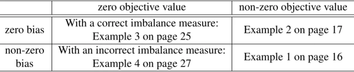
The relationship between the bias and the objective function value after opti-mization is summarized in Table 2.1. All four scenarios can happen as indicated. Example 3 and 4 corresponding to zero-objective value will be introduced later in Section 2.4.1.

Table 2.1: Relationship between objective function value and the bias zero objective value non-zero objective value zero bias With a correct imbalance measure:

Example 3 on page 25 Example 2 on page 17 non-zero

bias

With an incorrect imbalance measure:

(40)

Sauppe and Jacobson (2017) shows that covariate balance can be used to guar-antee unbiasedness of treatment effect estimates under certain assumptions on the control response function which relates the covariates to the control responses. The required imbalance measures for several different functional forms of the con-trol response function are summarized below.

LetK denote a subset of the set of all the covariate indices P= {1,2,· · · ,K}. If the response function has a term of the form P

k∈KβkXu,k for a unitu, then an

imbalance measure that includes the following term is needed: IDOM:K(T,C0)= X k∈K 1 |T| X t∈T Xt,k− 1 |C0_| X c∈C0 Xc,k . (2.7)

If the response function has a term of the formγKQk∈K(Xu,k)pk for some

con-stants pk ∈ _R fork ∈ K and γK ∈ R, then an imbalance measure that includes

the difference in corresponding correlation terms as in the following equation is needed: ICorr:K(T,C0)= X k∈K 1 |T| X t∈T Y k∈K (Xt,k)pk− 1 |C0_| X c∈C0 Y k∈K (Xc,k)pk . (2.8) When a response function isseparable for each covariate, an imbalance mea-sure that balances the marginal distribution of those covariates such as IKS or ICvM, which will be discussed in Section 2.3.1, will be needed. (Definition of a separable response function and a non-separable response function will be ex-plained in page 21.)

2.3 Balance Hierarchy and Correct Imbalance

Measure

In this section, correct and incorrect imbalance measures will be defined. First, a concept of balance hierarchy is introduced.

Definition 1. An imbalance measureI1is said to have ahigher rank in the bal-ance hierarchythan an imbalance measureI2ifI1 = 0 impliesI2= 0. In other words,I1 is more highly ranked thanI2ifI1requires more balance thanI2.

Consider the following imbalance measures including the ones used in the pre-vious examples.

(41)

For covariatesk=1,2,· · · ,K, • Difference of Means: IDOM(T,C0)= K X k=1 1 |T| X t∈T Xt,k− 1 |C0_| X c∈C0 Xc,k (2.9)

• Difference of First and Second Moments: IDOM+DOV(T,C0)=IDOM+

K X k=1 1 |T| X t∈T Xt,k 2 − 1 |C0_| X c∈C0 Xc,k 2 (2.10) • Bivariate Moment:

IDOM2(T,C0)=IDOM₊DOV+

X (k1,k2)∈(P₂) 1 |T| X t∈T Xt,k1Xt,k2 − 1 |C0_| X c∈C0 Xc,k1Xc,k2 (2.11) whereP₂denotes a set of all the possible covariate index pairs.

• Kolmogorov-Smirnov Test Statistic: IKS(T,C0)= K X k=1 max x∈Xk(T∪C0) Fkb(T,x)−Fkb(C 0_, x) (2.12)

where Xk(S) ≡ {Xu,k : u ∈ S} denotes the set of possible values for

thek-th covariate value for all unitsu∈S, andFkb(T,x) is the empirical

distribution function of the treatment groupT while Fkb(C0,x) is that of

the control group C0_{. That is,} b Fk(T,x) = u∈T : Xu,k ≤ x /|T| and b Fk(C0,x)= u∈C0 : Xu,k ≤ x /|C 0 |. • Joint Distribution: Iecdf:D(T,C 0 )=X D∈D max x∈XD(T∪C0) FDb (T,x)−FDb (C 0_, x) (2.13)

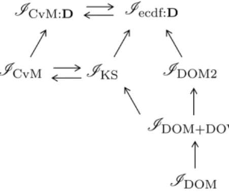
where Ddenotes the set of all possible covariate clusters. A covariate cluster denotes a set of covariate indices and thusDis the power set of P={1,2,· · · ,K}.

(42)

According to Definition 1, the imbalance measure IDOM₊DOV is more highly ranked in the balance hierarchy than the imbalance measureIDOMbecause it re-quires more balance between the matched groups to achieve zero objective value when using this imbalance measure as an objective. Similarly, IDOM2 is more highly ranked than both IDOM and IDOM₊DOV. As additional terms to be bal-anced are included, the corresponding imbalance measure will be ranked higher and higher.

In addition, IKS is more highly ranked in the balance hierarchy than both im-balance measures IDOM₊DOV and IDOM since IKS requires the entire marginal distribution of the covariates to be balanced while the others only require a bal-ance in first and second moments.

In that sense, the imbalance measureIecdf:Din (2.13) would be among the most

highly ranked imbalance measures since it requires a balance in joint distributions while the other measures such asIDOM, IDOM₊DOV, andIKS require balance on marginal distributions only and IDOM2 balances bivariate moments only among the many other possible combinations of clusters for balancing.

Note that some ranks of imbalance measures are not comparable. For example, there does not exist a strict ranking between a middle ranked imbalance mea-sure and an imbalance meamea-sure created by combining a low ranked imbalance measure with a high ranked imbalance measure. Additionally, among the above examples, the rank of IDOM2 and IKS cannot be compared since IDOM2 has a correlation term thatIKS does not balance while the former does not balance the entire marginal distribution as the latter does.

Figure 2.1: Balance Hierarchy Example

The ranks of the above imbalance measures are summarized in Figure 2.1. The arrow indicates a direction from a low ranked imbalance measure to a high ranked imbalance measure. If there does not exist a directed path from one imbalance

New developments in causal inference using balance optimization subset selection

ABSTRACT

ACKNOWLEDGMENTS

TABLE OF CONTENTS

TABLES

FIGURES

ABBREVIATIONS

NOTATION

CHAPTER 1

INTRODUCTION

1.1

Introduction

1.2

Background on Balance Optimization Subset

Selection Framework

1.2.1

Randomized Experiments and Observational Data

1.2.2

Matching

1.2.3

Balance Optimization Subset Selection (BOSS)

1.2.4

Comparison between Genetic Matching and BOSS

1.3

Overview

1.3.1

Bias in BOSS

1.3.2

Treatment E

ff

ect Decomposition and Bootstrap Hypothesis

Testing in BOSS

1.3.3

BOSS under a Multi-Treament Setting

1.3.4

Handling Missing Data in Observational Studies with BOSS

1.3.5

Duality in BOSS

1.3.6

Outline

CHAPTER 2

BIAS IN BALANCE OPTIMIZATION

SUBSET SELECTION

2.1

Introduction

2.2

Relationship between Bias and Imbalance

Measure

2.2.1

Role of Covariate Balance for Reducing Bias in the

Treatment E

ff

ect Estimator

2.3

Balance Hierarchy and Correct Imbalance

Measure