generating a stochastic graph
Emmanuel Gobet, Gustaw Matulewicz
To cite this version:
Emmanuel Gobet, Gustaw Matulewicz. Parameter estimation of Ornstein-Uhlenbeck process generating a stochastic graph. 2016. <hal-01271994>
HAL Id: hal-01271994
https://hal-polytechnique.archives-ouvertes.fr/hal-01271994
Submitted on 9 Feb 2016
HAL is a multi-disciplinary open access archive for the deposit and dissemination of sci-entific research documents, whether they are pub-lished or not. The documents may come from teaching and research institutions in France or abroad, or from public or private research centers.
L’archive ouverte pluridisciplinaire HAL, est destin´ee au d´epˆot et `a la diffusion de documents scientifiques de niveau recherche, publi´es ou non, ´emanant des ´etablissements d’enseignement et de recherche fran¸cais ou ´etrangers, des laboratoires publics ou priv´es.
Parameter estimation of Ornstein-Uhlenbeck process
generating a stochastic graph
Emmanuel Gobet∗, Gustaw Matulewicz†
February 9, 2016
Abstract
Given Y a graph process defined by an incomplete information observation of a multivariate Ornstein-Uhlenbeck process X, we investigate whether we can estimate the parameters ofX. We define two statistics ofY. We prove convergence properties and show how these can be used for parameter inference. Finally, numerical tests illustrate our results and indicate possible extensions and applications.
Keywords: stochastic graph process, inference for stochastic process, incomplete information, asymptotic properties of estimators.
MSC 2010: 62Mxx; 05C80; 62F12.
1
Introduction
1.1 Statement of the problem
Take an Ornstein-Uhlenbeck process X = (Xt : t ≥ 0) with values in Rd (d ∈ N+), solution to the stochastic differential equation:
dXt=−AXtdt+ ΣdWt, X0 given. (1.1)
We consider the model of stochastic graphs generated as follows: the adjacency value between verticesiand j is
Ytij =1Xt∈Sij
where Siji,j are subsets ofRd.
The topic of random graphs is a well-developed research area. Since the Erd˝os–R´enyi model, many other ways of generating a random graph have been proposed, most notably the preferential attachment model, the Chung-Lu model or the Kronecker graph model [Bol01,MX07]. Most models have the goal to create a single instance of a random graph.
∗
CMAP, Ecole Polytechnique and CNRS, Universit´e Paris Saclay, Route de Saclay, 91128 Palaiseau cedex, France. Email: [email protected].
†
CMAP, Ecole Polytechnique and CNRS, Universit´e Paris Saclay, Route de Saclay, 91128 Palaiseau cedex, France. Email: [email protected]. This work was funded jointly by Chaire Risques Financiersof theRisk Fondation, theFinance for Energy Market Research Centreand the Natixis Foundation for Quantitative Research.
Some proceed by ”growing” the graph, i.e. by successively adding nodes and edges, as in the preferential attachment model. Other models also enable deleting nodes and edges.
In contrast, in our model the nodes are fixed, hence it is not a ”growing” graph, but the edges are evolving continuously in time. One could in principle fix aT and consider the random graph YT, but the real richness of our model resides in the evolution of the graph in continuous time. For instance, it adds correlation between graphs at arbitrary time-scales.
Y gives only partial information aboutX. Hence, usual results on inference for stochas-tic processes can not be applied. We therefore aim at extending these results to our setting and ask then the question of findingA,Σ from Equation (1.1), given the sole observation ofY.
We will consider that we have access to one realization of the process Y observed at discrete times (k∆n)0≤k≤n,n≥1. Therefore, we hope to get results in the long time limit
n∆n→+∞asn→+∞, in which we can expect to use ergodic properties of the process
X. Intuitively, doing so we will estimate parameters arising in the stationary distribution. Also, to estimate parameters related to local fluctuations (i.e. Σ), we are interested in the high frequency limit ∆n→0.
1.2 Applications in systemic risk modeling
In [CFS15,FI13], authors present a model for inter-bank lending in whichdbank reserves are modeled through real-valued random processesXi. Whenever bankihas more reserves than bankj, ilends money to j, thus reducing reserve Xi and increasing Xj. Gaussian noise is added in order to model random variations of the reserves. We will refer to this model through Equation (1.2) (which is exactly the model from [CFS15] without a central bank): dXti =−a d d X j=1 Xti−Xtj dt+σdWti. (1.2)
In this model, authors define a systemic event when the mean reserve falls below some predetermined value. The analysis of the model shows that the probability of the systemic event can be computed and the result depends explicitly on the values of the parameters, especially on the correlation of the Brownian motions with a common noise.
Therefore, it is crucial to know how to estimate the values of the parameters of the equation, even in the realistic situation where one wouldn’t have complete information of the banks’ reserves. We consider for instance that the regulator, whose perspective we are analysing here, would fix a regulatory threshold r and would observe all variables of the form Ytij :=1Xi t−X j t>r. 1.3 Summary of results
• An ”occupation time” statistic OTn, which counts the number of times the process is present in a given set. Normalized by n, this number converges to the stationary measure of that set, in the following ways:
– inL2, with a speed of convergence bounded by√n∆n, which is the square root of the time horizon of the estimation;
– with the right normalization, convergence in law to a Gaussian variable, for one-dimensional processes.
• A ”crossings” statistic Cn, which counts the number of times the process X goes in or out of a given set Sij, i.e. the number of changes of the Yi,j-value. We show a convergence in L2 of this - suitably normalized - statistic.
We show then how to use this in order to estimate the parameters of model (1.1).
1.4 Related work
The question that we investigate in this article is on the recovery of the parameters of an Ornstein-Uhlenbeck equation given thenobservations of a single realization of the process. It relates therefore to the largely developed field of inference for stochastic processes. Many results exist on this subject: for instance, see [Kut04] for continuous-time observations and [KLS12] for discrete-time ones.
In this work, we are specifically interested in discrete-time observation schemes. We observe three distinct discrete-time settings. First, the low-frequency long-time (LF-LT) setting consists in fixing a time step ∆ and observing at times (i∆)i≤n with n → +∞ [Yos92]. Second, the high-frequency fixed-time (HF-FT) setting, where a time horizon T
is fixed and observations are taken at (i∆n)i≤n with ∆n = T /n → 0 [GJ93]. Third, the high-frequency long-time (HF-LT) setting where one assumes observations at (i∆n)i≤n with the time step ∆n → 0 and the time horizon n∆n → +∞ [Kes97, Gob02, ASM04]. Our work is placed in the latter HF-LT setting.
Some results already exist on problems with observation of crossings of a given thresh-old. For instance, [Flo87] considers the estimation using only the observation of the sign of the process. However this is done in the LF-LT setting and in dimension 1. The same remark applies to [Flo89,Flo91]. We will extend her CLT results to the HF limit.
The HF-LT setting is combined with partial information observation in [IUY09]. The authors consider, for > 0, the observation of 1|Xt|≥Xt. Our assumption of a binary
observation leaves us with even scarcer information, thus making the inference problem more delicate.
To sum up, the closest work to ours is seemingly [IUY09] and [Flo87] but our main orig-inal contribution concerns the multi-dimensional scope and the case of binary observation in the HF-LT setting.
Organisation of the paper. In the next subsection, we define the notations and assumptions used throughout this work. Then in Section 2, we study the first statistic based on occupation time. We first prove general convergence results useful to analyse the convergence of all estimators (Theorem 2.1). L2 and CLT results are proved (Theorems
(Theorem 3.1). Last in Section 4, we report numerical experiments. Applications to parameters inference are discussed along the sections. Technical results are postponed to Appendix.
1.5 Notations and assumptions 1.5.1 Notations
For d ∈ N+, take m ∈ Rd and V a symmetric positive definite d×d matrix. We call
N(m, V) the law of a Gaussian r.v. with mean m and covariance matrix V. Form = 0, this centered Gaussian distribution is denoted byνV and its density byµV:
µV(x) = (2π)−d/2det(V)−1/2exp −1 2x ∗V−1x , x∈Rd,
wherex∗ is the transpose ofx. In dimensiond= 1, we introduce additionally the CDF of
N(0,1):
N(x) =
Z x
−∞
µ1(s)ds, x∈R.
Given a measurable function f : Rd → R and a probability measure ν on Rd, we denote ν(f) = R
f(x)ν(dx). For a measurable set S ⊂Rd, we write ν(S) = ν(1
S) by a slight abuse of notation.
1.5.2 Restatement of the model and standing assumptions
Consider two matricesA ∈ Md,d(R) and Σ∈ Md,q(R) where d, q ∈N+, which serves to model (1.1). The standing assumptions onA and Σ are the following.
(H) The matrix ΣΣ∗ is invertible and the spectrum of A has strictly positive real parts:
a0 := min
λ∈Sp(A)
Re(λ)>0. (1.3)
We define an important class of covariance matrices:
Vt= Z t 0 e−AuΣΣ∗e−A∗udu, V∞= Z +∞ 0 e−AuΣΣ∗e−A∗udu.
We easily check thatV∞ is well defined, symmetric positive definite. For one-dimensional processes, we simply have:
vt= σ2 2a 1−e −2at , v∞= σ2 2a. Let Ω,F,(Ft)t∈R+,P
be a filtered space and (Wt)t∈R+ a q-dimensional Brownian motion with respect to F. In this setting, we consider the multi-dimensional Ornstein-Uhlenbeck equation forX as introduced in (1.1):
dXt=−AXt+ ΣdWt, X0 d
where X0 is a r.v. independent of W. In the following X = (Xt : t ≥0) stands for the Rd-valued solution of (1.4). We recall some properties from [KS91, Chapter 5.6]. First X is stationary:
∀t∈R+, Xt
d
=N (0, V∞). (1.5) To simplify we denote byν∞ the Gaussian distributionN (0, V∞) and by µ∞ its density. In the subsequent analysis, the initial distribution could be different from ν∞, it would not change significantly the analysis since the OU-process converges exponentially fast to its stationary regime.
Second,X is Markovian and ergodic. Take t > s, we can write:
Xt=e−A(t−s)Xs+
Z t s
e−A(t−u)ΣdWu, (1.6)
from which we deduce
Xt|Xs
d
=N e−A(t−s)Xs, Vt−s
. (1.7) Equality (1.6) gives also an important insight on decorrelation of the process:
Cov (Xt, Xs) =e−A(t−s)Var (Xs) =e−A(t−s)V∞, t≥s. (1.8) In the following, all the limits will be considered asn→+∞, under the asymptotics of high frequency data (∆n→0) on a long-time interval (n∆n→+∞). Also, for simplicity, we assume ∆n≤1.
Remark 1.1. In Equations(1.4)and(1.7), we see that the distribution ofX0 andXt|Xs depend on Σ only through ΣΣ∗. Hence we shall restate our inference problem as the estimation of(A,ΣΣ∗).
2
Occupation time statistic
Consider thed-dimensional process governed by Equation (1.4). We define the first statis-tic:
Definition 2.1. Let S be a measurable subset of Rd. Define:
YtS=1Xt∈S.
The occupation time statistic is defined as:
OTSn= 1 n n−1 X k=0 YkS∆n = 1 n n−1 X k=0 1Xk∆n∈S.
2.1 Preliminary tools
The study of convergence of OTSn and further statistics will be made possible by using some tight controls related to the mixing properties ofX at different times. Note that we cannot directly invoke general mixing properties of Markov chains since here the Markov chain (Xk∆n :k ≥0) depends on nthrough ∆n: this is the main difficulty. The current estimates are made possible using the Gebelein inequality (a.k.a. Lancaster inequality) about maximal correlation between Gaussian spaces.
Theorem 2.1 (Mixing properties). Assume that X solves the Ornstein-Uhlenbeck Equa-tion (1.4), and recall the definition of a0 in (1.3). There exists a finite constant C(2.1),
depending only on the stationary distribution covariance matrix V∞, such that for any
t≥s≥0 and for any functions ϕ:C0([0, s],Rd)→R, φ:C0([t,+∞),Rd)→R such that
ϕ, φare square-integrable w.r.t. the law of X, we have
|Cov (ϕ((Xu)u≤s), φ((Xv)v≥t))| ≤C(2.1)e−a0|t−s|
q
Var (ϕ((Xu)u≤s))Var (φ((Xv)v≥t)). (2.1) The proof is done in AppendixB. A very useful corollary is related to the convergence study of sum of general local functionals ofX.
Corollary 2.1. Consider a measurable function g:N×N× C0([0,1],Rd)→R such that E
g(k, n,(Xs)k∆n≤s≤(k+1)∆n)
2
<+∞ for any k, n∈N. For n∈N define
v2n= sup k<nV ar g(k, n,(Xs)k∆n≤s≤(k+1)∆n) , ξk(n)= r ∆n n g(k, n,(Xs)k∆n≤s≤(k+1)∆n).
Then, there is a finite constantC(2.2), dependent only on the parametersA,Σof the model,
such that: Var n−1 X k=0 ξ(kn) ! ≤C(2.2)v2n. (2.2) Remark 2.1. If E h Pn−1 k=0ξ (n) k i
→l for some l∈R, then vn→0 implies
n−1
X
k=0
ξk(n) −→L2 l.
Proof of Corollary2.1. Denote gk = g(k, n,(Xs)k∆n≤s≤(k+1)∆n); without loss of
general-ity, we can assume thatE[gk] = 0. We have
Var n−1 X k=0 ξ(kn) ! = ∆n n n−1 X k=0 Var (gk) + 2∆n n n−1 X k=0 n−1 X l=k+1 Cov (gk, gl).
For l > k, we have [k∆n,(k+ 1)∆n]⊂ [0,(k+ 1)∆n] and [l∆n,(l+ 1)∆n] ⊂[l∆n,+∞[. Apply Theorem2.1:
Cov (gk, gl)≤C(2.1)e−a0|k+1−l|∆n
p
Then we deduce Var n−1 X k=0 ξk(n) ! ≤ ∆n n nv 2 n+ 2∆n n n X m≥0 C(2.1)vn2e−a0m∆n ≤vn2 ∆n+ 2C(2.1) ∆n 1−e−a0∆n ≤C(2.2)v2n,
where we set C(2.2) = supx∈[0,1]
x+ 2C(2.1)1−ex−a0x
.
2.2 L2 convergence of occupation time statistics
Theorem 2.2. For any measurable set S ⊂Rd, OTS
n converges toν∞(S) in L2 and E(OTSn−ν∞(S))2 =O 1 n∆n .
Proof. As the process is stationary, EOTSn = E[1X0∈S] = ν∞(S). Next, we apply Corollary2.1to OTSn =Pn−1 k=0ξ (n) k with ξk(n) = 1 n1Xk∆n∈S= r ∆n n g(k, n, Xk∆n), g(k, n, Xk∆n) = 1 √ n∆n1 Xk∆n∈S, Var (g(k, n, Xk∆n)) = 1 n∆nV ar 1Xk∆n∈S = ν∞(S) (1−ν∞(S)) n∆n .
Therefore, we getE(OTSn−ν∞(S))2
=Var OTSn≤ C(2.2) n∆n .
2.3 Central Limit Theorem for one-dimensional processes
Here we restrict the study to the one-dimensional situation. There are two technical reasons for this: we solve explicitly the Poisson equation (see Lemma C.2) and derive tractable bounds on it. Additionally, we take advantage of the one-dimensional situation to handle explicit computations. The validity of a Central Limit Theorem in the multi-dimensional setting remains an open question to us.
Ford= 1, the model becomes
dXt=−aXtdt+σdWt. (2.3)
Assumption (H) readsa >0 andσ 6= 0. We consider the caseS= [1,+∞[. The extension of the following results to the case whereS is a finite union of intervals is straightforward, and it is left to the reader.
Theorem 2.3. As n→+∞, we have p n∆n OT[1n,+∞[−ν∞([1,+∞[) d − → N 0, ν∞ σ2F02
where F is defined in (C.2) and is such that
F0(x) = 2 σ2 N√x∧1 v∞ −N√1 v∞ N√x v∞ µ∞(x) ∈ 0,2 r π aσ2 .
Proof. A simple inspection onF0 shows that it is non-negative. The upper bound is proved in LemmaC.3(see inequality (C.7)). This proves the inclusion ofF0(x).
We now prove the Central Limit Theorem. We follow the approach by [Flo84]. The main difference is that the function x 7→ 1x≥1 is non continuous, which raises technical
issues.
Consider first the continuous time extension of OT[1n,+∞[, i.e.
OTct = 1
t
Z t
0
1Xs≥1ds.
Denote in this prooff(x) =1x≥1 and ˆf(x) =f(x)−ν∞([1,+∞[), so that
Z t
0
ˆ
f(Xs)ds=t(OTtc−ν∞([1,+∞[)).
Introduce then L = −ax∂ ∂x +
σ2
2
∂2
∂x2 the infinitesimal generator of X: Lemma C.2 in AppendixCensures thatF defined in (C.2) verifies the Poisson equation
LF =−f .ˆ
IntroduceMt=F(Xt)−F(X0) +
Rt
0fˆ(Xs)ds. F is twice differentiable butF
00has a single point of discontinuity at 1. However, we can still apply Itˆo’s formula in that case (see LemmaC.1). We get: Mt= Z t 0 σF0(Xs)dWs, hMit= Z t 0 σ2F0(Xs)2ds.
F0 being bounded, M is a martingale. As we have t−1hMit →ν∞ σ2F02 in probability (ergodic theorem) as t → +∞, we can use a CLT for martingales (see Lemma C.4 with
Kt=t−1/2) to get M√t t = F(Xt)−F(X0) + (OTct−ν∞([1,+∞[))t √ t d − → N 0, ν∞ σ2F02.
Finally, F is sublinear (F0 bounded), thus √1
t(F(Xt)−F(X0)) L2 −→ 0. Consequently we have proved √ t(OTct−ν∞([1,+∞[))−→ Nd 0, ν∞ σ2F02.
We now aim at proving that the above result extends to the discrete version OT[1n,+∞[. For this, define
Dn:= p n∆n OT[1n,+∞[−OTcn∆n = r ∆n n n−1 X k=0 Z ∆n 0 f(Xk∆n)−f(Xk∆n+u) ∆n du := r ∆n n n−1 X k=0 g(k, n,(Xs)k∆n≤s≤(k+1)∆n).
Observe that it remains to prove thatDn−→P 0. In view of Corollary2.1 and since E
g(k, n,(Xs)k∆n≤s≤(k+1)∆n)
= 0,
it is enough to prove that
vn2 := sup k<n E g(k, n,(Xs)k∆n≤s≤(k+1)∆n) 2 →0.
Actually, by Jensen inequality, the stationarity property and sincef takes values in{0,1}, we have vn2 ≤ 1 ∆n Z ∆n 0 E |f(X0)−f(Xu)|2 du= Z 1 0 E [|f(X0)−f(Xt∆n)|] dt.
With probability 1,f(Xt∆n) → f(X0), sincef is continuous except on a set of zeroν∞
-measure: by the dominated convergence theorem, we obtainvn→0, thenDn−→P 0. From this we have: p n∆n OT[1n,+∞[−ν∞([1,+∞[) d −→ N 0, ν∞ σ2F02 .
2.4 Application to parameter inference Lemma 2.1. Fix S ⊂Rd and recall (H). Then ν
∞(S) is a continuous function of V∞. Proof. Write ν∞(S) = Z S µ∞(x)dx= Z S (2π)−d/2det(V∞)−1/2exp −1 2x ∗V−1 ∞ x dx.
As the determinant and the inverse are continuous functions,µ∞(x) is continuous inV∞ for any x. We also have:
µ∞(x)≤(2π)−d/2vm−d/2exp −
v−M1
2 |x|
2
!
Applying the Hoffman-Wielandt theorem ([HJ86, Theorem 6.3.5]) we know that vM and vm are continuous functions ofV∞, which are also non-zero in the neighborhood of invertible V∞. From this follows that there is a local bound (in the neighbourhood of every invertibleV∞) by an integrable function of the form:
µ∞(x)≤Cst exp −Cst|x|2
with a positive constant Cst. Conclude using the dominated convergence theorem.
For one-dimensional processes. We consider here Equation (2.3). The limit value of OTn depends on the stationary distribution of the process, which is a centered Gaussian r.v. with variancev∞=σ2/2a(see Section1.5). Ifν∞(S) is monotonous with respect to
v∞, then we can construct an estimator ofv∞.
For instance, ifS = [1,+∞[, thenν∞(S) =N −1/
√
v∞ which is strictly increasing withv∞.
However,v∞ is not a one-to-one function of aand σ hence we need more information to find the parameters of the process, using for instance the crossings statistic of Section
3.
For multi-dimensional processes. Here again the limit value of OTSn is the measure of S under the stationary distribution. This distribution depends on the value of the matrixV∞. Without further information or assumptions,V∞is a symmetricd×dmatrix, representingd(d+ 1)/2 unknowns. We can expect to be able to find these unknowns only if we consider more than one setS and the corresponding statistics.
In the following, we will use the fact that the covariance matrices of the marginals of a Gaussian variable are the restrictions of its covariance matrix to the relevant spaces.
Consider first for i≤dthe setSi ={x :xi ≥1}. Then ν∞ Si
depends only on the value of (V∞)ii. Applying the result from the preceding paragraph, we can construct an estimator of that value.
Consider then for i6= j the set Sij = {x : xi ≥1, xj ≥ 1}. Then ν∞ Sij depends only on the values of (V∞)ii,(V∞)jj,(V∞)ij. From the previous point, we know we can construct estimators of (V∞)ii,(V∞)jj. For the last parameter, we use the following result. Proposition 2.1. Take(G1, G2)a non-degenerate centered Gaussian vector. Denoteρthe
correlation betweenG1andG2. DenoteS= [1,+∞[2 andµρthe density of the distribution of (G1, G2). Then µρ(S) is a strictly increasing function ofρ.
Proof. Denoteσ1 =
p
Var (G1),σ2 =
p
Var (G2). By symmetry between G1 and G2, we
can safely assumeσ1 ≥σ2. Introduce a standard centered Gaussian G. We can write
(G1, G2)=d ρσ1 σ2 G2+σ1 p 1−ρ2G, G 2 , µρ(S) =E 1G2≥1E 1ρσ1 σ2G2+σ1 √ 1−ρ2G≥1|G2 = Z R 1y≥1N ρσ1σ2y−1 σ1 p 1−ρ2 ! µσ2 2(y)dy.
Setg(ρ, y) = ρ σ1 σ2y−1 σ1√1−ρ2: then dg dρ(ρ, y) = σ1 σ2y−ρ
σ1(1−ρ2)3/2.This is strictly positive for y≥1 since σ1
σ2 ≥ 1 and ρ < 1. Therefore N(g(ρ, y)) is strictly increasing in ρ, and so is µρ(S) on ]−1,1[.
This shows that we can construct an estimator of (V∞)ij given the knowledge of (V∞)ii,(V∞)jj, which we have as noted before. Therefore,using d(d+ 1)/2 estimators, we can recover the whole matrixV∞.
3
Crossings statistic
Given a binary observation Yt, a function of Xt, we will count how many times Y goes from 0 to 1 and vice-versa. The following defines a statistic counting the number of jumps between 0 and 1 of the discretization ofY.
Definition 3.1. We define the crossings statistic by:
CS n = 1 n n−1 X k=0 1YS k∆n6=Y S (k+1)∆n .
In the following, we restrict the convergence analysis to sets which are half-spaces
Si={x:xi ≥1}; by symmetry, we assume that i= 1. Therefore we drop the superscript
S and
Yt=1X1
t≥1.
Cn counts the number of times the discretised projection of X on the first coordinate crosses 1.
3.1 L2 convergence
Theorem 3.1. Assume that n∆3n/2 →+∞. We have the following convergence:
Cn √ ∆n L2 −→2 s (ΣΣ∗)11 2π µV∞11(1), Var C n √ ∆n =O 1 n∆3n/2 ! .
Proof. For ease of writing, introduce a new notation:
Zk(n)=1X1
k∆n<11X
1
(k+1)∆n≥1.
Now, divide the sum in two similar parts:
Cn=Cn+−+Cn−+, Cn+− = 1 n n−1 X k=0 1X1 k∆n≥11X 1 (k+1)∆n<1 , Cn−+ = 1 n n−1 X k=0 Zk(n).
Although the two sums aren’t perfectly symmetric, we will show that our reasoning will apply to both sums. Concentrate then on the second sum. In order to apply Corollary
2.1, we introduce the following notations:
C−+ n √ ∆n := n−1 X k=0 ξk(n), ξk(n)= 1 n√∆n Zk(n):= r ∆n n g k, n,(Xs)k∆n≤s≤(k+1)∆n , vn2 := sup k<n Vargk, n,(Xs)k∆n≤s≤(k+1)∆n . We obviously havevn2 = n∆12 nsupk<nVar
Zk(n)and CorollaryA.1we haveVarZk(n)=
O √∆n
. Therefore vn2 =O 1
n∆3n/2
=o(1) by assumption. Thus, Corollary2.1gives us the convergence to 0 of the variance.
Using again CorollaryA.1we get
E C−+ n √ ∆n = E h Zk(n)i √ ∆n ∼ s (ΣΣ∗)11 2π µV∞11(1). Therefore, recalling Remark2.1 gives
C−+ n √ ∆n L2 −→ s (ΣΣ∗)11 2π µV∞11(1). The same reasoning would apply toC+−
n if only we replacedZ (n) k by ˜Z (n) k =1X1 k∆n≥11X 1 (k+1)∆n<1 . Observe E h ˜ Z∆n i =E h 1−1X1 0<1 1−1X∆1n≥1 i = 1−Eh1X1 0<1 i −Eh1X1 ∆n≥1 i +E[Z∆n] =E[Z∆n]
using stationarity. Thus, we can transfer the estimate on Zk(n) to ˜Zk(n), i.e. on C−+
n to
C+−
n , which gives the final result.
3.2 Application to parameter inference
For one-dimensional processes. For d= 1, Theorem3.1 simplifies to
Cn √ ∆n L2 −→ √2σ 2πµ∞(1).
Thus the renormalizedCnconverges to a value that depends on σ and the densityµ∞(1), which itself depends onv∞=σ2/2a. In Section2.4, we show how to estimate the value of
v∞. Using this estimate, we can computeµ∞(1) and construct simply an estimator of σ. Finally, as we estimate both σ and µ∞, we also estimate a. Therefore, the two statistics OTn and Cn are sufficient to estimate the parameters of the model (2.3).
For multi-dimensional processes. As we show above, we can estimate parameters of one-dimensional processes. The extension to multi-dimensional processes is not obvious. However, in specific cases, we can leverage Theorem3.1. Consider specifically thatA is a diagonal matrix with diagonal terms (a1, . . . , ad). Then
(V∞)ij = Z +∞ 0 e−aiu(ΣΣ∗)ije−ajudu= (ΣΣ ∗)ij ai+aj .
Assuming we knowV∞, which we can estimate using results from Section 2.4, and as we can estimate (ΣΣ∗)iiusing Theorem 3.1, we can estimate the values ofai:
ai =
(ΣΣ∗)ii 2 (V∞)ii
.
We complete the inference by using the relation (ΣΣ∗)ij = (ai+aj) (V∞)ij.
4
Numerical tests
In the following, we present some inference results in the case of one-dimensional Ornstein-Uhlenbeck process. The observations are obtained via simulation and we consider simu-lation lengths nbetween 10 and 10·214 and discretization time-steps ∆ between 0.1 and 0.1·2−7.
We simulate trajectories usingσ =a= 1:
dXt=−Xtdt+ dWt.
For each data point characterized by (n,∆), we compute the expectation and standard deviation of OTn and Cn. These are empirically computed using 50000 simulated trajec-tories, independently initialized in the stationary distribution. Each figure will show these values plotted against eithernor ∆ in blue, and regression lines are added to each series in red. The figures are plotted in log-log scale, in order to show dependence of the results as powers ofnand ∆.
For some plots, the regressions don’t give a clear answer on the power dependence. Because we know many of our results come from the long-time limit, we privilege data series that maximizen∆n, the horizon of the simulation.
Plots. For programming and plotting purposes, it is clearer to define statistics OTnand
Cn omitting normalization. Therefore, only in this paragraph, we use
] OTn= n−1 X k=0 1Xk∆n>1, fCn= n−1 X k=0 1Xk∆n6=X(k+1)∆n.
Additionally, we usetsas a notation for ∆n.
Figures 1 and 2 show a linear dependence in n and no dependence in ∆. This is in agreement with the stationarity of the process.
The lines fitted to the scatter in Figure3 are somewhat misleading. Their slopes vary from from 0.52 to 0.75. However, given our analysis in the paper, it is n∆, the inferring
Figure 1: Expectation ofOT]n versusn for different values of time steps ∆n(ts)
Figure 2: Expectation of OT]n versus ∆n (ts) for different values of n
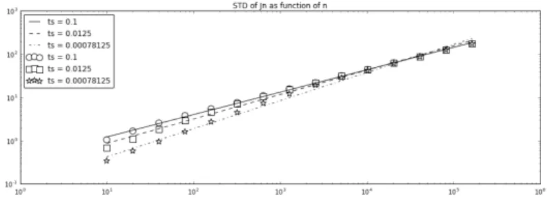
Figure 3: Standard deviation of OT]n versusn for different values of time steps ∆n (ts)
Figure 5: Expectation ofCfn versusn for different values of time steps ∆n(ts)
Figure 6: Expectation of fCn versus ∆n (ts) for different values of n
Figure 7: Standard deviation of fCn versusn for different values of time steps ∆n (ts)
horizon, that has the largest impact on the quality of the convergence. For this reason, we should concentrate on high values ofn. Further work on the last 5 points of the scatters concludes with a consistent slope of 0.5. The same applies to Figure4: although slopes vary from −0.07 to −0.5, we have the most confidence in the line corresponding to the highest value ofn. We retain then the value of−0.5.
Thus, we numerically observe (up to constants)
EhOT]n i ∼n, r VarOT]n ∼n1/2∆−1/2.
RegardingCfn, Figures5and6show clear power dependencies of 1 and 0.5 with respect
ton and ∆. Again, Figures7 and 8 have to be observed only at the largest values of n. We conclude with slopes of 0.5 and 0.
E h f Cn i ∼n∆1/2, r Var f Cn ∼n1/2.
Summary. Taking the results from the preceding paragraph and rewriting them using our regular expressions of OTn and Cn, as in Definitions 2.1 and 3.1, we get from these numerical tests:
• For OTn:
– E[OTn]∝1,
– Var (OTn)∝ n∆1n.
This is in agreement with Theorem2.2.
• For Cn: – E[Cn]∝∆1n/2, – Var√Cn ∆n ∝ 1 n∆n.
The expectation estimate is in agreement with Theorem 3.1. However, our variance estimate is seemingly not optimal: the missing factor ∆1n/2 may come from sub-tle cancellations in small time, in conjonction with the low regularity of indicator function. This issue is left to future research.
In Table1 we can compare our theoretical limits with the estimates from simulation.
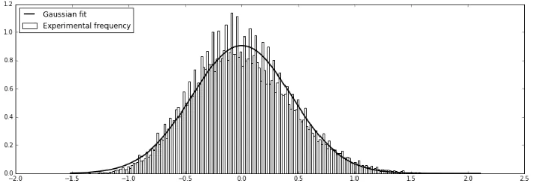
Numerical investigation regarding a central limit theorem for Cn. Our experi-mental observation ofVar Cn √ ∆n ∝ n∆1
n suggests we may expect a central limit theorem
for √n∆n Cn √ ∆n −m where m = limn→+∞E h Cn ∆n i
. However, this result is out of the scope of the present paper.
Nonetheless we use the results of our simulations in order to see whether this conjecture is likely. In Figure9, we compare the normalized histogram ofCnto the probability density function of a fitted Gaussian. The agreement of the two seems to show that the validity of a central limit theorem is likely.
Simulation result Theoretical value E[OTn] 0.07977 0.07865 Eh√Cn ∆n i 0.16418 0.16560 n∆nVar (OTn) 0.25902 N/A n∆nVar Cn √ ∆n 0.43324 N/A
Table 1: Observed versus theoretical values of the limits of the expressions on the left
Figure 9: Normalized histogram ofCn, forn= 10·214and ∆n= 0.1·2−7 and plot of PDF of Gaussian fit
A
Expectation of threshold crossing for OU processes in
small time
In this section, X is the d-dimensional Ornstein-Uhlenbeck process of Equation (1.4). Define the indicator of the crossing of the threshold 1 by the first coordinate ofX:
Z∆=1X1
0<11X1∆≥1.
From Section1.5.2, the first coordinate ofX∆|X0is a Gaussian vector centered at e−A∆X0
1
with varianceV∆11. ThereforeEh1X1
∆≥1 |X0 i =N (e−A∆X0)1−1 √ V11 ∆ and E[Z∆] = Z Rd1x 1<1N e−A∆x1−1 q V11 ∆ µ∞(x)dx. (A.1)
Lemma A.1. Let h be a boundedcontinuous increasing non-negative function, integrable in −∞ and define: Ih(∆) := Z Rd1x 1<1h e−A∆x1 −1 q V∆11 µ∞(x)dx. Then when∆→0, Ih(∆)∼ √ ∆ q (ΣΣ∗)11µV11 ∞(1) Z 0 −∞ h(x)dx.
Proof. We use the following change of variables: (y1, y2, . . . yd) = x1−1 q V∆11 , x2, . . . xd , Ih(∆) q V∆11 = Z Rd1y 1<0h e−A∆ 11 y1+ e −A∆11 −1 +P i≥2 e −A∆1i yi q V∆11 ×µ∞ 1 + q V11 ∆ y1, y2, . . . , yd dy. (A.2)
Using the power expansion of the matrix exponentiale−A∆= Id−∆A+O ∆2
, we have:
e−A∆11
= 1 +O(∆),
e−A∆1i = ∆A1i+O ∆2, i≥2.
Simultaneously, we know that V∆ ∼ ∆ (ΣΣ∗) as ∆ → 0. Hence in the integral (A.2),
h(. . .) andµ∞(. . .) converge pointwise toh(y1) andµ∞(1, y2, . . . , y2) respectively, for any
y. To pass to the limit for (A.2), it remains to dominate h(. . .)µ∞(. . .) uniformly in ∆, by an integrable function onRd.
• On the one hand, using the monotone and non-negative properties of h, we observe that h(. . .) is bounded by h(12y1+ 2P
j≥2|yj|) for anyysuch thaty1<0, provided
that ∆ is small enough.
• On the other hand, sinceV∞−1 is symmetric definite positive,µ∞(. . .) is bounded by Cst exp(−P
j≥2|yj|2/Cst) for some positive constant Cst.
Finally, we easily check that the product of the two bounds is integrable, using in particular thathis integrable onR−and bounded overR. Thus the dominated convergence theorem yields Ih(∆) q V11 ∆ → Z 0 −∞ Z Rd−1 h(y1)µ∞(1, y2, . . . yd)dy, Ih(∆)∼ √ ∆ q (ΣΣ∗)11Z 0 −∞ h(x)dx Z Rd−1 µ∞(1, y2, . . . yd)dy.
We can simply rewrite the last integral. LetG=d N(0, V∞):
Z x −∞ Z Rd−1 µ∞(y1, z)dy1dz=PG1≤x= Z x −∞ µV11 ∞(y 1)dy1
where we have used thatG1 d=N 0, V∞11
at the second equality. It gives, for any x∈R,
Z
Rd−1
µ∞(x, y2, . . . yd)dy=µV11 ∞(x), and therefore the announced result.
Corollary A.1. In the limit ∆→0, we have E[Z∆]∼Var (Z∆)∼ √ ∆ s (ΣΣ∗)11 2π µV∞11(1).
Proof. Since Z∆ takes values in {0,1}, if E[Z∆] → 0, we have Var (Z∆) = E[Z∆] (1−
E[Z∆])∼E[Z∆]. Thus, it remains to show the estimate on E[Z∆].
Start from (A.1) and apply Lemma A.1 with h(·) =N(·). We have R−∞0 N(x) dx =
1
√
2π, hence the result.
B
Maximal correlation inequality
In this section, we aim at proving the very useful Theorem2.1.
B.1 Gebelein’s inequality We start by an abstract version.
Theorem B.1([Jan97, Theorem 10.11]). TakeH,K two closed subspaces of some Gaus-sian Hilbert space. DefinePHK the restriction to H of the orthogonal projection onto K. Define the maximal correlation coefficient between variables A, B respectively measurable w.r.t. the sigma field generated byH and K:
ρ(H, K) = sup
A∈L2(H),B∈L2(K)
|Cor (A, B)|.
Then we have:
ρ(H, K) =kPHKk where k · k is the operator norm.
We now restate in a more convenient way the above result in a finite dimensional case and for given Gaussian vectors: we believe such a statement may exist in the literature but we could not find a ready reference. Consider a Gaussian Hilbert space and two Gaussian vectors X, Y in this space. Define then HX and HY the subspaces spanned respectively byX andY.
Denoting PXY the orthogonal projection on HY restricted toHX, from TheoremB.1 we have thatρ(HX, HY) = kPXYk. This value is independent of the enclosing Gaussian Hilbert Space.
Using the notations stated above, set
ρ(X, Y) =ρ(HX, HY) =kPXYk.
Corollary B.1. Take X,Y two Gaussian vectors in the same Gaussian Hilbert space and
f, g two functions such that f(X),g(Y) are square-integrable. Then we have:
|Cov (f(X), g(Y))| ≤ |ρ(X, Y)|pVar (f(X))Var (g(Y)).
In preparation of Theorem 2.1, we now aim at making more explicit the coefficients
B.2 Finite-dimensional Gaussian vectors
Notation. We denoteCov (X) the covariance matrix ofXandCov (X, Y) the covariance matrix of X and Y, which is also the upper-right part of the covariance matrix of the vector (X, Y). We reserve the notation Var (X) for the variance of a real-valued
X.
We setKXX =Cov (X),KY Y =Cov (Y) andKXY =Cov (X, Y). AsKXX andKY Y are symmetricnon-negative definite matrices, there existOX, OY orthogonal matrices and
DX, DY diagonal non-negative definite matrices such that we have:
KXX =OX∗DXOX = O∗XDX1/2OX O∗XD 1/2 X OX ∗ , KY Y =OY∗DYOY = O∗YDY1/2OY O∗YD 1/2 Y OY ∗ . Note thatO∗XDX1/2OX andO∗YDY1/2OY are symmetric.
Take now X0 and Y0 orthonormal basis of respectively HX and HY. It is easy to see that the covariance matrixR of X0 and Y0 is the projection matrix from HX on HY written in the basisX0 and Y0 and therefore ρ(X, Y) =kRk.
B.2.1 Non-degenerate case
Assume, in this paragraph, DX and DY are non-degenerate or, equivalently, that KXX andKY Y are non-degenerate.
We can chooseX0 = OX∗ DX1/2OX −1 XandY0 = OY∗D1Y/2OY −1 Y. Our calculation shows then that
R =OX∗D1X/2OX −1 KXY OY∗D1Y/2OY −1 .
From the other side,O∗XD1X/2OX andOY∗D1Y/2OY are symmetric matrices which square toKXX and KY Y. Therefore we have
(KXX)1/2 =O∗XD
1/2
X OX, (KY Y)
1/2
=O∗YDY1/2OY. From this we have the following proposition.
Proposition B.1. Take (X, Y) a Gaussian vector. Assume that Cov (X), Cov (Y) are non-degenerate. Then we have
ρ(X, Y) =kCov (X)−1/2Cov (X, Y)Cov (Y)−1/2k.
Corollary B.2. IfX andY are orthogonal with non degenerate components (Var Xi
6
= 0, Var Yj6= 0, for anyi, j), then we have ρ(X, Y) =kRk with
Rij =Cor Xi, Yj
= Cov X i, Yj p
B.2.2 Degenerate case
In this part, we consider that X or Y is degenerate (or both). We know there are or-thonormal matricesOX andOY such thatOXXandOYY both have diagonal covariances. These diagonals can have zero values; taking only the variables of OXX and OYY that have non-zero variances, we get a couple of orthonormal families. Applying results from previous paragraph and using the fact that extending a matrix with zeroes doesn’t change its operator norm, we have the following.
Proposition B.2. Let (X, Y) be a Gaussian vector andOX,OY two orthogonal matrices such that XO := OXX and YO := OYY are respectively orthogonal families. Then the maximal correlation coefficient verifies ρ(X, Y) =kRk with
Rij =CorXOi , YOj= Cov(Xi O,Y j O) q Var(Xi O)Var(Y j O) if Var XOi VarYOj6= 0, 0 if Var XOiVar YOj = 0.
B.3 Application to functions of Gaussian processes
We are now in a position to give the maximal correlation betweenXsandXtfort, s∈R+, in terms of the OU parameters (A, Σ) (Assumption (H)).
Proposition B.3. Using the previous notation, we have for anys, t∈R+
ρ(Xs, Xt)≤
r
vM
vm
e−a0|t−s|,
where a0 := minλ∈Sp(A)Re(λ), vM = maxλ∈Sp(V∞)λ, vm= minλ∈Sp(V∞)λ.
Proof. Lett≥s≥0. From (1.5) and (1.8), we have
Cov (Xs) =Cov (Xt) =V∞, Cov (Xt, Xs) =e−A(t−s)V∞.
SinceV∞ is non degenerate (owing to Assumption(H)), we can apply propositionB.1, to get
ρ(Xs, Xt) =kV∞−1/2e−A(t−s)V∞1/2k.
The bound onρ(Xs, Xt) is a consequence of sub-multiplicativity of the operator norm. We immediately deduce the following.
Corollary B.3. For any ϕ, φ:Rd→R square-integrable w.r.t. ν∞, we have
|Cov (ϕ(Xs), φ(Xt))| ≤
r
vM
vm
e−a0|t−s|pVar (ϕ(Xs))Var (φ(Xt)).
We can proceed to the proof of Theorem2.1. In its setting we havet > s ≥0 and ϕ,
Proof. For ease of writing, denote ϕs =ϕ (Xu)0≤u≤s and φt =φ (Xv)v≥t . Without loss of generality, we can assume E[ϕs] = E[φt] = 0.We repeatedly use the Markov property and the tower property of conditional expectation to write
Cov (ϕs, φt) =E[ϕsφt] =E[ϕsE[φt| Fs]] =E[ϕsE[φt|Xs]] =E[E[ϕs|Xs]E[φt|Xs]] =E[E[E[ϕs|Xs]φt|Xs]] =E[E[ϕs|Xs]φt] =E[E[ϕs|Xs]E[φt|Xt]] =Cov (E[ϕs|Xs],E[φt|Xt]).
We define nowf(Xs) =E[ϕs|Xs], g(Xt) =E[φt|Xt] and apply Corollary B.3:
Cov (f(Xs), g(Xt))≤
r
vM
vm
e−a0|t−s|pVar (f(Xs))Var (g(Xt)).
Then, the announced inequality of Theorem 2.1 stems from the standard decomposition Var (h) =Var (E[h| G]) +E[Var (h| G)]≥Var (E[h| G]) for any sigma-field G and any square-integrable variableh.
C
Central limit theorem for discontinuous functions of OU
processes
In this section, we broaden the domain of application of the properties from [Flo84], precisely extending it to the case of a bounded function with a single point of irregularity, asx7→1x≥1. In this section, the processX is one-dimensional.
C.1 Itˆo formula for piecewise C2 function
First, we recall a generalization of Itˆo’s lemma to functions that are not C2.
Lemma C.1. Let g be a function g : R → R, twice differentiable and g00 is continuous except at a single point z. Assume also that ∀x 6= z,|g00(x)| ≤ K. Then Itˆo’s formula applies to g, i.e.: dg(Xt) =g0(Xt)dXt+ σ2 2 g 00(X t)dt.
Proof. As we have g ∈ C1 and g00 is integrable on any interval, we can apply [RW87, Lemma 45.9].
C.2 Solution to Poisson equation LF =−f
Consider now a functionf smooth with the exception of a single point. Consider also L
the infinitesimal generator associated toX verifying (2.3):
Lφ(x) =−ax∂φ ∂x(x) + σ2 2 ∂2φ ∂x2(x).
The next lemma gives a solution to the Poisson equationLF =−f. Lemma C.2. Let f be a bounded function. Then
F(x) :=− 2 σ2 Z x 0 dy µ∞(y) Z y −∞ f(u)µ∞(u)du (C.1) is a solution to LF =−f. With f =1[1,+∞[−N −1/ √ v∞, we have: F(x) = 2 σ2 Z x 0 N u∧1 √ v∞ −N 1 √ v∞ N u √ v∞ µ∞(u) du. (C.2)
Proof. Simple computations give:
∂F ∂x(x) =− 2 σ2µ ∞(x) Z x −∞ f(u)µ∞(u)du, ∂2F ∂x2(x) =−2 2ax σ2µ ∞(x) Z x −∞ f(u) σ2 µ∞(u)du−2 f(x) σ2 . We then deduceLF =−f. Choosing f = 1[1,+∞[−N −1/ √ v∞ = 1−1]−∞,1[−N −1/ √ v∞ = −1]−∞,1[ + N 1/√v∞ , we get: F(x) = 2 σ2 Z x 0 dy µ∞(y) Z y∧1 −∞ µ∞(u)du− Z x 0 N√1 v∞ µ∞(y) dy Z y −∞ µ∞(u)du = 2 σ2 Z x 0 N u∧1 √ v∞ −N 1 √ v∞ N u √ v∞ µ∞(u) du.
We now establish bounds onF and its derivatives.
Lemma C.3. Assume thatf is bounded and such that ν∞(f) = 0. Define F as in (C.1). Then there exist finite constants C(C.3), C(C.4), C(C.5) (depending only on the model) such that, for any x∈R,
|F(x)| ≤C(C.3)|f|∞|x|, (C.3) |F0(x)| ≤C(C.4)|f|∞ 1∧ 1 |x| , (C.4) |F00(x)| ≤C(C.5)|f|∞. (C.5)
Proof. Using the assumption thatν∞(f) =RRf(x)µ∞(x)dx= 0, we can write: F0(x) =− 2 σ2µ∞(x) Z x −∞ f(u)µ∞(u)du = 2 σ2µ∞(x) Z +∞ x f(u)µ∞(u)du, |F0(x)| ≤ 2 σ2µ∞(x) Z x −∞ |f(u)|µ∞(u)du∧ Z +∞ x |f(u)|µ∞(u)du .
Applying now the assumption thatf is bounded, we have:
|F0(x)| ≤ 2|f|∞ σ2 N−√|x| v∞ µ∞(x) . (C.6)
Using the classic inequalityN(−|x|)≤e−x2/2 yields
|F0(x)| ≤ 2|f|∞ σ2 exp −2xv∞2 1 √ 2πv∞exp −2xv∞2 ≤2 r π aσ2|f|∞. (C.7)
By integrating, we complete the proof of Equation (C.3). Next, we use the Mills inequality,
N(−|x|)≤ e
−x2/2
√
2π|x|,
which combined with (C.6) gives
|x||F0(x)| ≤ 2|f|∞ σ2 |x| N−√|x| v∞ µ∞(x) ≤ 2|f|∞ σ2 |x| 1 √ 2π√|x| v∞ 1 √ 2πv∞ ≤ 2|f|∞ σ2 v∞.
Thus, joined with (C.7), Inequality (C.4) is proved. Last, asLF =−f,
|F00(x)|= 2 σ2 axF0(x)−f(x) ≤ 2 σ2 a2v∞ σ2 + 1 |f|∞= 4 σ2|f|∞, which proves (C.5).
C.3 CLT for multi-dimensional continuous-time martingales
Lemma C.4 ([van00, Theorem 4.1]). Let (Mt;Ft :t≥0) be ad-dimensional continuous local martingale. If there exist invertible, non-random d×d-matrices (Kt : t ≥ 0) such that ast→ ∞
• KthMitKt∗
P
−→ηη∗ where η is a randomd×d-matrix;
• |Kt| →0;
then, for eachRk-valued random vectorX defined on the same probability space asM, we have
(KtMt, X)
d
−→(ηZ, X) as t→ ∞,
References
[ASM04] Y. Ait-Sahalia and P.A. Mykland. Estimators of diffusions with randomly spaced discrete observations: A general theory. Ann. Statist., 32(5):2186–2222, 10 2004. [Bol01] B. Bollob´as. Random Graphs. Cambridge Studies in Advanced Mathematics, 2nd
edition, 2001.
[CFS15] R. Carmona, J.-P. Fouque, and L.-H. Sun. Mean field games and systemic risk. Commun. Math. Sci., 13(4):911–933, 2015.
[FI13] J.-P. Fouque and T. Ichiba. Stability in a model of interbank lending. SIAM J. Financial Math., 4(1):784–803, 2013.
[Flo84] D. Florens-Zmirou. Statistics on crossings of discretized diffusions and local time. Stochastic Processes and their Applications, 39(1):139 – 151, 1984.
[Flo87] D. Florens-Zmirou. Estimation du param`etre d’une diffusion par les changements de signe de sa discr´etis´ee. Comptes Rendus de l’Acad´emie des Sciences Paris, 305:661 – 664, 1987.
[Flo89] D. Florens-Zmirou. Approximate discrete-time schemes for statistics of diffusion processes. Statistics, 20(4):547–557, 1989.
[Flo91] D. Florens-Zmirou. Statistics on crossings of discretized diffusions and local time. Stochastic Processes and their Applications, 39(1):139 – 151, 1991.
[GJ93] V. Genon-Catalot and J. Jacod. On the estimation of the diffusion coefficient for multi-dimensional diffusion processes. Annales de l’institut Henri Poincar´e (B) Probabilit´es et Statistiques, 29(1):119–151, 1993.
[Gob02] E. Gobet. LAN property for ergodic diffusions with discrete observations.Annales de l’Institut Henri Poincare (B) Probability and Statistics, 38(5):711–737, 2002. [HJ86] R.A. Horn and C.R. Johnson, editors. Matrix Analysis. Cambridge University
Press, New York, NY, USA, 1986.
[IUY09] S.M. Iacus, M. Uchida, and N. Yoshida. Parametric estimation for partially hidden diffusion processes sampled at discrete times. Stochastic Processes and their Applications, 119(5):1580 – 1600, 2009.
[Jan97] S. Janson.Gaussian Hilbert Spaces. Cambridge Tracts in Mathematics. Cambridge University Press, 1997.
[Kes97] M. Kessler. Estimation of an ergodic diffusion from discrete observations. Scan-dinavian Journal of Statistics, 24(2):211–229, 1997.
[KLS12] M. Kessler, A. Lindner, and M. Sørensen, editors.Statistical methods for stochas-tic differential equations, volume 124 of Monographs on Statistics and Applied Probability. CRC Press, Boca Raton, FL, 2012. Revised papers from the 7th S´eminaire Europ´een de Statistique on Statistics for Stochastic Differential Equa-tions Models held in Cartagena, May 7–12, 2007.
[KS91] I. Karatzas and S.E. Shreve.Brownian Motion and Stochastic Calculus. Graduate Texts in Mathematics. Springer New York, 1991.
[Kut04] Y.A. Kutoyants. Statistical inference for ergodic diffusion processes. Springer Series in Statistics. Springer-Verlag London, Ltd., London, 2004.
[MX07] M. Mahdian and Y. Xu. Stochastic Kronecker graphs. In Anthony Bonato and Fan R. K. Chung, editors, WAW, volume 4863 of Lecture Notes in Computer Science, pages 179–186. Springer, 2007.
[RW87] L. C. G. Rogers and D. Williams. Diffusions, Markov processes and Martingales, vol 2: Ito calculus. John Wiley, 1987.
[van00] H. van Zanten. A multivariate central limit theorem for continuous local martin-gales. Statistics and Probability Letters, 50(3):229 – 235, 2000.
[Yos92] N. Yoshida. Estimation for diffusion processes from discrete observation. Journal of Multivariate Analysis, 41(2):220 – 242, 1992.
![Figure 4: Standard deviation of ] OT n versus ∆ n (ts) for different values of n](https://thumb-us.123doks.com/thumbv2/123dok_us/9486359.2823907/15.892.252.642.889.1039/figure-standard-deviation-ot-versus-ts-different-values.webp)