COMPUTATIONAL STUDY OF THE EFFECTS OF PROTRUDING STUDS CASING TREATMENT ON
THE PERFORMANCE OF AN AXIAL TRANSONIC TURBOFAN
By
MAX DAVID COLLAO
Robert S. Webster
Research Associate Professor of Computational Engineering (Chair)
Kidambi Sreenivas
Research Professor of Computational Engineering
(Committee Member)
James C. Newman III
Professor of Computational Engineering (Committee Member)
Matt Matthews
Associate Dean of the College of Arts and Sciences
COMPUTATIONAL STUDY OF THE EFFECTS OF PROTRUDING STUDS CASING TREATMENT ON
THE PERFORMANCE OF AN AXIAL TRANSONIC TURBOFAN
By
MAX DAVID COLLAO
A Dissertation Submitted to the Faculty of the University of Tennessee at Chattanooga in Partial Fulfillment of
the Requirements of the Degree of Doctor of Philosophy in Computational Engineering
The University of Tennessee at Chattanooga Chattanooga, Tennessee
Copyright © 2017 By MAX DAVID COLLAO
ABSTRACT
Turbo-compressors play a crucial role in the operation of air-breathing engines and special attention is given to the compressor’s ability to withstand adverse operating conditions. Various methods have been devised in order to enhance compressor stability and increase compressor stall margin, usually with some sacrifice of performance and efficiency. Active methods make use of external devices injecting and/or bleeding air from the compressor duct. Passive methods are primarily based on casing treatments, often involving flow paths into the rotor casing, to affect the behavior of the flow in favorable ways. In either case, it is desirable that the stability enhancing method be as simple as possible and that it keep performance and/or efficiency degradation to a minimum.
The present work consists of a CFD analysis performed to evaluate the impact of a novel form of passive stability control on the operation of an axial flow fan stage. The casing treatment consists of “studs,” which are solid structures protruding from the casing into the duct. These structures are located slightly downstream of the fan rotor trailing edge. The stage that is studied in this investigation is the NASA SDT2-R4 transonic turbofan. The simulation software used is “Tenasi,” an in-house developed flow solver.
Various simulations were conducted of the turbofan operation with and without casing treatment. Measures of performance and efficiency of the turbofan stage with no casing treatment were computed, and the results showed good agreement with available experimental data. The
computed results from simulation with casing treatment suggest that protruding studs have the potential to improve the stability of the turbofan. The computed stall margin increase using an initial configuration of protruding studs is about 5.4% in terms of mass flow rate, with a decrease in efficiency of about 1.6%. The flow-field was investigated through visualizations of flow features in order to understand the mechanisms of flow instabilities and stability enhancement. Other simulations were also carried out using modifications of the original studs to assess further changes in performance.
DEDICATION
ACKNOWLEDGEMENTS
First and foremost, I would like to thank God. Because He loved me first before I loved Him.
I am very grateful to Dr. Robert S. Webster for allowing me to work with him, for sharing his expertise in the field of turbomachinery and for serving as my adviser throughout my time doing research. I would like to thank Dr. Kidambi Sreenivas for his support and his ideas in carrying forward simulations and CFD analysis. I would like to thank Dr. James C. Newman III for serving in my committee and for serving as a leader at the SimCenter. I would like to say thanks to Dr. Matt Matthews for serving in my committee and for his great dedication as a math professor. I would also like to thank Dr. Timothy W. Swafford, Dr. Reinhold C. Mann, and Dr. Steven L. Karman Jr for their service as leaders and mentors.
Finally, I will always be thankful to my friends and family, both in the United States and in Peru. Their cheer and support was critical during my most difficult times. You all are a blessing! Thank you guys!
TABLE OF CONTENTS
ABSTRACT ... iv
DEDICATION ... vi
ACKNOWLEDGEMENTS ... vii
LIST OF TABLES ... xi
LIST OF FIGURES ... xii
CHAPTER 1. INTRODUCTION ... 1
1.1 What about compression systems? ... 1
1.2 Types of Turbo-Compressors ... 2
1.3 Instabilities in Axial Compressors ... 5
1.4 Stability Control Methods... 6
1.4.1 Active ... 6
1.4.2 Passive... 7
1.5 CFD Application to Turbo-Machinery ... 8
2. MATHEMATICAL DESCRIPTION OF THE FLOW... 9
2.1 Control Volume vs. System ... 9
2.2 Equations Describing the Fluid Flow ... 12
2.2.1 Conservation of Mass ... 12
2.2.2 Conservation of Momentum ... 13
2.2.3 Conservation of Energy ... 14
2.2.4 Thermodynamic Relations for Perfect Gas ... 15
3. COMPRESSION SYSTEM AND CASING TREATMENT ... 18 3.1 SDT2-R4 ... 18 3.1.1 Overview ... 18 3.1.2 Performance Considerations ... 20 3.1.3 Modification... 22 3.2 Protruding Studs ... 22 3.2.1 Description... 23
3.2.1.1 Elongated “U” Shape ... 23
3.2.1.2 Dome Shape... 26
3.2.2 Origin... 26
3.2.3 Search for Similar Form of Casing Treatment ... 29
4. COMPUTATIONAL PROCEDURE ... 30
4.1 Flow Solver ... 30
4.1.1 Tenasi ... 30
4.1.2 Aspects of Numerical Solution ... 31
4.1.2.1 Spatial Discretization ... 31
4.1.2.2 Temporal Discretization ... 32
4.1.2.3 Turbulence Modelling ... 33
4.1.2.4 Boundary and Initial Conditions ... 33
4.2 Mesh Generation... 34
4.2.1 General Concepts ... 34
4.2.2 Procedure ... 36
4.2.3 Detail of Interpolative Interface and Studs Volume Mesh... 40
4.2.4 Finalizing the Mesh ... 43
4.3 Setting Up and Running Cases... 44
4.4 Post-Processing and Visualization ... 46
5. RESULTS OF BASELINE SIMULATIONS ... 47
5.1 Performance Maps ... 48
5.1.1 Fan Performance ... 48
5.1.2 Stage Performance ... 51
5.2 Analysis of Flow Field ... 55
5.2.1 Location of Shocks by Operating Condition ... 55
5.2.2 Low Momentum Regions by Operating Condition ... 62
5.2.3 Instability Region in Near-Stall Operating Condition... 65
6. CASING TREATMENT SIMULATION ... 76
6.1 Performance Maps ... 77
6.1.1 Original Studs ... 77
6.1.2 Variation of Studs ... 81
6.1.2.1 Performance by Levels of Protrusion ... 82
6.1.2.2 Half Extension and Dome Shaped Studs ... 85
6.2 Flow-Field Analysis ... 87
6.2.1 Radial Distribution of Axial Flow Velocity... 87
6.2.2 Radial Distribution of Relative Flow Angles... 97
6.2.3 Flow-Field Features at 131.7 kPa Back Pressure ... 99
6.2.4 Flow-Field Features at New Near-Stall Conditions With Casing Treatment ... 105 6.2.5 Studs 1 vs. Studs 2... 109 7. CONCLUDING REMARKS ... 112 7.1 Conclusions ... 112 7.2 Recommendations ... 115 REFERENCES ... 117 VITA ... 120
LIST OF TABLES
3.1 Stage design parameters... 20 6.1 Change in performance across results for eleven tested back pressures. ... 80
LIST OF FIGURES
1.1 Various types of compressors [4] in (a) a TF30-P-6 Pratt & Whitney engine, (b) a
Lycoming T53 turboshaft engine, and (c) a Saturn MD-120 engine. ... 4
2.1 Depiction of a control volume. ... 10
2.2 Relation between systems and control volumes [1]. ... 12
3.1 SDT2-R4 installed in wind tunnel. ... 19
3.2 Experimentally measured performance curves for the SDT2-R4 stage [2]. ... 21
3.3 Full wheel of simulated stage... 22
3.4 Protruding studs S1 and S2 ... 24
3.5 Dimensions as percentage of fan chord length at tip, alignment, and location of studs. ... 25
3.6 Aft-looking-forward view of dome studs and blades... 26
3.7 Protruding rings from Lin’s work [3] (including caption from original text)... 27
3.8 Performance curve using trailing edge ring [3] ... 28
4.1 Minimum and maximum point spacing used in different regions of the turbofan stage.... 36
4.2 Surface mesh on parts of stage... 37
4.3 Plane cut of volume mesh near a corner. ... 38
4.4 Boundary conditions used on surfaces of the stage. ... 39
4.5 The two sliding interfaces used in earlier simulations are shown in pink, rotor blades and stator vanes are shown in light blue, and casing is shown in grey. ... 41
4.6 Surfaces separating the Rotor, Stator, and Studs volumes. ... 42
4.7 Aft-looking-forward view of volume mesh after generation and merging where the casing surface is shown in green, rotor blades and studs are depicted in pink, and a plane cut of the volume mesh is depicted in grey... 43
4.8 Sample of mass flow computed across four boundaries in three consecutive simula-tions... 46
5.1 Planes of integration of mass flow, total pressure and total temperature... 48
5.2 Fan total pressure ratio... 50
5.3 Fan total temperature ratio. ... 50
5.4 Fan adiabatic efficiency. ... 51
5.5 Stage total pressure ratio. ... 52
5.6 Stage adiabatic efficiency. ... 52
5.7 Temperature ratio across stage for choked flow conditions, peak efficiency, and near stall at 100% speed. ... 54
5.8 Mass imbalances at solution termination where the values are presented as a per-centage of mass flow through passage. ... 54
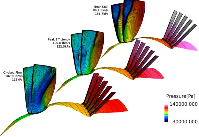
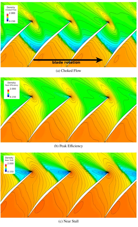
5.9 Stage surfaces colored by static pressure at different flow conditions. ... 56
5.10 Radial cut at 60% span colored by density (in kg/m3) for three back pressure conditions... 59
5.11 Radial cut at 95% span colored by density (in kg/m3) for three back pressure conditions... 60
5.12 Radial cut at 98% span colored by density (in kg/m3) for three back pressure conditions... 61
5.13 Stream lines and radial cuts of solution field colored by relative Mach number. ... 63
5.15 Forward-looking-aft view of constant x planes near low Mach number region. ... 64
5.16 Low momentum region near casing for baseline case near stall... 66
5.17 Forward-looking-aft view of parallel-to-shock plane cuts of low momentum region for baseline case near stall. ... 68
5.18 Low momentum region as exposed byνisosurface. ... 70
5.19 Tip gap flow patterns for baseline case near stall... 71
5.20 Flow pattern around stator vanes for baseline case near stall. ... 72
5.21 Comparing performance maps obtained when using a maximum of 29 viscous layers in the computational mesh. ... 74
5.22 Performance curves obtained in earlier stages of this work where a maximum of 29 viscous layers and a different surface mesh were used. ... 75
6.1 Stage total pressure ratio. ... 78
6.2 Stage total pressure ratio. ... 78
6.3 Stage total pressure ratio. ... 79
6.4 New studs tested... 82
6.5 Stage total pressure ratio. ... 83
6.6 Stage adiabatic efficiency. ... 84
6.7 Stage total temperature ratio. ... 84
6.8 Stage total pressure ratio. ... 85
6.9 Stage adiabatic efficiency. ... 86
6.10 Stage total temperature ratio. ... 86
6.11 Axial location of planes, where radial distribution samples were taken, displaying studs near the trailing edge of the rotor blades. ... 88
6.13 Radial distribution of axial velocities at 131kPa back pressure... 93 6.14 Comparison of axial momentum at a 75% fan blade span (78% outlet plane span)
radial cut at 131 kPa back pressure... 94 6.15 Radial distribution of axial velocities at baseline computed near stall conditions. ... 95 6.16 Comparison of axial momentum at a 75% fan blade span (78% outlet plane span)
radial cut at 131.7 kPa back pressure... 96 6.17 Definition of relative flow angle. ... 97 6.18 Comparison of relative flow angles at outlet plane... 98 6.19 Comparison of relative Mach number in passages between baseline and casing
treatment simulations, where the cuts are located at mid height of the studs
(97.8% span). ... 99 6.20 Isosurface ofνside view comparison... 102 6.21 Patterns of tip gap flow using casing treatment at 131.7kPa back pressure... 104 6.22 Recirculation on suction side of stator blades near casing for 131.7kPa back pressure. . 105 6.23 Forward-looking-aft view of isosurfaces ofν at near stall conditions using Studs 1
and Studs 2... 107 6.24 Patterns of tip gap flow using treatment at near stall conditions... 108 6.25 Recirculation on suction side of stator blades near casing for near stall conditions. ... 109 6.26 Comparison of total temperature coloration across Studs 1 and Studs 2, where the
radial cuts are located at mid height of the studs (97.8% span)... 110 6.27 Comparison of velocity vectors around Studs 1 and Studs 2, where the radial cuts at
mid height of the studs (97.8% span). ... 111 6.28 Flow patterns around Studs... 111
CHAPTER 1 INTRODUCTION
The work presented in this dissertation consists of a study of the performance effects caused by using studs protruding off of the casing in a turbofan stage. The study was performed using computational tools, and its main goal was that of exploring relatively simple methods for enhancing the flow stability in compression systems. The layout of the manuscript is as follows: Chapter I is an introductory overview of compression systems and the instabilities related to them. Chapter II provides a mathematical description of the fluid flow. Chapter III provides a description of the turbo-machine and the type of casing treatment under study. Chapter IV introduces the flow solver and describes the computational procedure that made up a great part of this work. Chapter V presents the validation of the CFD tools by comparing baseline simulation results with available experimental data. Chapter VI presents the results of simulating the operation of the turbo-machine at hand with the casing treatment, along with an analysis of the changes. Chapter VII gives concluding remarks and recommendations.
1.1 What about compression systems?
Gas compressors are present in diverse engineering applications that simplify and enhance the lives of people. From the most ubiquitous applications, such as refrigerators, to the most specialized ones, like power generation, there is frequently a need for pressurizing a gas in order to
later take advantage of the energy it stores or to feed combustion processes. Hence the importance of compression systems.
One application where compression systems are important is air breathing engines for aircraft propulsion. Actually, the role of a compression system in aircraft propulsion is beyond necessary but also critical. This is because in addition to playing a crucial role in thrust generation, the integrity of the entire propulsion system weighs heavily on the compressor’s ability to withstand adverse flight conditions that affect air intake negatively.
Compression systems in air breathing engines comprise a certain kind of turbo-machinery called turbo-compressors. In general, turbo-machines are rotating devices that interact with a fluid through blades attached to a shaft. More specifically, turbo-compressors absorb shaft work and transfer mechanical energy to continuously flowing air in order to raise its total enthalpy. In doing so, the air is moved through the duct of the compressor at various speeds (depending on its location and the components with which it interacts), and it behaves (its properties will change) in different ways.
Turbo-compressors possess features that make them suitable for engines if high power-to-weight ratios are required. Compared to other forms of compressors, they are able to displace large amounts of air in continuous flow. Furthermore, since they possess no reciprocating components, the problem of shaft balancing is less likely to occur, which makes turbo-compressors more reliable.
1.2 Types of Turbo-Compressors
Using a cylindrical frame of reference, a classification can be based on the direction of the main flow as projected on the meridional plane, z −r, of the turbo-machine. If the direction of
the flow remains mainly parallel to the axis of rotation, the compression system is called “axial” (Figure 1.1a). If the flow changes direction through the rotor’s flow path from the axial direction to the radial direction, the compressor is called “centrifugal” (Figure 1.1b). If the flow path of the rotor is more or less diagonal, then it is a “mixed-flow” compressor (Figure 1.1c). The type of compression system used in this work is of axial flow. Specifically, the turbo-machine used here is the transonic turbofan SDT2-R4, which will be further described in Chapter 4. Through the rest of this chapter, the focus will be placed on flow features and stability of axial compressors.
(a) Several rows in an axial flow compressor.
(b) Centrifugal flow compressor. (c) Mixed-flow comp.
Figure 1.1 Various types of compressors [4] in (a) a TF30-P-6 Pratt & Whitney engine, (b) a Lycoming T53 turboshaft engine, and (c) a Saturn MD-120 engine.
1.3 Instabilities in Axial Compressors
Unfortunately, turbo-compressors also have shortcomings. Namely, that when a compressor approaches its limits of operational stability, unsteady aerodynamic instabilities arise from within the machine. If these instabilities are not treated and are allowed to grow, they may turn into either compressor stall or compressor surge. The characteristic of compressor surge is flow reversal, while compressor stall is characterized by the formation of low-momentum flow regions (cells) that rotate at a fraction of the rotor speed and obstruct the incoming flow through the duct. Such phenomena can have detrimental effects on the rest of the components of the compressor and the propulsion system. A lot of study has been done in order to predict the onset of such instabilities. In that regard, the analytical work of authors such as Greitzer [5–8], F.K. Moore [9], and R. D. Moore [10], has served as a basis for further investigation of flow-field conditions that lead to unstable flow phenomena. Furthermore, allowing a compression system to function at an operating condition where flow instabilities have a noticeable presence has been identified as a concern for high cycle fatigue. An example of this is a more recent work by Hah [11]. Hence, various methodologies have been devised in order to preserve or regain flow-field stability [12].
Enhancing the stability of compression systems is the field of interest of this work. Stability is considered to be the ability of a compressor to recover from disturbances that take a compression system away from an operational equilibrium point [13]. In this work, stability is also considered as the ability of a compression system to withstand the turbo-compressor’s self initiated instabilities under adverse flow conditions.
Instabilities in the flow-field arise from interaction of secondary flows and other flow phenomena (e.g. passage shock) in the compressor. The secondary flow that has the most influence
in the turbo-machine used in this work is the tip leakage flow [14, 15]. This flow is driven from the pressure side to the suction side of a rotor blade by the pressure difference existing across the gap between the blade tip and the casing. The flow phenomena observed in axial flow compressors that leads to an unstable flow-field is the formation of end-wall blockage near the casing and the hub caused by boundary layer growth on these surfaces. Moreover, if the turbo-machine operates in the transonic regime, shock structures in the flow passage interact with the tip leakage flow to increase the chance for the formation of instabilities [14, 15].
1.4 Stability Control Methods
Various methods have been devised to enhance or recover stability in compressors. Based on whether or not flow is introduced into or bled off the duct flow, the stability method can be classified as passive or active.
1.4.1 Active
Active stability control on compression systems are brought by the action of devices that inject fluid into and/or bleed fluid out of the flow-field. Studies such as that by Niazi et al. [16] apply bleeding in regions of reversed flow, downstream of the rotor blades in an axial flow compressor. Their work showed that bleeding only 3% of the total mass flow enabled the extension of the operating range of the compressor. Work by Hathaway [17] shows that locating the bleeding or injection valves in strategic places of the casing can have a greater positive impact on range extension. Similar application of active devices on the flow-field of centrifugal compressors are presented by Stein et al. [18] and Skoch [19].
1.4.2 Passive
Passive methods consist of physical modifications of the components of the compressor in order to enhance stability. Therefore, there are no devices actively bleeding or injecting flow into the duct. Passive methods involve “casing treatment,” which means making geometric modifications to the casing [12].
Among the literature surveyed is the work done by Takata et al. [20] They report using five forms of casing treatment, of which two variations of skewed slots are the most successful at increasing stall margin. The mechanism introduced by these casing treatments consists of fluid from low momentum regions near the blade tip being driven upstream of the blade and into the main flow region through the slots. Similar forms of casing treatment were used by Yu et al. [21] and Emmrich et al. [22, 23]. A common finding of their work was that, due to a redistribution of the flow throughout the duct, the location where stall occurred changed from near the casing to a location near the hub. It was also observed that using the slots casing treatment delayed compressor stall until incidence angles attained large values.
Another form of casing treatment used in the experiments of Takata was circumferential grooves. Using them gave nearly the same total pressure rise as the smooth casing and had marginal impact on stall range extension. However, computational studies by Lin et al. [24, 25] show that range extension by circumferential grooves is possible when their number and location along the blade tip is chosen strategically.
The type of casing treatment used in this work is that of studs (small solid structure) protruding off the casing treatment near the trailing edge of the rotor blades. A similar form of casing treatment has not been found in the literature. However, simulations performed in this work
have shown potential for extension of the operating range. Details of the protruding studs will be provided in Chapter 4.
1.5 CFD Application to Turbo-Machinery
Computational Fluid Dynamics (CFD) has become an important tool in the study and design of turbo-machinery flow. It complements experiments by providing insight into the details of the flow that would otherwise be difficult to observe or measure using experimental methods. CFD consists of numerically solving the governing equations of fluid flow and enforcing the boundary conditions that characterize flow-fields in turbo-machinery. The present work and its findings make extensive use of CFD tools. The flow solver software used here is Tenasi, which was developed in-house. Further details about the software and the computational procedure are provided in Chapter 5.
CHAPTER 2
MATHEMATICAL DESCRIPTION OF THE FLOW
In order to solve engineering problems, it is necessary to relate fluid properties and behavior in a formal and deterministic way. The purpose here is to be able to quantify property changes, intuit the flow behavior, and predict interactions within the fluid itself and with solid bodies.
The formality of the above mentioned relations is brought by algebraic, differential and integral equations. The deterministic characteristic of these equations is achieved by deriving the relations from the laws of mechanics that apply to fluid flow. Such laws are described for a system, but in order for the equations to be useful tools in fluid dynamics analysis they are derived using the concept of control volume.
2.1 Control Volume vs. System A control volume can be imagined using Figure 2.1.
Figure 2.1 Depiction of a control volume.
A control volume is a region of space defined by surface called control surface. For the purpose of this text the control volume is labeled byΩ, and the control surface is labeled byS. If a pointBis located on the control surfaceS, a differential areadSof elemental size can be assigned toB. Also, a unit vector,n, normal to the differential areadS, and pointing outward of the control volume, is associated to dS at B, and dS = ndS can be defined. Lastly, it can be conceived that the control surface S is comprised of many of these elemental size differential areasdS, and that, similarly, the control volumeΩis comprised of many elemental size differential volumesdΩ.
A system is a defined amount of mass chosen for study. Anything outside the system is called surroundings. Dividing the system from its surroundings is the system’s boundary which
can be real or imaginary, and fixed or movable. It is through the boundary that a system interacts with its surroundings.
The use of control volumes is preferred in aerodynamics for their inherent nature of allowing mass flow through the control surface. However, since quantifying changes of the thermodynamic properties of the fluid is also very important in fluid dynamics, it is helpful to observe how control volumes and systems relate to each other. Figure 2.2, which depicts a nearly one dimensional flow
V =V(x)through a duct, is presented for that purpose. It shows at timet that the control volume between sectionsaandbis completely filled by system 2. Then, it shows that at timet+δtsystem 2 has partially moved outside of the control volume between a and b, and that the region of space abandoned by system 2 has been filled by part of system 1. In this example, the take away is that if there are flow properties changing within the control volume between a and b, some of these changes can be attributed to the moving systems carrying fluid properties.
Figure 2.2 Relation between systems and control volumes [1].
2.2 Equations Describing the Fluid Flow The governing equations are now derived from the physical laws.
2.2.1 Conservation of Mass
The conservation of mass principle states that within a system closed to any transfer of matter and energy, the amount of mass of the system remains constant over time. The meaning of this, in the context of defining a conservation of mass relation for a control volume, is that there is no such thing as a source or “sink” of mass to be taken into account. The rate of change (any variation in time) of mass inside the control volume would be attributed to the net mass flow through the control surface. This balance is shown in equation 2.1.
∂ ∂t Z Ω ρdΩ+ I S ρ(V·n)dS= 0 (2.1)
The first term on the left side of the equation is the time rate of change of the mass inside the entire control volume, whereρdΩis the mass contained in an elemental volume. In the second term,ρ(V·n)represents a mass flux (mass per unit area per unit time). Therefore, the second term represents the mass flow through the entire control surface. The conservation of mass equation is also known as the continuity equation.
2.2.2 Conservation of Momentum
The conservation of momentum law, or Newton’s second law of motion, says that the net force acting upon a body is equivalent to the body’s time rate of change of momentum. Usually this statement is presented through the vector form equalityF= ma, andFis the forceF= dP/dt
wherePis the momentum vector. For a control volume, however, the conservation of momentum principle is written as shown in equation 2.2.
∂ ∂t Z Ω ρVdΩ+ I S ρV(V·n)dS = Z Ω ρfdΩ− I S pndS+ I S (τ¯¯·n)dS (2.2)
In the first term on the left hand side, ρVdΩ represents the momentum associated with a mass in an elemental volume and the integral is the sum of the momentum throughout the entire control volume. Therefore, the first term represents the changing momentum within a control volume of an unsteady flow passing through. The second term is the sum over the entire control surface of the momentum flux, momentum carried by fluid mass passing through an elemental
surfacedS. On the right hand side, within the first term isfwhich represents body forces per unit mass in an elemental volume. Such body forces can be produced by gravity, electromagnetic fields, spin forces, or other fields that act on the volume of matter. Therefore, the first term is a volume integral of the body forces acting on the mass contained in the control volume. The second and third terms are surface integrals of forces produced by pressure and shear stresses, respectively, acting on elemental surfaces over the entire control surface. The second term has a negative sign because the forces resulting from pressure,p, point inward on the control surface. In the third term, τis the shear stress tensor.
2.2.3 Conservation of Energy
As specified for a closed system, the first law of thermodynamics states that the change of internal energy of a system is equivalent to the amount of heat transferred into the system minus the amount of work done by the system. In the case of flow through a control volume, the kinetic energy of the fluid should also be considered along with its internal energy. The conservation of energy relation for a control volume (assuming no appreciable change in potential energy) is presented in equation 2.3. ∂ ∂t Z Ω ρEdΩ+ I S ρE(V·n)dS= Z Ω ρ(f·V+q˙)dΩ− I S p(V·n)dS+ I S (τ·¯¯ V)·ndS+ I S k(∇T·n)dS (2.3) The quantityEon the left hand side is the sum of the internal energyeper unit mass and the kinetic energy|V|2/2per unit mass of the fluid within the control volume. Then, as for the previous
two conservation equations, the first term on the left hand side represents the rate of change of the total energy within the control volume; and the second term represents the net flow of total energy, where ρE(V·n)is called the energy flux.
On the right hand side, the first term accounts for both the work done by the body forces and the volumetric heating of the fluid within the control volume. The second and third terms account for the work resulting from forces acting on the surface of the control volume, pressure and shear stress, as in the momentum equation. Finally, the last term is a diffusive term that takes into account heat flux driven by temperature gradients. Fourier’s law of heat conduction is used to quantify heat flux as: FD = −k∇T, wherek is the thermal conductivity coefficient.
2.2.4 Thermodynamic Relations for Perfect Gas
In order to solve the system for all the variables necessary to define the flow, two more equations are necessary. Assuming that air behaves as a calorically perfect gas, the equation of state is used:
p= ρRT (2.4)
and the enthalpy is obtained from:
Using the following definitions:
R=cp−cv
γ = cp cv
(2.6)
The equation of state can be recast into:
p= (γ−1)ρ " E− u 2+v2+w2 2 # (2.7)
2.2.5 Complete System in Vector Form
The following is the set of governing equations written in vector form. Recasting the equations this way allows for full appreciation of all the terms involved in the system.
∂ ∂t Z Ω WdΩ+ I S (Fc−Fd)dS= Z Ω QdΩ (2.8)
The vectorW contains the conserved variables. VectorsFc andFd contain the convective
and diffusive fluxes, respectively. VectorQ contains volume sources due to heat generation and body forces. W = * . . . . . . . . . . . . . . . . . . . , ρ ρu ρv ρw ρE + / / / / / / / / / / / / / / / / / / / -(2.9)
Fc = * . . . . . . . . . . . . . . . . . . . , ρV ρuV ρvV ρwV ρHV + / / / / / / / / / / / / / / / / / / / -; V =V·n=nxu+nyv+nzw (2.10) Fd = * . . . . . . . . . . . . . . . . . . . , 0 nxτx x+nyτxy +nzτx z nxτyx+nyτy y+nzτyz nxτz x +nyτzy +nzτzz nxΘx+nyΘy +nzΘz + / / / / / / / / / / / / / / / / / / / -; Θx =uτx x+vτxy +wτx z+ k∂∂Tx
Θy = uτyx+vτy y +wτyz+k∂ y∂T
Θz =uτz x+vτzy +wτzz+ k∂∂Tz (2.11) Q= * . . . . . . . . . . . . . . . . . . . , 0 ρfx ρfy ρfz ρf·V+q˙ + / / / / / / / / / / / / / / / / / / / -(2.12)
CHAPTER 3
COMPRESSION SYSTEM AND CASING TREATMENT
In the present section, a description is given of the casing treatment and the compression system used for testing. Some insight on the origin and data available on both equipment is given. References are provided if further details are desired.
3.1 SDT2-R4 3.1.1 Overview
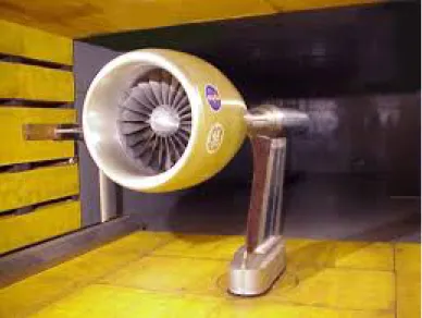
The test compression system used for the casing treatment under study is the SDT2-R4. It is an axial flow transonic turbofan stage for which a model was available and aerodynamic performance data has been published by Hughes [2]. It has previously been used at the SimCenter for validation of the in-house flow solver Tenasi, as well as for testing solver features that facilitate turbomachinery simulations [26, 27]. Other casing treatment studies have also been performed using this turbofan [24, 25]. Figure 3.1 shows the SDT2-R4 model installed at the NASA Glenn 9×5 LSWT [28].
Figure 3.1 SDT2-R4 installed in wind tunnel.
The SDT2-R4 is a 20% scale model that represesents the bypass stage of a high bypass ratio turbofan stage, representative of the technology used at the time of its creation in the early 2000’s. It was developed by General Electric Aircraft Engines (GEAE) as part of a cooperative effort with NASA on a program called “The Source Diagnostic Test” (SDT). The program had the following objectives: to establish the performance of the fan model used, the GEAE developed R4; to assess the performance of the fan when coupled with three different outlet guide vane (OGV) designs; to determine the OGV’s effect on the fan performance; and to conduct detailed acoustic and aerodynamic diagnostic surveys in order to understand the noise generation mechanisms in a turbofan engine [2]. In the SDT program, only the bypass section and not the power core section was considered [2]. Furthermore, only the Baseline OGV from the SDT program is used in the current work. Table 3.1 presents a summary of the design parameters of the SDT2-R4.
Table 3.1 Stage design parameters No. of Fan Blades 22
Fan Tip Diameter 22 in
Corrected RPM 12,657
Corrected Tip Speed 1,215 ft/sec No. of Stator Vanes 54
Corrected Weight Flow 100.5 lbm/sec-ft Stage Pressure Ratio 1.47
3.1.2 Performance Considerations
The plots in Figure 3.2 are experimental values of total pressure ratio and the adiabatic efficiency of the stage at hand. According to Hughes [2], in the experimental procedure, a Variable area Fan Exit Nozzle (VFEN) was used to obtain the performance curves below for a range of fan speed operating conditions. Through the VFEN, the exit area varied, in turn changing the back pressure on the fan to test different operating points that resembled changes in aircraft flight speed and altitude.
An important consideration from the SDT2-R4 performance curves available is that the left most points are not representative of stall conditions. It is usually the case, that the most right operating point in a performance curve represents the choking condition (where a higher mass flow through the duct is physically not possible), and that the most left operating point represents the stall condition (unstable flowfield at low mass flow rate). However, Hughes reports that the stall condition was avoided in order to avoid the risk of damaging the fan blades. When testing the fan alone, the approaching stall condition was determined by an increase in the fan blade stress being measured by blade mounted strain gauges. Furthermore, the lowest mass flow rate point tested for the entire stage was set higher than that obtained for the fan alone because, at that point, the strain
gauges had stopped working. This fact is important and will be taken into consideration later when reporting the results of the simulations.
(a) Total Pressure Ratio
(b) Adiabatic Efficiency
3.1.3 Modification
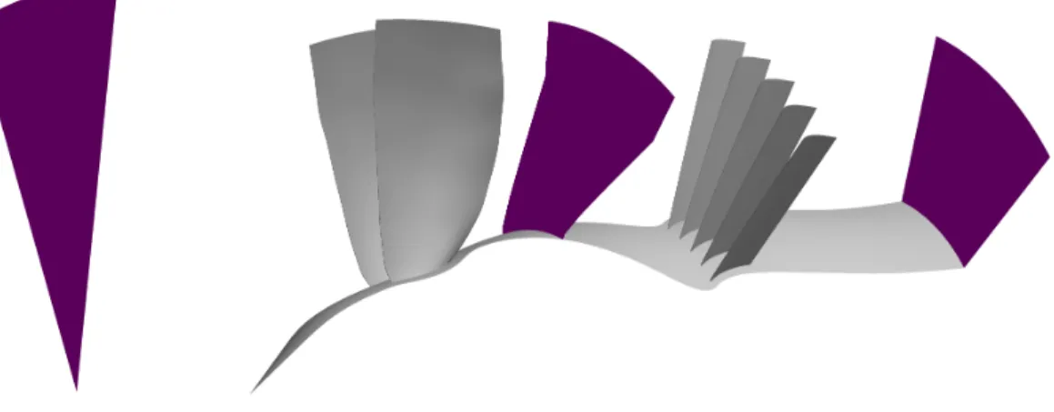
One important modification on the model of the SDT2-R4 is the addition of one stator vane. Previous computational studies have been performed on this stage with the added stator vane [26, 27], which concluded that this addition does not significantly impact the performance of the stage. The importance of adding an extra stator vane is that now the model lends itself for simulation of a one-eleventh slice of the duct (two fan blades and five stator vanes), instead of a half or the full wheel, in turn saving on computational resources while carrying out this work. Figure 3.3 depicts the full wheel of the SDT2-R4 with the added stator vane.
Figure 3.3 Full wheel of simulated stage.
3.2 Protruding Studs
The casing treatment used in this work is protruding studs. From survey of the literature, it is realized that using protruding studs has not been explored as a form of casing treatment. This
section provides a description of the protruding studs and how they came to be considered as a potential form of casing treatment.
3.2.1 Description
The studs are solid structures protruding from the casing into the duct. They are located downstream of the fan blades and in the vicinity of their tip. Two shapes of studs have been tested, elongated “U’s” and dome shaped studs. The description of each is provided next. Variation in dimensions of the “U” shaped studs were tested, while a single configuration of the dome shaped studs was simulated.
3.2.1.1 Elongated “U” Shape
The cross section in the tangential direction (with respect to the wheel) of these type of studs have the shape of a “U.” These were the first type of studs tested. The first configuration used extended in the tangential direction an angle of a fifth of a rotor pitch or approximately 3.27◦. The thickness and depth of protrusion are expressed in relation to the fan blade chord length at the tip, and they are approximately 3.2% (or 0.11in) and 4.5% (or 0.16in), respectively. Their location from the trailing edge at the tip is about 2.9% (or 0.10in). The sides of the original studs were aligned with the stagger of the fan blades at the tip. The number of these type of studs used is 55, and they are equally spaced. Because this was the first configuration of studs tested, they will be referred to by the term “S1” through the rest of this manuscript. Soon after the results of the simulations with the S1 configuration was available, a second configuration of the studs were conceived, where the sides are aligned with an angle opposite to the fan blade stagger at the tip. The second configuration of studs receives the code “S2” through the rest of the manuscript. Figure 3.4 shows the actual
models on the casing, and Figure 3.5 is a graphical description of the dimension of studs S1 and S2.
(a) From right to left: S1 and S2 (b) Aft-looking-forward view of studs and blades.
Figure 3.4 Protruding studs S1 and S2
Testing of these configurations showed an improvement in the Stall margin [29] (details in Chapter 6). Based on these results, it was decided to test variations of These designs. Variations tested included half depth studs (50% of original, H1 & H2), 125% of original(L1 & L2), and 150% of original depth (X1 & X2). Finally, the last “U” shaped type of studs to be tested were similar to the S2 studs but were to extend tangentially only 50% of the original, and twice as many of them (110) were to be used, equally spaced and in the same location with respect to the fan blades (W50).
(a) Front view: tangengial extension and depth of protrusion.
(b) Top view: width.
(c) Top view: separation from trailing edge and align-ment of sides in Studs 1.
(d) Top view: Align-ment of sides in Studs 2.
3.2.1.2 Dome Shape
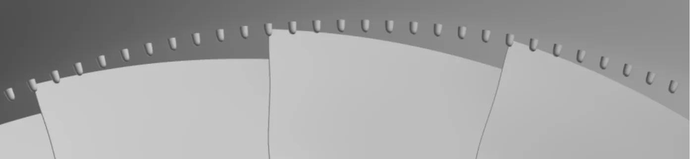
The dimensions of the studs, as with those presented in the previous section, can be manipulated in many ways, and different shapes of studs could be tested until finding a design that has the greatest positive impact on range extension without having a detrimental effect on efficiency. In order to move in that direction, one more shape of studs was explored. This stud is formed by a half revolution of the “U” shape about a vertical axis at the middle of this shape. The resulting surface of revolution resembles a dome protruding out of the casing. This type of studs receive the code “D” for the rest of this manuscript. The diameter and depth of protrusion of the D studs in terms of the fan blade chord at the tip are approximately 3.2% (or 0.11in) and 4.5% (or 0.16in). Their location behind the trailing edges of the fan blades at the tip is approximately 2.9% (or 0.10in), and there are 220 of them equally spaced across the casing. Figure 3.6 shows the domes downstream of the fan blades.
Figure 3.6 Aft-looking-forward view of dome studs and blades.
3.2.2 Origin
In his master’s thesis research, Lin worked with the same piece of turbomachinery and examined two forms of casing treatment [3]. One consisted of rings protruding into the flowfield,
located near the leading edges and the trailing edges of the fan blades. He tested three combinations of the rings: both together, a single one near the leading edge, and a single one near the trailing edge, as shown in Figure 3.7.
(a) Model showing both rings.
(b) Volume mesh with gap for trailing edge ring.
As Lin reports, the first two configurations had detrimental effects on the performance of the turbofan. Using the single one near the trailing edge, however, had an insignificant change in total pressure ratio with a small reduction in adiabatic efficiency compared to the baseline performance of the turbofan, as simulated. The performance curves from his work are shown in Figure 3.8. The idea occurred, then, to modify the ring by cutting sections from it to let some fluid through, and see what the behavior of the flow would be. Although it went undocumented, a simulation was carried out which a relative increase in range with a small decrease in efficiency. Hence the source for the idea of the, now called, protruding studs in this study. The dimensions and location of the trailing edge ring in Lin’s work were carried directly into this work.
(a) (b)
3.2.3 Search for Similar Form of Casing Treatment
After doing a survey of current literature, no report on the deliberate use of a similar type of casing treatment as the one under study here has been found. A similar effect from a stability control system was found in a piece of work by Skoch [19] where he reports the effects of introducing bleed or control tubes into the flowfield of a centrifugal compressor, from the shroud and downstream of the impeller blades in the diffuser section. An unexpected finding from his experiments was that the mere presence of the control tubes had an stabilizing effect on the flowfield without executing their function of bleeding fluid. Skoch’s report [19] reinforces the idea of possibly enhancing the stability of a flowfield by introducing structures in key regions of the duct in a compression system.
CHAPTER 4
COMPUTATIONAL PROCEDURE
4.1 Flow Solver
This section introduces the software used for performing numerical simulations and exposes some important aspects of the computations it performs. Intricacies of the numerical schemes for time and space discretizations, solutions of linear systems, stability enhancement of linear solvers, turbulence modeling, etc. are bypassed in this text since this work is focused on the stability of the operation of compression systems. References are provided as such aspects are described for when further detail is desired.
4.1.1 Tenasi
The flow solver used through the computational study reported in this manuscript is Tenasi. It has been developed at the SimCenter, at the University of Tennessee at Chattanooga, and it is used for solving a great variety of engineering problems that involve fluid flow. The range of such problems includes bronchial flows, plume dispersion modeling in urban environments, reacting flows, free surface modeling, pumps, compressors, etc.
Tenasi is a finite volume flow solver which uses an unstructured, node-centered, implicit numerical scheme. It can handle flow regimes from incompressible [30] to compressible [31]. Various options are available for turbulence modeling. Generalized interpolative interfaces and
relative frame capabilities are implemented in Tenasi [26, 27], which allow for computing flow on rotating and stationary frames interacting through a sliding interface. The solver software can run on single processor machines or on a parallel cluster of computers when solving large problems is necessary.
4.1.2 Aspects of Numerical Solution
4.1.2.1 Spatial Discretization
Representation of the space domain is carried through the use of a computational mesh. A computational mesh consists of nodes that are interconnected to form 3D cells of basic shapes. Further details on computational meshes will be provided in section 4.2.1. The flow solver Tenasi takes advantage of the mesh by using it for the spatial discretization. Control volumes are defined around the grid nodes, for which Tenasi is said to be a node-based finite-volume flow solver. The control volumes are defined by median-duals created between the mesh cells centroids. Then, the dual-faces are used as elements of the control surface for flux calculation. If the control volume, as defined in this section, is assumed not to change in time, equation 2.8 can be written as follows:
dW dt =− 1 Ω NF X m=1 (Fc−Fd)m∆Sm− (QΩ) (4.1)
In order to calculate the net flux on each control volume, the flux contributions across the faces should be established. The inviscid fluxes are approximated by solving a one dimensional approximate Riemann problem for information provided at both sides of the face, a method called the Roe scheme [32]. The viscous fluxes are approximated using the directional derivative method,
which combines information from solution gradients at the connectors (lines connecting two adja-cent points) and information available through the connectors to approximate the gradients required by the viscous terms.
4.1.2.2 Temporal Discretization
The next step is the approximation for the time derivative term in the governing equations. Equation 4.2 shows a compact recast of equation 4.1.
ΩdW
dt =−R (4.2)
The following non-linear scheme is an approximation of the time derivative [32]:
Ω∆Wn ∆t = − β 1+ωR n+1− 1− β 1+ωR n+ Ωω (1+ω)∆t∆W n−1 ; ∆Wn= Wn+1−Wn (4.3)
In the equation abovenrepresents the current time-step level. If β = 0, the time-stepping scheme is called explicit. A very basic explicit single-stage scheme is obtained by also setting ω = 0. Then, the time derivative is calculated using a forward difference, and the residual is calculated at the current time step [32].
If β , 0 in equation 4.3, the scheme is called implicit, and its advantage over a explicit scheme is increased robustness while being able to use relatively larger time steps. It is a 2nd order implicit scheme when βandω meet the condition that β = 1/2+ω[32].
4.1.2.3 Turbulence Modelling
A model is necessary to simulate turbulent flows with high Reynolds numbers. Performing a direct numerical simulation by the time-dependent governing equations is prohibitively expensive and can only be done for simpler problems at small Reynolds number values. In this work, Tenasi is set to use the one equation k − SAS turbulence model [33]. Such a model is incorporated in a “loosely-coupled” procedure, which means that the mean flow equations are first solved before solving the turbulence model independently [34].
4.1.2.4 Boundary and Initial Conditions
Boundary conditions are specified that characterize the problem as a duct flow and that truncate the physical space to a domain size that is manageable. The way they are handled is by applying the correct fluxes through the faces of the control volumes belonging to various boundaries [34]. The inflow boundary is set to desired for stagnation pressure and stagnation temperature, usually standard day total conditions. It is possible to specify the direction of the flow but not necessary. At the outflow, the value of static pressure, also called back pressure, is set to a value that will establish the conditions of the flow field between the choke point of the duct and compressor stall. The flux through both inflow and outflow boundaries is handled by a method called characteristic boundary conditions. At the solid surfaces, a adiabatic no-slip condition is enforced by applying the surface velocity on the flow and by making the velocity values at the surface nodes remain unchanged in the linear system. Axisymmetry conditions are set in the tangential direction in order to truncate the duct flow-field from a “wheel” to a “slice.” By doing this, the size of the mesh is reduced and less computational resources are necessary.
At these boundary conditions the values of the variables on one side of the slice are interpolated to the other side. Finally, generalized interpolative surfaces are established between two adjacent domains [26, 27]. This feature is useful in order to transmit variables from one domain to the other even when one domain is rotating and the other is stationary.
The initial conditions set on the flow-field for each case in this work (i.e. baseline simulation, simulation with a configuration of studs) depend on the operating condition intended to be simulated. In order to compute a set of performance curves for the stage, a first case is run with initial velocity set to zero everywhere in the duct, with the rotational speed of the rotor set to a desired value, and with the outlet boundary condition set to a static pressure that (in the simulation) will cause the duct flow to choke. Once the computed mass flow through the duct converges to a certain value, the simulation is stopped and a new case is run. A new case is set up with a higher value of static pressure at the outlet boundary and the solutions from the case previously run (i.e. velocity, density, pressure.). Once, the simulation results show mass flow convergence, the simulation is stopped for the given back pressure and the process is repeated until the entire performance curve has been computed.
4.2 Mesh Generation 4.2.1 General Concepts
The flow-field and the solid surfaces that interact with the fluid are represented using points, also called nodes. It is at these points that the variables to be solved are stored, rates of changes are determined, volume and surface integrals of sources are evaluated, and convective and diffusive fluxes between points are calculated. A computational mesh or grid is created by interconnecting
the points through connectors (or edges). Cells are formed with such connectors, which are shaped as triangles and quadrilaterals on surfaces, and tetrahedra, pyramids, prisms, and hexahedra in space. This process of subdividing the physical space through cells of basic shapes is called discretization of the space. The type of mesh used for discretization in this work is unstructured because indexing of the nodes follows no particular scheme, and a mix of different cell shapes is used.
Generation of a computational mesh is the first step in carrying out a simulation. As mentioned above, it is the way in which the flow-field for simulation is represented. Arguably, the mesh generation phase is also the most time consuming. Although, there exist simulation software packages with automatic mesh generation capabilities that can complete the task in little time and with minimum user interaction, a problem such as the one at hand requires dedicated attention to detail in different locations of the field along with a priori knowledge of the behavior of the flow. The tedious nature of this phase comes from the complexity of the geometry and the necessity to capture features of the flow which are at the heart of the problem. These challenges, and possibly having to recreate or modify the mesh if the solutions are not satisfactory, make for a process that requires a lot of user work and time.
The software used for the mesh generation work is Pointwise [35]. It is a mesh generation software package with capabilities for building structured and unstructured meshes. The tools featured in Pointwise are conducive for control of point distribution, creation of viscous layers on surfaces in volume meshes, and mesh optimization. In addition, it possesses CAD capabilities which are handy when complex surface meshing is required or no CAD geometry is provided.
4.2.2 Procedure
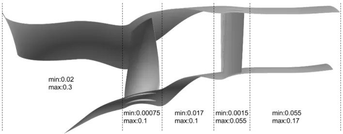
The process of mesh generation starts with the definition of connectors. The connectors are laid along the edges of the domain with an optimal point spacing based on experience to capture the geometry and some expected flow features. They can be laid within surfaces, as well, if control of point spacing in regions of such surfaces is difficult. Some of the point spacings (in inches) used on the stage are shown in Figure 4.1. This gives an idea of the level of surface mesh refinement when considering that the fan rotor diameter is 22 in.
Figure 4.1 Minimum and maximum point spacing used in different regions of the turbofan stage
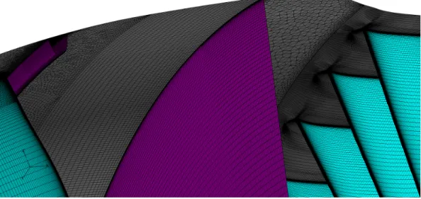
Following the definition of the edges is the creation of surface meshes. All domain bound-aries are represented by surface meshes, whether solid or permeable. Since unstructured meshes are used in this work, the surface meshes are composed by triangles and are defined by a set of connectors. The mesh generation software provides control of the arrangement of points on surface meshes, and it also allows for gradual increase of point spacing in a certain direction away from
the defining connectors. This is useful when creating viscous layers off solid surfaces. Figure 4.2 depicts the final surface mesh on the turbofan stage used for the majority of this work.
(a) Rotor blades (b) Stator blades
Figure 4.2 Surface mesh on parts of stage
Next is the creation of volume meshes. There are three parts to this phase. The first phase is the definition of volume blocks enclosed by surface meshes, a process carried out manually. Secondly, the creation of viscous layers is included in the volume mesh to capture the viscous boundary layer. The mesh generation software possesses tools for this task. It requires provision of the spacing for the first viscous layer off the solid walls, a linear rate of growth for the subsequent layers, and the setting of a minimum and maximum number of layers to be included. The calculation
of the first layer spacing off the solid walls is provided by viscous flow theory based on the concept of the non-dimensional wall distance y+. Web based tools provided by universities and software companies are available to carry out these calculations seamlessly. For proper capturing of the boundary layer the value ofy+is set to 1, and for a Reynolds number 107the computed wall spacing is approximately 4.5×10⁻⁵inwhich is set as the height of the first viscous layer in the mesh. A growth rate of 1.25 is chosen based on experience of previous work with turbo-machinery. A minimum number of 10 layers is enforced, and a maximum number of 16 layers is allowed based on testing reported later in Chapter 6. The last part in this process after the extrusion of viscous layers is filling out the rest of the block with tetrahedron shaped cells. The software automatically takes care of this task by inserting cells, the size of which gradually changes from the minimum to the maximum point spacings on the surfaces of the block. Figure 4.3 shows Pointwise visualizations of the viscous layer extrusion and a cut into the finalized volume mesh around the studs.
After completing the mesh, the boundary and volume conditions are declared. The boundary conditions are set by selecting all the surface meshes that belong to a boundary and assigning them the desired name for that boundary. Similarly, the volume conditions are set by selecting the volume meshes and assigning them a desired name. Two volumes were set for the meshes in this work. The Rotor volume, which was to be set in a rotating frame of reference in the solver, and a Stator volume, to be set in a fixed frame. The Rotor volume had the following boundaries assigned to it: rotor hub, blades, rotor casing, rotor periodic A and B, rotor inflow, and rotor outflow. The Stator volume had the following boundaries assigned to it: stator hub, stator blades, stator casing, stator periodic A and B, stator inflow, and stator outflow. The periodic boundary partners were set as axisymmetric boundary conditions, and the rotor outflow and stator inflow were set as interpolative boundary partners between the Rotor and Stator volumes, also called sliding interfaces. Figure 4.4 is a depiction of the type of boundaries used on the surfaces of the stage mesh, where all the surfaces in color grey are set as solid boundaries. When studs were used in the simulation, another boundary called Studs was assigned to the Stator volume.
4.2.3 Detail of Interpolative Interface and Studs Volume Mesh
An important feature of the meshes used in this work is the location of the sliding interface and the volume mesh around the studs. In previous work with this turbo-machine performed at the SimCenter, the sliding interface between the Rotor and Stator volumes was located approximately halfway between the fan blades and the stator vanes. Creating surface and volumes meshes near this interface was relatively simple since the components of the stage that possess many details were not in the vicinity. Adding the studs on the casing near the trailing edge of the fan blades for use as casing treatment added a level of complexity for two reasons: (i) the need for a new sliding interface around the location of the studs, and (ii) making use of a separate volume mesh for the regions where studs were to be included.
Adding a second interface for the studs was necessary because the flow solver requires that structures like this be in a stationary frame, and the location of the studs is very near the blades in the Rotor volume, a rotating frame. Creating a separate volume mesh for the near vicinity of the studs had a strategic purpose related to the results of the simulations: any changes in the solutions and the flow-field could be attributed only to the introduction of the casing treatment and not to changes on the rest of the mesh brought about by the introduction of the casing treatment. Having a block that isolated the mesh around the studs allowed introducing the studs, modifying their geometry, and recreating the volume only within that block, while leaving the rest of the stage volume mesh untouched. Figure 4.5 shows (in pink) the sliding interface between the rotor and stator sections, and the sliding interface for the studs alone.
Figure 4.5 The two sliding interfaces used in earlier simulations are shown in pink, rotor blades and stator vanes are shown in light blue, and casing is shown in grey.
Initial simulations with two sliding interfaces were successful but run time increased dra-matically. Relative to simulations with a single sliding interface, using two sliding interfaces took approximately 30% longer to run. This motivated a work around alternative to using two such interfaces. It was decided that the main sliding interface be brought near the trailing edges of the fan blades, such that the studs were now part of the Stator volume instead of being located within the Rotor volume. A separate volume block could still be created for the studs region where the surface meshes defining the block, other than the surface on the casing and the studs, were constant. This allowed merging the studs volume block with the Stator volume exactly the same way every time a modification of the casing treatment was done. Figure 4.6 serves to visualize the details described above.
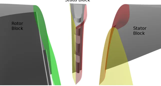
Figure 4.6 Surfaces separating the Rotor, Stator, and Studs volumes.
Figure 4.6 shows the surfaces separating the three blocks described in this section. All grey surfaces are actual solid surfaces. The green, yellow and red (mesh) surfaces remain unchanged with the modifications of the casing treatment geometry. The green surface is the sliding interface on the rotor side. The red surface meshes on each block are identical. When the Studs block and the Stator block are merged, the red surfaces are matched point to point and are unaccounted for once a single block is defined. Finally, once the Studs block and the Stator block are merged into a single one, the yellow surfaces become the single sliding interface on the stator side. When the baseline, smooth casing (no studs), case was tested, the ring shaped volume mesh (the “studs block” in Figure 4.6) contained no studs.
4.2.4 Finalizing the Mesh
Once the generation of the volume meshes is concluded, they can be exported with Pointwise into mesh files. Making the mesh files suitable for the flow solver is a process that requires the use of various software tools developed in-house. First, the meshes are checked for errors (i.e. negative volumes,“orphan” nodes) using the “gridcheck” tool. The next step is to merge the Studs and the Stator volume meshes into the complete Stator volume mesh using the “SUGG” (SimCenter unstructured grid generation) tool. Then, the Rotor and the Stator volume meshes are concatenated using the “gridcat” tool. Once the mesh files are finalized and suitable for simulation, the Rotor volume mesh contains about 7.5 million nodes and the Stator volume mesh contains about 8.6 million nodes, for a total of about 16.1 million nodes for the turbofan stage. Figure 4.7 shows a plane cut of all volume meshes across the sliding interface once they are merged and concatenated.
Figure 4.7 Aft-looking-forward view of volume mesh after generation and merging where the casing surface is shown in green, rotor blades and studs are depicted in pink, and a plane cut of the volume mesh is depicted in grey.
4.3 Setting Up and Running Cases
Once a mesh is ready, the next step is creating files that define for the solver the boundary conditions and the parameters the solver should use for performing computations. The SimCenter-developed software “TenasiGui” is used for this purpose. TenasiGui is a graphical user interface to the flow solver Tenasi designed to make the creation of the boundary and parameter files easy, and to provide tools to monitor the progress of the solution during run time.
The boundary condition file assigns boundary conditions to the surface boundaries defined in the mesh file. This is where the values of total pressure and total temperature are assigned to the rotor inflow boundary, where the back pressure is defined at the stator outflow, and where the solid walls are defined as adiabatic no-slip surfaces. The periodic surfaces are defined as axisymmetric boundaries, and the rotor outflow and stator inflow boundaries are matched as interpolative partners. This file also defines whether a volume mesh is set in a rotating or stationary frame of reference.
The parameters file defines the parameters the solver will use to perform the numerical simulations. This is where the solver is set to pick up initial conditions from another solution file or if the simulations are to be started from zero velocities in the flow-field, for example. The total number of steps and the time step size are defined here, as well as the number of steps to used first order spatial discretization before switching to second order. Reference values are specified, flow regime, turbulence model, and numerical schemes for solving the governing equations, just to name a few of the input parameters that are commonly needed.
Next is the decomposition of the mesh file, which is done using the SimCenter’s “decomp” tool. Required as inputs for mesh decomposition are the mesh file name, the length units used in
the mesh file, a case name, and the number of subdomains in which to decompose the mesh (which is the number of processors to be used for computation).
Finally, the cases are submitted to an in-house cluster for computation. Once submitted, some general computed values can be monitored from the file with the “.out” extension. Other files that record residuals, changes in solutions, and even timing are available for monitoring. Still other files are available to interact at run time with the solver to, for example, have the solver export solution files at any given time-step, or to terminate the run immediately, if so desired. If the simulation becomes unstable and computations are terminated, the flow solver will export files specifying the coordinate locations in the mesh where variable solutions became undefined or unrepresentable values (not-a-number, NaN). Furthermore, when using rotating frames of reference in the simulation, if the solver is unable to find points on a rotating frame, it will suspend the computations and export files providing locations of the “unfound” points.
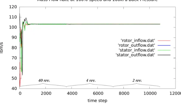
Once the solver finishes performing computations, information in the files provided by the solver can be extracted and analyzed to help decide whether running the case is concluded. In the present work, this is done by plotting the values of mass flow rate through the duct. When the plot shows the mass flow has remained essentially constant over several revolutions, it is deemed the solutions have arrived at convergence. Otherwise, the solver is re-started using the most recent solutions typically until the mass flow stabilizes. Figure 4.8 is an example of a mass flow plot indicating convergence of solutions. The figure shows that a first simulation of 40 revolutions was ran using 90 steps per revolution. The second simulation ran 4 revolutions using 900 steps per revolution. Finally, a third simulation ran 2 revolutions using 1800 steps per revolution.
Figure 4.8 Sample of mass flow computed across four boundaries in three consecutive simulations.
4.4 Post-Processing and Visualization
Once a case is completed, the solutions are post-processed and analyzed. First, the solution files, provided by each processor used in the computations, are recomposed into a single file using the SimCenter’s “recomp” tool. Then, the solutions in the flow-field can be visualized using the FieldView software [36] to observe the details of interest. FieldView can provide visualization of scalar and vector fields, depending on the type of information being analyzed. It also provides tools for extraction of data that may be of particular interest to the user. For example, in this work, such data has been velocity magnitudes, flow directions, pressure and temperature values, among others. GNUPlot [37] was used whenever such kind of data needed plotting for better analysis, and GNUPlot scripts were used to automate the process. Also, extraction of information from solution files was possible through development of Python scripts.
CHAPTER 5
RESULTS OF BASELINE SIMULATIONS
This chapter presents the results of the simulations of the fan stage with a smooth casing. Such results are compared against the experimental measures of performance of the SDT2-R4 to ensure an acceptable degree of agreement. This process is called validation, and achieving it is the first major part of this work and a very important step. The reason is that being able to computationally reproduce the experimental results provides a level of confidence in the results of the simulations for the modified geometry. It can then be said that the findings from this computational study resemble closely what would happen in a real case scenario. At this point, no casing treatment results are yet considered.
The performance values were calculated from simulations on the stage for corrected speeds of 100% and 87.5% of the design speed, which is 12,657 RPM. The quantities used to calculate the performance were mass flow, total pressure, and total temperature. Such quantities were integrated at the planes of the stage inlet, at the fan exit rake, and at the stator exit rake, as documented by Hughes [2] and shown in Figure 5.1. Also, the computed values presented here are for a range from the choke point (maximum mass flow) to a mass flow rate similar to that presented in the experimental results (92.1 lbm/s approximately).
Figure 5.1 Planes of integration of mass flow, total pressure and total temperature.
5.1 Performance Maps 5.1.1 Fan Performance
The pressure ratio, temperature ratio, and adiabatic efficiency curves for the fan rotor only are given in Figures 5.2, 5.3 and 5.4, respectively. The values used for their calculation were integrated at the stage inlet and at the fan exit only. The values of adiabatic efficiency were calculated using total pressure and total temperature values, and equation 5.1. The experimental values were obtained from Hughes [2].
ηad =
(p2/p1)(γ−1)/γ−1 (T2/T1)−1
(5.1)
The performance curves from the simulation are observed to closely resemble the experi-mental results with a slight over-prediction at both speeds. The trends of the pressure ratio curves are similar, only shifted up by an average of 0.95% for the 87.5% speed line and 0.50% for the
![Figure 2.2 Relation between systems and control volumes [1].](https://thumb-us.123doks.com/thumbv2/123dok_us/1877238.2774067/27.918.262.634.152.453/figure-relation-systems-control-volumes.webp)