Importance of the nozzle-exit boundary-layer state in subsonic turbulent jets

HAL Id: hal-02378471

https://hal.archives-ouvertes.fr/hal-02378471

Submitted on 25 Nov 2019

HAL

is a multi-disciplinary open access

archive for the deposit and dissemination of

sci-entific research documents, whether they are

pub-lished or not. The documents may come from

teaching and research institutions in France or

abroad, or from public or private research centers.

L’archive ouverte pluridisciplinaire

HAL

, est

destinée au dépôt et à la diffusion de documents

scientifiques de niveau recherche, publiés ou non,

émanant des établissements d’enseignement et de

recherche français ou étrangers, des laboratoires

publics ou privés.

Importance of the nozzle-exit boundary-layer state in

subsonic turbulent jets

Guillaume Brès, Peter Jordan, Vincent Jaunet, Maxime Le Rallic, André

Cavalieri, Aaron Towne, Sanjiva Lele, Tim Colonius, Oliver Schmidt

To cite this version:

Guillaume Brès, Peter Jordan, Vincent Jaunet, Maxime Le Rallic, André Cavalieri, et al..

Impor-tance of the nozzle-exit boundary-layer state in subsonic turbulent jets. Journal of Fluid Mechanics,

Cambridge University Press (CUP), 2018, 851, pp.83-124. �10.1017/jfm.2018.476�. �hal-02378471�

Importance of the nozzle-exit boundary-layer

state in subsonic turbulent jets

Guillaume A. Br`

es

†

, Peter Jordan

, Vincent Jaunet

, Maxime Le

Rallic

, Andr´

e V. G. Cavalieri

, Aaron Towne

, Sanjiva K.

Lele

, Tim Colonius

and Oliver T. Schmidt

1

Cascade Technologies Inc., Palo Alto, CA 94303, USA 2

Institut PPRIME, CNRS-Universit´e de Poitiers-ENSMA, Poitiers, France 3

Divis˜ao de Engenharia Aeron´autica, Instituto Tecnol´ogico de Aeron´autica, 12228-900 S˜ao Jos´e dos Campos, SP, Brazil

4

Center for Turbulence Research, Stanford University, Stanford, CA 94305, USA 5

Dept. of Mechanical Engineering and Dept. of Aeronautics & Astronautics, Stanford University, Stanford, CA 94305, USA

6

Division of Engineering and Applied Science, California Institute of Technology, Pasadena, CA 91125, USA

(Received ?; revised ?; accepted ?. - To be entered by editorial office)

To investigate the effects of the nozzle-exit conditions on jet flow and sound fields, large-eddy simulations of an isothermal Mach 0.9 jet issued from a convergent-straight nozzle are performed atdiameter-basedReynolds number 1×106_{. The} simu-lations feature near-wall adaptive mesh refinement, synthetic turbulence, and wall mod-elling inside the nozzle. This leads to fully turbulent nozzle-exit boundary layers and results in significant improvements for the flow-field and sound predictions, compared to those obtained from the typical approach based on laminar flow in the nozzle. The far-field pressure spectra for the turbulent jet match companion experimental measurements, which used a boundary layer trip to ensure a turbulent nozzle-exit boundary layer, to within 0.5 dB for all relevant angles and frequencies. By contrast, the initially laminar jet results in greater high-frequency noise. For both initially laminar and turbulent jets, de-composition of the radiated noise in azimuthal Fourier mode is performed and the results show similar azimuthal characteristics for the two jets. The axisymmetric mode is the dominant source of sound at the peak radiation angles and frequencies. The first three azimuthal modes recover more than 97% of the total acoustic energy at these angles and more than 65% (i.e., error less than 2 dB) for all angles. For the main azimuthal modes, linear stability analysis of the near-nozzle mean-velocity profiles is conducted in both jets. The analysis suggests that the differences in radiated noise between the initially laminar and turbulent jets are related to the differences in growth rate of the Kelvin-Helmholtz mode in the near-nozzle region.

Key words:

1. Introduction

For jets, the state of the boundary layer at the nozzle exit is well recognized as an important parameter of the flow development and noise radiation. It has been the focus

2 G. A. Br`es et al.

of many experimental studies, including works from Bradshawet al. (1964), Hill et al. (1976), Hussain & Zedan (1978b,a), Husain & Hussain (1979), Zaman (1985) and Bridges & Hussain (1987), as well as more recent studies by Zaman (2012), Karon & Ahuja (2013) and Fontaine et al. (2015). For full-scale nozzles at practical operating conditions, the nozzle-diameter based Reynolds number isRe =_O(107_{), implying turbulent boundary} layers and shear layers in the near-nozzle exit region. There is still debate about how thin the boundary layers are in a realistic engine context, as internal engine components will have non-trivial effects on the boundary layer development. On the other hand, in the context of idealized single-stream nozzles typically used for fundamental studies, these high-Reynolds-number features, important for the overall flow physics, remain challeng-ing to capture.

In terms of numerical studies, various forms of the direct numerical simula-tion (DNS) and large-eddy simulasimula-tion (LES) technique have been used over the years for jet flow and noise predictions. These research efforts have led to the availability of a substantial amount of data on compressible turbulent jets in general and, more specifically, on the influence of inflow conditions on the flow field and radiated noise. DNS studies can provide some valuable physics insights, but resolution requirements and computational costs restrict the simulations to Reynolds number of the order of103 _{to 10}4 _{(Freund 2001;}

Suponitsky et al. _{2010; Sandberg} et al. _{2012; B¨uhler} et al. ₂₀₁₄a_,b_{). The}

latter authors investigated Mach 0.9 laminar and turbulent nozzle-jet flows at Re = 18,100 and proposed empirical scalings to account for the reduced Reynolds number and lower turbulence levels, and correct the sound pre-dictions. As reviewed by Bodony & Lele (2008), a larger body of work is available on large-eddy simulation of jet flows. In the early LES studies (e.g., Morris et al. 2002; Uzun et al. 2004; Bodony & Lele 2005; Bogey & Bailly 2005), the nozzle geometry was typically not considered and simulations relied on the introduction of disturbances at the inlet of the computation domain to force transition. To avoid the specification of tunable parameters for the forcing and the potential spurious noise as-sociated with this, most recent simulations explicitly include a geometry at the inlet. However, inclusion of the physical geometry leads to challenges associated with the cor-rect simulation of the boundary layers inside the nozzle. Turbulent boundary layers are difficult to resolve in LES due to the substantial cost of simulating the full range of flow scales that are present(Choi & Moin 2012), to be added to the necessary cost of resolving the noise-source containing region at least 15 diameters downstream of the nozzle exit.

While early attempts were made to simulate initially turbulent jets (Uzun & Hussaini 2007; Bogeyet al. 2008), the computational expense of wall-resolved LES in the nozzle was prohibitive until recently. By now, Bogey & Marsden (2016) performed simulation of a Mach 0.9 jet issued from a straight pipe nozzle at Reynolds number 2_×105_{, which} featured transitional turbulent nozzle-exit boundary layers, but this required a grid of 3.1×109 _{points. An early attempt at wall-modelled LES was made by Anderssonet al.} (2005), where the Reynolds number for an isothermal Mach 0.75 was increased from 50,000 to 900,000, matching the value of a companion experiment. This was achieved on a structured grid of 30×106 _{points through the use of a wall function near the nozzle} walls, though the grid was too coarse to resolve even the outer portion of the turbulent boundary layer in the nozzle.

Most of the current LES are therefore performed at reduced simulated Reynolds num-ber, and the flow inside the nozzle is computed either through a coupling with Reynolds-averaged Navier-Stokes (RANS) calculations (Shuret al. 2005a,b, 2011), or, more com-monly, directly in the LES. In the latter case, the laminar flow issued from the nozzle

mixes with the ambient fluid at the nozzle exit and quickly transitions to turbulence. However, in this situation, the laminar shear layers allow enhanced coherent shear flow dynamics in the transition region, which can lead to an increase in sound associated with the vortex roll-up and pairing process. In these cases, special treatment of the noz-zle boundary layer is required, such as the introduction disturbances near the noznoz-zle exit. Bogey and coworkers considered, in a series of papers, the role of inflow conditions and initial turbulence on subsonic jets originating from a straight cylindrical pipe at

Re = 105_{, with LES on structured grids with up to 255}

×106 _{points (Bogey & Bailly} 2010; Bogey et al. 2011, 2012). The initially laminar jet boundary layers were tripped inside the pipe, upstream of the nozzle exit, by adding either low-amplitude random pressure disturbances or low-level random vortical disturbances decorrelated in the az-imuthal direction. The magnitude of the disturbances were empirically chosen to achieved targeted levels of peak turbulence intensity at the nozzle exit. Overall, they showed that these approaches weakened the coherent vortex pairing, increased the jet core length, and reduced the over-prediction of far-field noise spectra down towards those observed in experiments. As an alternative to this numerical forcing approach, Lorteauet al.(2015) used a geometrical tripping procedure (Pouangu´eet al.2012) in the simulation of a Mach 0.7 jet atRe= 4_×105_{on a structured grid with 275}

×106_{points.Vuillotet al.(2016)} extended the approach to unstructured grids and simulated the same case on a 183_×106 _{cell mesh. In both studies,the geometrical trip consisted of a small}

axisymmetric step added onto the surface inside the nozzle, reminiscent of boundary layer trip procedures used in experiments. It is argued that this method generates more natural turbulence, at the expense of additional constraints and tuning in the meshing process in order to robustly and efficiently integrate the added geometry with appropri-ate parameters.In terms of far-field noise, both LES studies showed that the geometrical trip was successful in reducing over-predicted spectra, within a few dB of experimental measurements.

The philosophy of the present study is to simulate the full scale system, including the turbulent flow inside the nozzle at the true Reynolds number and its effects on the nozzle-exit boundary layer, on the flow-field in the jet plume and ultimately on the acoustic field, using a predictive LES approach. This is achieved by leveraging recently developed wall model, synthetic turbulence method, and localized adaptive grid refinement approach.

The manuscript is organized as follows. The experimental configuration and numerical setup are reviewed in_§2, along with the modelling approaches used inside the nozzle (i.e., near-wall adaptive mesh refinement, synthetic turbulence seeding and wall modelling). Then, in_§3, results from a series of preliminary large-eddy simulations are discussed to highlight the separate and combined effects of the different approaches used to simulate the internal nozzle flow. Further validation and analysis of the down-selected cases with initially laminar and fully turbulent nozzle-exit boundary layers are presented in _§4, including azimuthal Fourier decomposition of the radiated sound. For the main azimuthal modes, linear stability analysis of the near-nozzle mean velocity profiles is conducted to investigate the differences in far-field noise between the two jets. Concluding remarks and future directions are discussed in§5.

2. Flow configuration and numerical methods

The study focuses on isothermal subsonic jets issued from a round nozzle of exit diameter

4 G. A. Br`es et al.

the Institut PPRIME, Poitiers, France. Boundary layer transition inside the nozzle is forced using an azimuthally homogeneous carborundum strip of width 0.28D, whose downstream edge is located approximately 2.5D from the nozzle exit. The operating conditions are defined in terms of the nozzle pressure ratioN P R =Pt/P∞ = 1.7 and

nozzle temperature ratio N T R = Tt/T∞ = 1.15. Here, the subscripts t and ∞ refer

to the stagnation (total) and free-stream (ambient) conditions, respectively. The jet is isothermal (Tj/T∞ = 1.0), and the jet Mach number is Mj = Uj/cj = 0.9, where U is the mean (time-averaged) jet exit streamwise velocity, c is the speed of sound and the subscriptj refers to jet properties. With these conditions, the Reynolds number is

Re=ρjUjD/µj≈1×106.

Details about the nozzle geometry, experimental configuration and noise post-processing procedure are reported in Appendices A and B. Some of these details are also available in the supplemental materials, along with measurements and LES data.

2.2. Numerical setup

The present simulations use the LES framework developed at Cascade Technologies and leverage recent research efforts focused on modelling of the nozzle-interior turbu-lence (Br`eset al. 2013, 2014). The framework is composed of the pre-processing mesh-adaptation tool “Adapt”, the compressible flow solver “Charles,” and post-processing tools for far-field noise predictions based on an efficient massively-parallel implementation of the frequency-domain permeable formulation (Lockard 2000) of the Ffowcs Williams & Hawkings (1969) (FW-H) equation.Charles solves the spatially-filtered compress-ible Navier–Stokes equations on general unstructured grids using a density-based finite-volume method. Time integration is explicit and uses the third-order TVD RK scheme of Gottlieb & Shu (1998). The compressible fluxes are computed using a blend of central and upwind flux, resulting in a nominally 2nd-order scheme in space. The computational setup is briefly summarized below, with additional details about the solvers, the numerical schemes and the basic methodology available in Br`es et al. _{(2017). Note that this reference}

does not cover the issues related to nozzle-interior turbulence modellings, which are the focus of the present work and are discussed in detail in what follows.

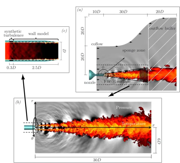
Schematics of the numerical setup are presented in figure 1, along with visualization of the instantaneous temperature and pressure field. The round nozzle geometry (with exit centered at (x, r) = (0,0)) is explicitly included in the axisymmetric computational domain, which extends from approximately₋10Dto 50Din the streamwise (x) direction and flares in the radial direction from 20Dto 40D. A very slow coflow at Mach number

M∞= 0.009 is imposed outside the nozzle in the simulation (M∞= 0 in the experiment),

to prevent spurious recirculation and facilitate flow entrainment. All other simulation settings match the experimental operating conditions, including the Reynolds number. The Vreman (2004) sub-grid model is used to account for the physical effects of unresolved turbulence on the resolved flow,with constant coefficient set to the recommended value of c = 0.07. A constant turbulent Prandtl number P rt = 0.9 is used to close the energy equation.To avoid spurious reflections at the downstream boundary of the computational domain, a damping function (Freund 1997; Mani 2012) is applied in the outflow buffer zone as a source term in the governing equations. In addition, the numerical operators are switched to lower-order dissipative discretization in the sponge zone forx/D >31 andr/D >7, to further damp turbulent structures and sound waves. Unless specified otherwise, all solid surfaces are treated as no-slip adiabatic walls.

(c)

D

2.5D

0.3D

synthetic

turbulence wall model

(a) coflow sponge zone outflow buffer FW-H surface nozzle 2 0 D 2 0 D 10D 30D 20D φ (b) 6 D 30D x r θ Pressure Temperature

Figure 1. (Colour online) Schematics of the flow configuration and simulation setup: (a) overview of the computational domain; (b) spatial extent of the LES database; (c) modelling inside the nozzle.

nozzle exit was calculated for three different FW-H surfaces consisting of a cylindrical surface of radius 0.65D up x/D = 0, followed by a conical surface extending to x/D = 30 with different spreading rates of 0.11, 0.14 and 0.17. Here, the slopes are chosen based on estimates of the jet spreading rate (Za-man 1998, 1999).Similarly to previous studies (Br`eset al. 2017), the results showed nearly identical spectra over the main frequency range for the three surfaces. The ro-bustness of the prediction being thus confirmed, only the results from the intermediate surface outlined in black in figure 1(a)are reported. For treatment of the FW-H outflow disk, the method of “end-caps” of Shur et al. (2005a) is applied for x > 25D, where the complex far-field pressure predicted from eleven FW-H surfaces with the same shape but outflow disks at different streamwise locations are phase-averaged. For all cases, the sampling period of the data recording on the FW-H surface is ∆tF W Hc∞/D= 0.05.

Table 1 lists the settings and parameters for each LES run considered, including the time stepdt, the total simulation timetsim (after the initial transient is removed), and the data sampling period ∆t for the cases where the LES database of the full 3D flow field in primitive variable (ρ, P, u, v, w)was collected, all expressed in acoustic time units (i.e., non-dimensionalized by c∞/D). The total computational cost is

6 G. A. Br`es et al.

Mesh Grid Synthetic Wall dtc∞ D t_simc∞ D ∆tc∞ D CPU

Case name size refinement turbulence model cost

(106 cv) BL Jet u′ trip/uτ (kcore-h) Baseline LES 10M 10.8 0.001 2000 40 64M 64.2 × 0.0005 600 464

LES with nozzle-interior turbulence modelling

BL16M 15.9 × 0.001 600 59 BL16M Turb2 15.9 × 2 0.001 600 69 BL16M Turb 15.9 × 0.8 0.001 600 69 BL16M WM 15.9 × × 0.001 600 75 BL16M WM Turb2 15.9 × 2 × 0.001 600 81 BL16M WM Turb 15.9 × 0.8 × 0.001 2000 0.2 270 BL69M WM Turb _69.0 × × 0.8 × 0.0005 1150 0.2 1514 Table 1.Simulation parameters: synthetic turbulence amplitudeA=u′

trip/uτ, time stepdt, total simulation timetsim, and database sampling period ∆t

also reported in thousand core-hours. All the calculations were carried out on the Cray XE6 system “Garnet” (Opteron 16C 2.5GHz processors, Cray Gemini interconnect, theoretical peak of 1.5 TFlop/s) on 1024 cores and 5152 cores for the standard and refined grids, respectively. The simulations with nozzle-interior turbulence modelling focused on adaptive isotropic mesh refinement of the internal boundary layer (prefix BL_{), synthetic turbulence (suffix} Turb_{), and wall}

modelling inside the nozzle (suffixWM_).

2.3. Mesh adaptation and near-wall refinement

The current meshing strategy has been used in previous jet studies (Br`eset al.2013, 2014, 2015, 2016) and promotes grid isotropy in the acoustic source-containing region through the use of adaptive refinement. The starting point is a coarse structured cylindrical grid with a paved core andclustering of points in the radial direction at the nozzle walls and lip. The grid contains about 0.4 million purely-hexahedral control volumes. Several embedded zones of refinement with specific target length scale∆are then defined by the user, and enforced iteratively by the adaptation tool, such that any cell with edge length (in any direction) greater than∆ will be refined in that direction, until the target length scale criterion is satisfied. The main refinement zone corresponds to the bulk of the mesh containing the jet plume, from (x/D, r/D) = (0,1.5) to (30,5), with ∆/D = 0.14. Then, within that zone, three additional conical refinement regions focusing on the jet potential core and surrounding the FW-H surface are defined, from the nozzle lip to (x/D, r/D) = (10,2.5), (7.5,2) and (5.5,1.5), with ∆/D = 0.1, 0.07 and 0.04, respectively. Finally, near the nozzle exit, three more refinement windows are centered on the lipline, extending to x/D = 2, 0.7 and 0.5, with ∆/D= 0.02, 0.01 and 0.0058, respectively.

For the baseline cases, two grids were generated: a standard mesh containing approxi-mately 10 million unstructured control volumes (cvs), and a refined mesh with 64 million cvs, by reducing the target length scale in half in each refinement zone in the jet plume. Note that for these cases, there is no specific near-wall or nozzle-interior refinement, and both grids have exactly the same coarse resolution inside the nozzle.

10−1 10−2 10−3 0 0.5 (a) x/D=−1 10M 64M D im en si o n le ss m es h sp a ci n g 10 −1 10−2 10−3 0 0.5 1 (b) x/D= 0 10M BL16M 10−1 10−2 10−3 0 0.5 1 1.5 (c) x/D= 2 10M BL16M 10−1 10−2 10−3 0 0.5 D im en si o n le ss m es h sp a ci n g x/D=−1 BL16M BL69M r/D 10−1 10−2 10−3 0 0.5 1 x/D= 0 64M BL69M r/D 10−1 10−2 10−3 0 0.5 1 1.5 r/D x/D= 2 64M BL69M

Figure 2.(Colour online) Dimensionless mesh spacing (a) inside the nozzle atx/D=−1, (b) at the nozzle exitx/D= 0 and (c) atx/D= 2, in the axial (∆x/D ), radial (∆r/D ), and azimuthal (r∆θ/D ) directions, and equivalent cell length (vol1_/3

/D ◦ ) for the grid10M(top) andBL69M(bottom). The grids with the same mesh spacing are also reported in the figures (see table 1).

10−1 10−2 10−3 0 5 10 15 (a) D im en si o n le ss m es h sp a ci n g x/D lipline 10M 64M 10M BL16M 10−1 10−2 10−3 0 5 10 15 (b) x/D lipline BL16M BL69M 64M BL69M

Figure 3.(Colour online) Dimensionless mesh spacing along the lipline atr/D= 0.5, in the axial (∆x/D ), radial (∆r/D ), and azimuthal (r∆θ/D ) directions, and equivalent cell length (vol1/3

/D ◦ ) for the grid (a)10M_{and (b)}BL69M_{. The grids with the}

same mesh spacing are also reported in the figures (see table 1).

be anticipated that further mesh refinement is needed inside the nozzle to resolve the large-scale three-dimensional turbulent structures associated with the internal boundary layers. Therefore, isotropic refinement is added to the previous adaptation strategy and applied from the start of the boundary layer trip at x/D =₋2.8 to the nozzle exit at

8 G. A. Br`es et al. 10−1 10−2 0 5 10 15 (a) D im en si o n le ss m es h sp a ci n g x/D FW-H outline 10M BL16M 10−1 10−2 0 5 10 15 (b) x/D FW-H outline 64M BL69M

Figure 4.(Colour online) Dimensionless mesh spacing along the conical FW-H outline, in the axial (∆x/D ), radial (∆r/D ), and azimuthal (r∆θ/D ) directions, and equivalent cell length (vol1/3

/D ◦ ) for the grid (a)10M_{and (b)}BL69M_{. The grids with the}

same mesh spacing are also reported in the figures (see table 1).

∆/D= 0.0075. The distance was chosen based on an initial estimate of the experimental nozzle-exit boundary layer thickness,δ99_{/D≈0.08, and the length scale was chosen to} yield about 10-20 LES cells in the boundary layer. These choices lead to a finest wall-normal resolution of approximately 0.004D, after adaption.As part of a preliminary study focusing solely on the flow inside the nozzle, additional simulations were performed on two grids where the target length scale for the near-wall refinement was reduced to0.0058and 0.0029, respectively. Theses simulations yielded only limited improvements in the internal boundary layer predictions for a significant increase in computational cost. Therefore, we chose the more practical approach of keeping the resolution inside the nozzle on the modest side for wall-bounded flows.Mesh details at the nozzle wall and lip are reported in table 2. The adapted grids with boundary layer refinement now contain approximately 16 million and 69 million cvs, for the standard and jet-plume refined cases, respectively. Figures 2, 3 and 4 show, in logarithmic scales, the dimensionless mesh spac-ings for the four grids at different streamwise locations, along the lipline and along the outline of the conical section of the FW-H surface, respectively.In contrast to fully structured grids, the mesh length scales for the present unstructured grids with adaptation and hanging nodes are not globally predefined with smooth an-alytical form and vary in space depending on the refinement target length scales. The location of the user-defined grid transitions are clearly visible in the figures, in particular for the azimuthal length scale (red solid curve) in figure 3 at x/D = 0.5, 2, 5.5, etc. . Nevertheless, the present isotropic refinement strategy leads to similar mesh spacing in all three axial, radial and azimuthal directions for most of the relevant regions of the computational domain. In terms of mesh isotropy, the only noticeable exception is near the lipline where the small radial resolution, present in the initial structured cylindrical grid to resolve the nozzle lip, remains in the adapted grids and leads to more anisotropy in the downstream region of the jet plume (see figure 3). The effect is however local-ized and overall, the cell aspect ratio (i.e., largest over smaller mesh length scale) is less than 2 for 85% (97%) of the control volumes within the FW-H surface, for the grid without (with) jet plume refinement. The equivalent cell lengthvol1/3_{/D, which is the} cubic-root of the cell volume, is therefore a representative metric of the resolution for the present isotropic hexahedral-dominant grids and is also presented in the figures. Follow-ing the analysis of Mendezet al. _{(2012) and Br`es} et al. _{(2017), this quantity}

Location Case prefix ∆x/D ∆r/D r∆θ/D vol1/3

/D nθ trip (x/D=−2.5) 10M_BL16M,64M_,BL69M 0.1000_{0.0062 0.0045}0.0090 0.0478_0.0059 0.0350_{0.0055 530}76 nozzle lip (x/D= 0) 10M_64M,_,BL16M_BL69M 0.0030_0.0015 0.0034_{0.0017 0.0015}0.0030 _0.00160.0031 1050₂₀₉₅ Table 2.Representative mesh spacing atr/D= 0.5 and corresponding number of grid points

in the azimuthal directionnθ

is also used to estimate the limit Strouhal numberStlim of acceptable resolu-tion, corresponding to a wave resolved with eight grid point per wavelength: Stlim = D/(8vol1/3Ma), where Ma =Uj/c∞ is the acoustic Mach number.

Be-cause the high-frequency noise sources are typically expected in the jet plume between the nozzle exit and the end of the potential (i.e., 0 < x .10), the present grids are designed to approximately resolve the radiated noise spec-tra up to Stlim ≈ 2 for the standard mesh and to Stlim ≈ 4 for the refined mesh, based on the resolution on the FW-H surface in that region.

2.4. Synthetic turbulence

An extension to the digital filtering technique of Kleinet al.(2003) was implemented for the generation of synthetic turbulence on unstructured grids,for both inflow bound-ary and wall boundbound-ary conditions.Because the turbulence levels inside the exhaust system upstream of the nozzle are typically unknown, the main objective of the synthetic turbulence is to seed the flow with fluctuations of reasonable amplitude, length and time scales, such that realistic turbulence is fully developed by the nozzle exit.

In the present work, synthetic-turbulence boundary conditions are used to model the boundary layer trip present in the experiment at ₋2.8 < x/D < ₋2.5 on the internal nozzle surface (see figure 1(c)). Based on the initial estimate of the experimental nozzle-exit boundary layer thickness, the trip is therefore located more than 30δ99_{/D from the} nozzle exit, which is sufficient for the spatial development of a turbulent boundary layer. The wall friction velocity uτ is often used as a scaling parameter for the fluctuat-ing component of velocity in wall-bounded turbulent flows. An initial value foruτ was estimated based on the average wall shear stress downstream of the trip location for preliminary simulation on the 16M mesh.Fluctuations are then introduced in each component of the zero-mean velocity field at the wall boundary faces of the trip, with a prescribed amplitude u′

trip = Auτ/√3. As part of the initial para-metric studies, two different amplitudes, A = 0.8 and 2, were used, with the former value applied for most of the computations. For all cases, ∆max and 2∆max/u′trip are used as initial estimates of the length and time scales of the input fluctuations, where ∆max = max(∆x,∆r, r∆θ) is the largest mesh spacing at the location of the trip (see table 2). Physically, this can be interpreted as the introduction of isotropic eddies of turbulent kinetic energy 1/2(Auτ)2 and dimensions comparable to the local mesh size. Here, the chosen length scale is also similar to the thickness of the experimental trip.

While the present work focuses on theMj = 0.9 case, different Mach number condi-tions ranging from 0.4 to 0.9 were considered as part of a broader LES study and nearly identical initial estimatesuτ/Uj≈0.042 were obtained in all cases. Similar values can be obtained using simple flat-plate zero-pressure-gradient turbulent boundary layer approx-imations. Assuming the classical form of the skin-friction coefficient in turbulent flows,

10 G. A. Br`es et al.

cf = 0.0576Re

−1/5

x , with xas the distance between the start of the straight section of the nozzle and the boundary layer trip, the empirical value of the wall friction velocity at the trip would be betweenuτ/Uj≈0.041 and 0.044 forMj = 0.9 to 0.4. These estimates further confirmed the choice of order-of-magnitude for the coefficientA=_O(1).

2.5. Wall modelling

When active, the equilibrium wall model, based on the work of Kawai & Larsson (2012) and Bodart & Larsson (2011), is applied inside the nozzle in the straight-pipe section be-tween the boundary layer trip and the nozzle exit (see figure 1(c)). The present method falls in the category of the wall-stress modelling approach (see reviews by Piomelli & Balaras 2002; Larssonet al.2016): unlike hybrid RANS/LES and detached-eddy simu-lations (Spalart 2009) that solve the unsteady Navier-Stokes equations on a single grid, with a RANS model near the wall and a LES model in the rest of the domain, the un-structured LES grid is formally defined as extending all the way to the wall (i.e., identical to a simulation without wall model), and a separate (structured) grid is embedded near the wall to solve the 1D RANS equations. The RANS solver takes information from the computed LES flow-field a few cells away from the wall, and returns back the shear stress

τw and the heat transferqw at the wall, to be used as boundary conditions for the LES wall-flux computation.

For most convex surfaces, the RANS grid is a simple extrusion of the wall surface mesh along the normal vector of each wall face. Following the recommendations of Kawai & Larsson (2012), the wall-model-layer thickness (i.e., the distance from the wall where the RANS solver takes the LES information) is set to at least three LES cells away from the wall.In previous work (Br`es et al._{2013), various sizes and stretching}

coefficients were considered for the inner-layer RANS grid and the default values of 40 cells and 10% stretching are used in the present study, for a wall-normal grid spacing in wall units y+_{RAN S} = _O(1). As shown in table 1, for the present cases with no specific attempt to optimize the performances, the extra computational cost of the wall model is about 27% of the stand-alone LES cost, similar to the value of 30% reported by Bodart & Larsson (2011). Load-balancing of the wall-model procedure has been suggested as an approach to potentially reduce this additional cost.

3. Parametric study of nozzle-interior turbulence modelling

First, a study of the separate and combined effects of near-wall adaptive mesh re-finement, the introduction of synthetic turbulence, and wall modelling is conducted on the standard mesh. To provide consistent comparisons, the same total simulation time

tsimD/c∞ = 600 is used for the computation of the flow statistics and far-field noise

spectra presented in this section. Down-selected cases are then simulated for an extended period and discussed in_§4.

3.1. Effects of nozzle-interior turbulence modelling on flow field results 3.1.1. Instantaneous flow field

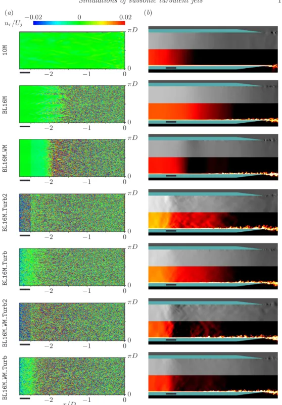
Figure 5 shows the instantaneous flow inside the nozzle for the various cases with and without nozzle-interior turbulence modelling. Recall that both baseline cases 10M _and 64M_{have the same operating conditions and same coarse mesh inside the nozzle. This}

leads to the same internal flow field and thin laminar boundary layer, with no visible velocity fluctuations inside the nozzle (see top row in figure 5).

1 0 M (a) (b) 0 0 −1 −2 πD ur/Uj −0.02 0 0.02 B L 1 6 M 0 0 −1 −2 πD B L 1 6 M W M 0 0 −1 −2 πD B L 1 6 M T u r b 2 0 0 −1 −2 πD B L 1 6 M T u r b 0 0 −1 −2 πD B L 1 6 M W M T u r b 2 0 0 −1 −2 πD B L 1 6 M W M T u r b 0 0 −1 −2 πD x/D

Figure 5.(Colour online) Instantaneous flow field inside the nozzle, for the baseline LES 10M

(top row) and LES with nozzle-interior turbulence modelling: (a) Wall-normal velocityur/Ujin the first cell near the (unrolled) nozzle interior surface. When active, the synthetic turbulence is applied for−2.8< x/D <−2.5 ( ); (b) pressure (top half - grey scale) and temperature field (bottom half - red scale) in the mid-section plane inside the nozzle. The colour ranges are

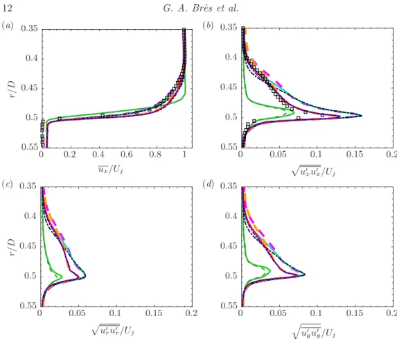
12 G. A. Br`es et al. ux/Uj r/ D 0.55 0.5 0.45 0.4 0.35 0 0.2 0.4 0.6 0.8 1 (a) p u′ xu′x/Uj 0.55 0.5 0.45 0.4 0.35 0 0.05 0.1 0.15 0.2 (b) p u′ ru′r/Uj r/ D 0.55 0.5 0.45 0.4 0.35 0 0.05 0.1 0.15 0.2 (c) q u′ θu ′ θ/Uj 0.55 0.5 0.45 0.4 0.35 0 0.05 0.1 0.15 0.2 (d)

Figure 6.(Colour online)Nozzle-exit boundary layer profiles atx/D = 0.04of (a) the mean streamwise velocity and (b-d) the RMS values of the fluctuating velocity components: experiment ( hot-wire), baseline LES10M ( ) and 64M ( ), and LES with noz-zle-interior turbulence modellingBL16M( ),BL16M Turb2( ),BL16M Turb ( ),

BL16M WM( ),BL16M WM Turb2( ) andBL16M WM Turb( ).

a significant impact for the present configuration. All the simulations with isotropic near-wall grid refinement display small-scale three-dimensional turbulent structures in the boundary layer.Depending on the addition of synthetic turbulence and/or wall modelling, the development of turbulence near the walls and in the nozzle core flow differs. Without synthetic turbulence, the internal boundary layer undergoes transition over a long stretch of the nozzle for the case BL16M_{, and more uniformly around x/D = −2 for the case} BL16M WM_{with wall modelling. With synthetic turbulence, more fluctuations are visible} in the pressure and temperature field in the vicinity of the trip, in particular for the cases with the high amplitude coefficient (i.e., suffix Turb2_{). However, the flow field} within the last one diameter before the nozzle exit looks qualitatively similar in all cases with nozzle-interior turbulence modelling.

3.1.2. Nozzle-exit velocity statistics

Nozzle-exit profiles of velocity statistics are plotted in figure 6. Both experimental hot-wire measurements and LES results are reported at the same location just downstream of the nozzle exit, atx/D= 0.04. The slight mismatch in mean velocity forr/D >0.5 is caused by the small coflowM∞= 0.009 imposed in the simulation.

For both baseline cases, the mean (time-averaged) streamwise velocity profiles are identical and correspond to the typical laminar profile. The turbulence intensities in

figure 6(b-d) all show similar characteristics, with a single wider peak and lower RMS values. In contrast, the nozzle-exit boundary layer in the experiment is turbulent, thanks to the azimuthally homogeneous carborundum strip upstream in the pipe. The RMS peaks are therefore largely under-predicted and the boundary layer is too thin for both LES10M_and64M_.

With isotropic near-wall grid refinement, all the nozzle-exit boundary layers now ex-hibit turbulent mean and RMS velocity profiles, with larger fluctuation levels near the wall. Much like the nozzle-exit boundary layer measurements of Fontaine et al.(2015), the present turbulence intensity profiles feature two distinct regions. The first region, which Fontaineet al. (2015) refer to as the “boundary layer remnant”, is characterized by a relatively shallow rise, up tor/D≈0.47 in our study. This region is here present in both experiment and simulations, and, for the simulation, is sensitive to the amplitudes of synthetic turbulence and/or presence of wall modelling. The second region, which they associate with the inflectional instability of the free shear profile, is characterized by a sharp peak in RMS levels nearr/D≈0.5. In that region, the LES results collapse onto two distinct curves, depending on whether or not wall modelling is used. While the nozzle-exit RMS levels are over-predicted compared to experiment for casesBL16M_,

BL16M Turb_andBL16M Turb2_{(see Figure 6(b)), the cases with wall modelling show less}

overshoot and better agreement. Here, the effect of the wall model is significant and beneficial: the most important region in terms of the initial growth rate of wavepackets is this “shear-layer” region, where the correct RMS underpins the correct velocity gradi-ent. Over-prediction of near-wall fluctuations is a characteristic feature of under-resolved LES. Even the present choice of 20 points across the nozzle-exit boundary layer thickness is coarse in terms of viscous units at the wall.Based on the resolution in the first LES cell from the nozzle internal surface, the wall-normal grid spacing in wall unitsyLES+ is in the 130 to 175 range, and about 200 to 240 for the streamwise and azimuthal grid spacing, depending on the case and streamwise location. In a corresponding DNS, the typical values would be about 1 in the normal direction, 10 to 20 in the streamwise direction and 5 to 10 in the azimuthal direction. Therefore, the turbulent boundary layer needs to be in the wall-modelled LES regime. The physics in the viscous sublayer are now wall-modelled with the 1D RANS, leading to an average y+_{RAN S ≈} 0.7 for the first RANS cell.

Finally, the addition of synthetic turbulence has less impact than mesh refinement and wall modelling. Two different levels of amplitudes for the synthetic turbulence were tested (see table 1), and the change in fluctuation amplitude can clearly be seen in figure 5 at the location of the trip, for instance in casesBL16M Turb_andBL16M Turb2_{. However, as more}

realistic turbulence develops, the differences in flow structures at the wall only persist for about 0.5D downstream of the trip, and visually similar turbulent boundary layers are then observed beyond that point. As shown in figure 6, the nozzle-exit boundary layer profiles in the “shear-layer” region are essentially independent of the initial choice (or absence) of synthetic fluctuations. The main discernable differences are observed in the “boundary layer remnant”, where the turbulence levels in the nozzle core flow away from the walls are slightly larger with the high amplitude synthetic turbulence.

3.1.3. Centerline and lipline profiles

The streamwise velocity statistics along the centerline and lipline (i.e., r/D = 0.5) in figure 7 also show improved results for the LES cases with nozzle-interior turbulence modelling. The most drastic change can be observed in the fluctuation amplitude along the lipline in figure 7(d) where the fluctuation overshoot aroundx= 0.5D(related to the

14 G. A. Br`es et al. ux / Uj p 0.2 0.4 0.6 0.8 1 0 5 10 15 20 (a) centerline 0.95 1 1.05 −1 −0.5 0 0 0.2 0.4 0.6 0.8 0 5 10 15 20 (b) lipline 0 0.5 1 1.5 2 0 0.2 0.4 0.6 p u ′ux ′/_x Uj x/D 0 0.05 0.1 0.15 0 5 10 15 20 (c) centerline 0 5 −1 −0.5 0 ×10−3 x/D 0 0.05 0.1 0.15 0.2 0 5 10 15 20 (d) lipline 0.1 0.15 0.2 0 0.5 1 1.5 2

Figure 7.(Colour online) Profiles along the centerline and lipline of (a,b) mean and (c,d) RMS streamwise velocity: experiment ( hot-wire, ◦ PIV), baseline LES 10M ( ) and 64M

( ), and LES with nozzle-interior turbulence modelling BL16M ( ), BL16M Turb2

( ),BL16M Turb( ),BL16M WM( ),BL16M WM Turb2( ) andBL16M WM Turb

( ).

shear-layer laminar-to-turbulent transition) is present in both baseline LES, independent of the resolution in the jet plume, but is nearly removed with improved treatment of the internal nozzle dynamics.

For the centerline profiles, the main feature is the under-prediction of the length of the potential corexc (defined as the distance up to which the streamwise velocity is greater than 95% of the jet exit velocity) for the baseline case10M_{. The early termination of the}

potential core results in the shift of the peak RMS levels further upstream. As expected, the grid refinement in the jet plume for case 64M _{slightly improves the prediction of}

turbulent mixing, and of xc, but the RMS levels remains well under-predicted. Better improvements are actually obtained on the standard mesh for all the cases with nozzle-interior turbulence modelling. Inside the nozzle, all the simulations show very low nozzle core-turbulence levels (see insert in figure 7(c)). As discussed in the previous section, slightly larger values are observed for the two cases with high initial amplitude of the synthetic turbulence (i.e., suffixTurb2₎

Overall, the wall-modelled LES cases provide arguably the best match with the PIV measurements, in particular in the very-near nozzle region x/D <0.5. Due to the rela-tively short simulation time used for these preliminary comparisons, the statistics shows some variations between the different cases, in particular for x/D > 8, in the fully-developed mixing jet region downstream of the potential core, where the statistics are more significantly underpinned by low-frequencies, difficult to converge with the short

0.1 1 10 130 140 150 (a) (x/D, r/D) = (−0.05,0.48) P S D ( P ′) (d B / S t) 0.1 1 10 140 150 160 170 (b) (x/D, r/D) = (0.5,0.5) 0.1 1 10 140 150 160 170 (c) (x/D, r/D) = (5,0.5) −7/3 0.1 1 10 10−5 10−3 P S D ( u ′)x 0.1 1 10 10−5 10−3 10−1 0.1 1 10 10−5 10−3 10−1 −5/3 0.1 1 10 10−5 10−3 P S D ( u ′)r 0.1 1 10 10−5 10−3 10−1 0.1 1 10 10−5 10−3 10−1 −5/3 St 0.1 1 10 10−5 10−3 P S D ( u ′)θ St 0.1 1 10 10−5 10−3 10−1 St 0.1 1 10 10−5 10−3 10−1 −5/3

Figure 8.(Colour online) Spectra of pressure and velocity fluctuations along the lipline (a) at (x/D, r/D) = (−0.05,0.48), (b) (0.5,0.5) and (c) (5,0.5): baseline LES10M ( ) and 64M

( ), and LES with nozzle-interior turbulence modelling BL16M ( ), BL16M Turb2

( ),BL16M Turb( ),BL16M WM( ),BL16M WM Turb2( ) andBL16M WM Turb

( ). The arrows indicate the frequencies of the trapped acoustic waves (see Appendix C). simulation time. Higher-order moments such as RMS and skewness are, of course, more sensitive to statistical convergence and spatial resolution. Specifically, some of the sharp changes in slope in the RMS profiles are related to transitions in mesh resolution, as cor-roborated by the mesh spacing curves in figure 3. These features are discussed in greater details in _§4.1 for the LES with extended simulation time and additional refinement in the jet plume.

3.1.4. Pressure and velocity fluctuation spectra

Figure 8 shows the power spectral density (PSD) of the pressure fluctuations (in dB/St) and of the three components of the velocity fluctuations in cylindrical coordinates (non-dimensionalized by U2

j/St) as a function of frequency in Strouhal St = f D/Uj. The spectra are directly computed from the flow-field time histories recorded along the lipline

16 G. A. Br`es et al.

at (x/D, r/D) = (₋0.05,0.48), (0.5,0.5) and (5,0.5) for 36 equally-spaced locations in the

azimuthal direction. Because of the azimuthal symmetry of the geometry, these locations are statistically equivalent and the resulting spectra are azimuthally averaged.

The first position (x/D, r/D) = (₋0.05,0.48) is representative of the near-wall flow inside the nozzle. As expected, for the baseline cases10M_and64M_{with initially laminar} boundary layers, the velocity fluctuations have much lower levels and no discernible high-frequency content. In contrast, all the simulations with nozzle-interior flow modelling display turbulent spectra with broadband frequency content. For these cases, the velocity spectra collapse onto two curves of similar shape but different amplitude, depending on whether wall modelling is applied or not. As mentioned in the previous section, over-prediction of near-wall fluctuations is a characteristic feature of under-resolved LES and all the simulations without wall modelling exhibit higher levels of velocity fluctuations. At this location, the velocity spectra are independent of the initial choice (or absence) of synthetic fluctuations, much like the nozzle-exit velocity profiles in the “shear-layer” region discussed in §3.1.2. In contrast, the pressure spectra show some sensitivity to the synthetic turbulence parameters. Namely, higher initial amplitude of the synthetic turbulence inside the nozzle leads to higher levels of pressure fluctuations in the mid-to high-frequency range. Here, another interesting feature is the presence of mid-tones in the pressure spectra at specific frequencies for all the simulations. Some of the tones are also visible in the velocity spectra of the baseline cases10M_and64M_{because of the low} fluctuation levels. These discrete tones are characteristics of a novel class of resonant acoustic waves which are trapped within the potential core of the jets and transmit some of the energy into the nozzle (see Appendix C).

The second position (x/D, r/D) = (0.5,0.5) corresponds to the location of peak RMS overshoot along the lipline related to the shear-layer laminar-to-turbulent transition in the baseline LES. Therefore, higher fluctuation levels are observed for both cases10M_and 64M _{with initially laminar jet, compared to all the other cases with initially turbulent} jet, in particular in the pressure spectra. For the simulations with nozzle-interior flow modelling, all the spectra now collapse on a single broadband curve, independently of the use of wall model or presence/initial amplitude of the synthetic turbulence inside the nozzle. Here, some of the tones associated with the trapped acoustic waves are still visible, while others have been overwhelmed by the increased turbulence levels.

The third position (x/D, r/D) = (5,0.5) is located along the lipline towards the end of the potential. As the turbulence continues to develop, the fluctuation levels increase and the spectra shift to lower frequencies, with similar shape and frequency content for all the simulations and variables. In the inertial subrange, all the spectra follow the expected slope of energy cascade in isotropic turbulence, i.e., ₋7/3 for pressure and ₋5/3 for velocity, up to the grid cut-off frequencySt_≈3.5. The only noticeable exception is the case64M_{with refinement in the jet plume, in which the added grid resolution leads to a} higher cut-off frequency aroundSt_≈6.8

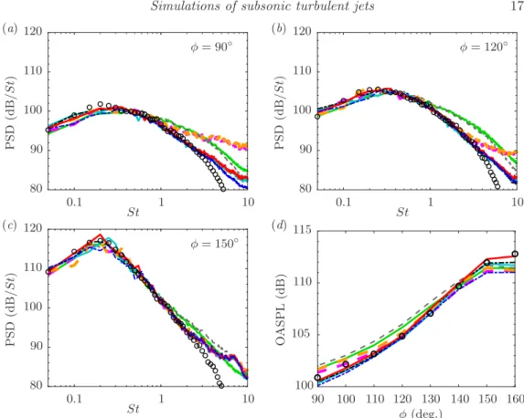
3.2. Effects of nozzle-interior turbulence modelling on far-field acoustic results Figure 9 compares power spectral density (PSD) of pressure fluctuations and overall sound pressure level (OASPL) between experiment and LES cases with and without nozzle-interior turbulence modelling. The PSD is computed with Welch method (block size of 2048, 75% overlap), bin-averaged (bin size ∆St= 0.05) and reported in dB/St, following the same non-dimensionalization as the experiment (see Appendix B). Simi-lar to the direct computation of spectra discussed in_§3.1.4, the FW-H predictions are performed for 36 equally-spaced microphones distributed along the azimuthal angle, and the resulting spectra are azimuthally averaged. The same procedure is applied for

calcu-P S D (d B / S t ) St 0.1 1 10 80 90 100 110 120 (a) φ= 90◦ P S D (d B / S t ) St 0.1 1 10 80 90 100 110 120 (b) φ= 120◦ P S D (d B / S t ) St 0.1 1 10 80 90 100 110 120 (c) φ= 150◦ O A S P L (d B ) φ(deg.) 90 100 110 120 130 140 150 160 100 105 110 115 (d)

Figure 9. (Colour online) Power spectra density of pressure on the polar microphone array at 50D from the nozzle exit (a-c) at various angles φ and (d) overall sound pressure levels: experiment (◦ ), baseline LES10M( ) and64M ( ), and LES with nozzle-interior turbulence modelling BL16M( ), BL16M Turb2 ( ), BL16M Turb( ), BL16M WM

( ),BL16M WM Turb2( ) andBL16M WM Turb( ).

lation of the OASPL in dB, where the frequency range considered for the integration is 0.056St63. To evaluate uncertainty in the experimental noise data, basic techniques were used to estimate the errors due to the microphone sensitivity, statistical errors and errors associated with measurement repeatability. The latter was found to be the main source of uncertainty, in general less than 0.5 dB.

For the baseline cases10M_and64M_{, the noise spectra are reasonably well captured up to} St_≈1. For higher frequencies however, the noise levels from these simulations are over-predicted by the same amount for both grids, indicating that refinement in the jet plume will not reduce the discrepancy. This is observed for sideline angles 90◦

6 φ 6 120◦

, where the large-scale mixing noise is less dominant. For shallow angles to the jet axis, e.g. φ= 150◦

, this high-frequency over-prediction is less severe but the peak radiation around St = 0.2 is now under-predicted. These trends translate into discrepancies of approximately 1.5 to 2 dB in the OASPL, with over-prediction at sideline angles and under-prediction aft.

With nozzle-interior turbulence modelling, the over-prediction observed at high fre-quencies is eliminated, with the notable exception of the case with high amplitude syn-thetic turbulence (i.e., suffixTurb2_{). For these cases, there is an evident change of slope}

and excess high-frequency noise forSt >2 particularly visible at sideline angles, which is likely related to the increase in pressure fluctuations and core-turbulence levels inside the

18 G. A. Br`es et al.

nozzle, as previously discussed. The same trends have been reported in the experimental study by Zaman (2012) where larger spectra amplitudes were observed with the appli-cation of turbulence-generating grids. In the experiment, the increase was also generally more pronounced at 90◦

and higher frequencies.

Aside from these two cases, good agreement with experimental measurements is ob-tained for the present mesh, which is of modest size, at all angles and frequencies up to St_≈2₋3, consistent with the estimate from the grid design. The resulting OASPL directivity curve in figure 9(d) now generally lies within experimental uncer-tainty, with less than 1 dB difference for most angles. The discrepancies appears to be mostly due to the variations in low frequencies related to the relatively short simulation time (see statistical convergence and grid resolution study in _§4.1). Like the flow field results discussed in the previous section, it was found that the grid adaptation has the most significant impact on far-field noise predictions, while the low amplitude synthetic turbulence and wall model have more subtle effects. With the exception of the two LES cases with high input turbulence, the spectra do not contain discernible tones nor visi-ble numerical artifacts that could be directly related to the added modelling inside the nozzle.

4. Laminar versus turbulent jets

4.1. Database validation: statistical convergence and grid resolution study Based on the results presented above, the turbulent case BL16M WM Turb and lami-nar case 10M were selected for further analysis and comparisons. The total simulation time in both cases was increased to tsimc∞/D = 2000. Finally, to investigate grid

con-vergence, an additional simulation for the same configuration and numerical setup than BL16M WM Turb was performed on the refined mesh, the i.e., 69 million cvs grid with double the resolution in the jet plume (see table 1).

4.1.1. Jet plume statistics

Figure 10 shows comparisons of the streamwise velocity statistics in the jet plume between PIV and LES for the extended simulations. The corresponding centerline and lipline profiles are presented in figure 11.As discussed in Appendix A, reliable PIV measurements are not available for x/D <1 because of edge effects near the nozzle.

Despite the significant differences in grid resolution in the jet plume, both simulations

BL16M WM Turb_andBL69M WM Turb_{with nozzle-interior turbulence modelling give similar}

flow-field results, both in good agreement with the experimental measurements. Com-pared to the profiles in figure 7 with statistics computed over 600 acoustic time units (i.e., the duration from the preliminary study), the predictions for the extended simulations show improvements in the statistical convergence. The mesh refinement in the jet plume for caseBL69M WM Turb_{also provided some improvements of the artifacts associated with}

transitions in mesh resolution. As mentioned in §3.1, the discontinuities in RMS levels observed atx/D≈0.5, 2.1 and 5 in figures 10(b) and 11(b) correspond to unstructured grid transitions. With smaller changes in grid spacing on the refined mesh, the grid im-print on RMS levels is reduced in the refined case. For both extended simulations with nozzle-interior turbulence modelling, the length of the potential corexc is well predicted (see table 3). As expected, grid refinement in the jet plume tends to increase the value ofxcand shift the centerline peak RMS fluctuations further downstream. Likewise, after the end of the potential core, the refined case tends to display slightly higher mean and

P IV 0 2 −2 0 10 20 y / D ux/Uj (a) 0 1 0 2 −2 0 10 20 p u′ xu′x/Uj (b) 0 0.16 1 0 M 0 2 −2 0 10 20 y / D 0 2 −2 0 10 20 B L 1 6 M W M T u r b 0 2 −2 0 10 20 y / D 0 2 −2 0 10 20 B L 6 9 M W M T u r b 0 2 −2 0 10 20 y / D x/D 0 2 −2 0 10 20 x/D

Figure 10. (Colour online) Contours of (a) mean and (b) RMS streamwise velocity in the mid-section plane (z= 0): experimental PIV (top row), extended baseline LES10Mand extended LES with nozzle-interior turbulence modellingBL16M WM TurbandBL69M WM Turb.

ux / Uj x/D 0 5 10 15 20 0.2 0.4 0.6 0.8 1.0 (a) centerline lipline p u ′u_x ′/_x Uj x/D 0 5 10 15 20 0 0.05 0.1 0.15 0.2 (b) centerline lipline

Figure 11.(Colour online) Centerline and lipline profiles of (a) mean and (b) RMS streamwise velocity: experiment ( hot-wire,◦ PIV), extended baseline LES10M( ) and extended LES with nozzle-interior turbulence modellingBL16M WM Turb( ) andBL69M WM Turb( ).

RMS values than the standard case, as the increase in resolution in that region leads to prediction improvements of the turbulent mixing.

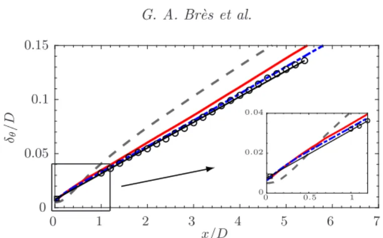
20 G. A. Br`es et al. δθ / D x/D 0 0.05 0.1 0.15 0 1 2 3 4 5 6 7 0 0.02 0.04 0 0.5 1

Figure 12.(Colour online) Profiles of the shear-layer momentum thicknessδθ: experiment ( hot-wire,◦ PIV, linear interpolation), extended baseline LES10M( ) and extended LES with nozzle-interior turbulence modelling BL16M WM Turb ( ) and BL69M WM Turb

( ).

4.1.2. Nozzle-exit conditions and shear-layer development

The shear-layer momentum thicknessδθ are presented in figure 12. Similarly to Bogey & Bailly (2010),δθ is estimated as

δθ(x) = Z r0.05 0 ux(x, r) ux(x,0) 1₋ux(x, r) ux(x,0) dr, (4.1)

where ux is the time- and azimuthal-averaged streamwise velocity. The integral ra-dial bound r0.05 accounts for the slow coflow and corresponds to the distance where

ux(x, r0.05)−U∞= 0.05ux(x,0). The same approach is used to estimate the displacement thicknessδ∗

. Table 3 summarizes all the nozzle-exit boundary layer properties predicted from simulations and estimated from the experimental PIV using linear extrapolation to

x/D= 0. As the shape factorH=δ∗

/δθvaries from 2.59 for fully laminar flow to approx-imately 1.4 for fully turbulent flow (Schlichting & Gertsen 2000), the results confirm the initially laminar and turbulent state of the jets for the different LES. Here the estimated momentum thickness is also comparable to the valuesδθ/D≈0.0055 to 0.0213 reported in the recent experiments by Fontaineet al.(2015) with similar convergent-straight noz-zles and operating conditions.

Figures 13 and 14 shows the evolution of the mean streamwise velocity and streamwise turbulence intensity at different axial locations upstream and downstream of the nozzle exit.As previously discussed, both LES casesBL16M WM Turb

andBL69M WM Turb_{have the same adapted mesh inside the nozzle and the same synthetic}

turbulence and wall modelling applied to the nozzle internal walls. This leads to identical profiles for x/D <0 and similar integral quantities for the nozzle-exit boundary layer. The only noticeable difference is at x/D = 0.04 in figure 14(a) for the maximum RMS levels aroundr/D= 0.5, where the additional resolution in the jet plume for the refined case is better suited to resolve the strong velocity gradients and sharp peak of the RMS levels at the lipline. That peak is missed in the measurement because of limited spa-tial resolution. For both simulations, the linear growth of the shear-layer starts almost immediately at the nozzle exit and closely matches the experimental value in figure 12.

In contrast, for the initially laminar jet in simulation 10M_{, the jet flow development}

is characterized by different features in three distinct regions. Inside the nozzle, the boundary layer is laminar and the jet remains laminar with limited spreading close to the nozzle exit, up tox/D_≈0.2 (see insert in figure 12). This is followed by a rapid growth

r/ D 0.3 0.4 0.5 0.6 0 1 (a) x/D=−0.5 nozzle 0.3 0.4 0.5 0.6 0 1 x/D=−0.05 nozzle 0.3 0.4 0.5 0.6 0 1 x/D= 0.04 0.3 0.4 0.5 0.6 0 1 x/D= 0.5 ux/Uj r/ D 0 0.5 1 0 1 (b) x/D= 1 ux/Uj 0 0.5 1 0 1 x/D= 5 ux/Uj 0 0.5 1 0 1 x/D= 10 ux/Uj 0 0.5 1 0 1 x/D= 15

Figure 13. (Colour online) Profiles of the mean streamwise velocity (a) in the near-nozzle region and (b) in the jet plume: experiment ( hot-wire,◦ PIV), extended baseline LES 10M

( ) and extended LES with nozzle-interior turbulence modellingBL16M WM Turb_{( )}

andBL69M WM Turb_{( ).} r/ D 0.3 0.4 0.5 0.6 0 0.2 (a) x/D=−0.5 nozzle 0.3 0.4 0.5 0.6 0 0.2 x/D=−0.05 nozzle 0.3 0.4 0.5 0.6 0 0.2 x/D= 0.04 0.3 0.4 0.5 0.6 0 0.2 x/D= 0.5 p u′ xu′x/Uj r/ D 0 0.5 1 0 0.2 (b) x/D= 1 p u′ xu′x/Uj 0 0.5 1 0 0.2 x/D= 5 p u′ xu′x/Uj 0 0.5 1 0 0.2 x/D= 10 p u′ xu′x/Uj 0 0.5 1 0 0.2 x/D= 15

Figure 14. (Colour online) Profiles of the RMS streamwise velocity (a) in the near-nozzle region and (b) in the jet plume: experiment ( hot-wire,◦ PIV), extended baseline LES 10M

( ) and extended LES with nozzle-interior turbulence modellingBL16M WM Turb( ) andBL69M WM Turb( ).

22 G. A. Br`es et al. Approach Methodology xc/D δθ/D δ ∗ /D δ99 /D H Experiment PIV 7.5 0.0077 0.012 0.080 1.56 Baseline LES 10M 6.5 0.0051 0.013 0.039 2.54

LES with modelling BL16M WM Turb_{BL69M WM Turb} 7.3_7.7 0.0071_0.0066 0.011_0.010 0.073_0.073 1.55_1.51 Table 3.Estimates of the jet potential core lengthxc, nozzle-exit boundary-layer momentum

thicknessδθ, displacement thicknessδ

∗

, thicknessδ99

and shape factorH.

related to the shear-layer laminar-to-turbulent transition, as indicated by the overshoot of the velocity RMS aroundx/D = 0.5 in figure 11 and figure 14(a). This process then leads to enhanced mixing further downstream, resulting in the larger spreading rate observed in figure 12 and earlier termination of the potential core. Overall, the trends for the potential core length and shear-layer growth are consistent with the results reported by Bogey & Bailly (2010) for simulations of initially laminar jets at Mach 0.9.

4.1.3. Far-field acoustics

In addition to the single microphone in the far field, pressure measurements were also made using a 18-microphone azimuthal ring array whose axial position was varied in order to map the sound field on a cylindrical surface of radius r/D= 14.3 centered on the jet axis. This microphone ring is also used to perform the azimuthal decomposition of the radiated noise discussed in_§4.2. The complete comparison with the LES predictions is presented in figure 15 for all microphones, with the corresponding overall sound pressure level directivity (OASPL) shown in figure 16.

First, for the initially laminar jet, the results of the extended simulation10M_confirms

the conclusion of the preliminary study: the noise spectra are reasonably well predicted for most angles up to frequencySt ≈1, with over-prediction at higher frequencies and slight under-prediction of the peak radiation around St = 0.2. The discrepancies are more pronounced on the cylindrical microphone array (see zoomed-in view of the spectra in figure 18) and lead to the mismatch in shape for the noise directivity observed in the OASPL levels in figure 16. Experimental studies by Brown & Bridges (2006), Zaman (2012), and Karon & Ahuja (2013) all reported similar increased levels at high frequencies for subsonic jets with (nominally) laminar initial shear layers, compared to jets with (nominally) turbulent ones. In particular, Brown & Bridges (2006) applied a thin wrap of reticulated foam metal (RFM) inside their nozzle to trip the boundary layer, similar to the carborundum strip used in the present experiments. The RFM inserts changed the characteristics of the nozzle-exit boundary layer from laminar to turbulent and eliminated the high frequency noise.

For the initially turbulent jets, there is little variation between the results from the standard and refined simulations, for most angles and relevant frequencies. With the ex-tended simulation time, the low frequency part of the spectra shows better convergence compared to the preliminary results in figure 9 and the predictions are further improved, now typically within 0.5 dB of the measurements. The main discernible differences be-tween the spectra from the two LES are observed in the grid cut-off frequency for the high anglesφ>150◦

: at these angles, the limit frequency is aboutSt_≈2 for the stan-dard case BL16M WM Turb _{and St ≈ 4 for the refined case} BL69M WM Turb _{with double}

the resolution in the jet plume. Here, it is important to note that these discrepancies are outside of the main frequency range of interest and with levels 25 to 30 dB lower that the peak radiated noise, such that they do not significantly impact the predictive

P S D (d B / S t ) St 0.1 1 10 40 dB 100 100 100 100 100 100 100 100 100 φ= 90◦ φ= 120◦ φ= 140◦ φ= 150◦ φ= 160◦ φ= 105◦ φ= 135◦ φ= 145◦ φ= 155◦ (a) St 0.1 1 10 40 dB 100 100 100 100 100 100 100 100 φ= 90◦ φ= 100◦ φ= 110◦ φ= 120◦ φ= 130◦ φ= 140◦ φ= 150◦ φ= 160◦ (b)

Figure 15.(Colour online) Power spectra density of pressure (a) on the cylindrical microphone array of radiusr= 14.3Dand (b) on the polar microphone array at 50Dfrom the nozzle exit for the different anglesφ: experiment (◦), extended baseline LES10M( ) and extended LES with nozzle-interior turbulence modellingBL16M WM Turb( ) andBL69M WM Turb( ).

24 G. A. Br`es et al. O A S P L (d B ) φ(deg.) 105 110 115 120 90 100 110 120 130 140 150 160 (a) φ(deg.) 100 105 110 115 90 100 110 120 130 140 150 160 (b)

Figure 16.(Colour online) Overall sound pressure level directivity (a) on the cylindrical micro-phone array of radiusr= 14.3D and (b) on the polar microphone array at 50Dfrom the nozzle exit: experiment (◦), extended baseline LES10M( ) and extended LES with nozzle-interior turbulence modellingBL16M WM Turb( ) andBL69M WM Turb( ).

capabilities nor use of the database for sound-source modelling. Overall, the statistical convergence and grid resolution studies provide thorough validation and confidence in the LES database of caseBL16M WM Turb_{, for flow and noise data up to St≈2−3. All}

of the remaining analysis is therefore conducted using that longer database. 4.1.4. Near-field acoustics

For the eduction of wavepacket signatures and further investigation of the tones ob-served in the LES spectra inside the nozzle, the experiment was also instrumented with a 48-microphone cage array consisting in 6 azimuthally equispaced microphones at 7 dif-ferent locations in the near field on the jet. Figure 17 shows the comparison with the LES predictions at three representative locations: (x/D, r/D) = (0.12,0.72), (b) (2.00,0.91) and (c) (4.47,1.33).

For the microphone ring closest to the nozzle exit, corresponding to a jet inlet angle of φ _≈99.5◦

, the discrete tones associated with the resonant acoustic waves are again observed in the spectra, consistent with the results inside the nozzle discussed in sec-tion §3.1.4. For both simulations with initially turbulent jet, the shape of the spectra and the frequency and amplitude of the tones closely match the experimental measure-ments. For the simulation with initially laminar jet, the tones are still present at the same frequencies but the overall levels are higher because of the enhanced noise radia-tion related to the shear-layer laminar-to-turbulent transiradia-tion. Addiradia-tional analysis of the discrete tones is presented in Appendix C.

For the near-field microphones further downstream, the same conclusions hold in terms of agreement with experiment for the simulations with initially turbulent jet and over-predictions for the simulation with initially laminar jet. At these locations corresponding to the peak radiation angles (i.e., φ_≈153.9◦

and 163.4◦

), the spectra levels are much higher and there is no visible tonal component. As discussed in detail in the work of Towne et al.(2017) and Schmidt et al. (2017), the resonant acoustic waves are trapped within the potential core of the jet and decay rapidly away from the jet. Therefore, there are no discernible tones in figure 17 (b) and (c), nor in figure 15 for the far-field noise predictions.

4.2. Azimuthal mode decomposition of the radiated noise

Dating back to Michalke & Fuchs (1975), who first argued that low-order azimuthal modes would be the dominant sources of sound in subsonic circular jets, many

experi-P S D (d B / S t) 0.1 _St 1 150 140 130 120 (a) 0.1 _St 1 150 140 130 120 (b) 0.1 _St 1 150 140 130 120 (c)

Figure 17.(Colour online) Power spectra density of pressure on the near-field cage microphone array at (a) (x/D, r/D) = (0.12,0.72), (b) (2.00,0.91) and (c) (4.47,1.33): experiment ( ◦), extended baseline LES10M( ) and extended LES with nozzle-interior turbulence modelling

BL16M WM Turb( ) andBL69M WM Turb( ). The arrows indicate the frequencies of the trapped acoustic waves (see Appendix C).

mental jet studies have suggested that low-frequency noise (i.e., Strouhal numberSt <1) may be decomposed into just 3 Fourier azimuthal mode m = 0, 1 and 2 (Juv´e et al. 1979; Kopiev et al. 2010; Cavalieri et al. 2011, 2012, amongst others). The azimuthal mode analysis is applied to the present experimental and LES databases and extended to higher frequencies, to further investigate the differences observed in radiated noise between jets with laminar and turbulent nozzle-exit boundary layer state. For both ex-periment and simulation, the azimuthal decomposition is performed using the data from 18 microphones evenly-spaced in the azimuthal direction, on the cylindrical array of ra-dius 14.3D, following the procedure described by Cavalieriet al.(2012). The output is the complex acoustic pressure as a function of frequency and azimuthal modemat each jet inlet angle on the array. The procedure was reproduced using the LES data from 128 evenly-spaced microphones instead of 18, and provided similar results and conclusions for the azimuthal modes and frequency range considered.

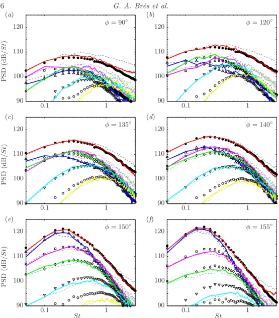
Figure 18 shows the experimental and numerical spectra of the total signal and the first five azimuthal modes for a few representative jet inlet angles φ. In addition, PSD levels from the different modes at selected frequencies are plotted as a function of φin figure 19. In these figures, the total noise spectra from experiment (black solid circle), LES cases10M _{(dashed grey line) and} BL16M WM Turb_{(solid red line) is the same data}

reported in figure 15(a).

For the initially turbulent jet, the agreement between measurement and LES is again excellent, particularly for the first four modes. Figure 19(a-c) shows the PSD values from figure 18 extracted at specific low frequenciesSt= 0.1, 0.2 and 0.3. In the low frequency range 0.05 6 St 6 0.4, the axisymmetric azimuthal mode m = 0 is dominant at the peak radiation anglesφ = 140◦

−160◦

, followed by mode m = 1 and thenm = 2. At the lower inlet angles φ 6135◦

, the mode order (in terms of importance) tends to be reversed, with modem= 1 and 2 more energetic thanm= 0, and the differences are less pronounced. Furthermore, the higher-order modesm>3 have much lower contributions. These results are confirmed by the OASPL curves computed over the full frequency range 0.056St63 in figures 20(a) and (b). In these figures, the total OASPL is compared to that calculated with selected azimuthal modes retained for the pressure, namely either modem= 0 only, modesm= 0 to 1, etc ... up to modesm= 0 to 4. Atφ= 160◦

, mode m=0 contributes to OASPLm/OASPLtotal= 86% of the total acoustic energy, and this value goes to more than 99.2% when the first 3 modes are considered. Over all angles, the first 3 Fourier azimuthal modes of the LES data recover more than 65% of the total acoustic energy, which means that a prediction based on these 3 dominant modes would

26 G. A. Br`es et al. P S D (d B / S t ) 0.1 1 90 100 110 120 (a) φ= 90◦ 0.1 1 90 100 110 120 (b) φ= 120◦ P S D (d B / S t ) 0.1 1 90 100 110 120 (c) φ= 135◦ 0.1 1 90 100 110 120 (d) φ= 140◦ P S D (d B / S t ) St 0.1 1 90 100 110 120 (e) φ= 150◦ St 0.1 1 90 100 110 120 (f) φ= 155◦

Figure 18.(Colour online) Azimuthal mode decomposition of the radiated noise at specific an-glesφfor the experimental data (symbols), initially laminar jet10M_{(dashed lines) and turbulent}

jetBL16M WM Turb_{(solid lines): (}•, ) total (i.e., all modes); (△ _{, ) modem= 0;} (, )m= 1; (⋄, )m= 2; (∇, )m= 3; (◦, )m= 4.

be within 1.9dB of the total OASPL value. These results are all consistent with the experimental trend previously reported in the literature. At higher frequencies, the PSD levels are lower and more modes have comparable contributions to the radiated sound (see figure 19(d-f)).

For the initially laminar jet, the same conclusions hold, despite the significant differ-ences in noise levels previously discussed. In the low frequency rangeSt <1 where the radiation from the laminar and turbulent jets are similar, the azimuthal mode decom-position for the LES case10M _{provides results similar to those of the turbulent jet. In}

the higher frequency range, the low azimuthal modes have elevated levels compared to the turbulent case (see figure 19(e-f)). However, these discrepancies appear to be directly