Sensitivity of Swept-Wing, Boundary-Layer Transition to Spanwise-Periodic Discrete Roughness Elements

SENSITIVITY OF SWEPT-WING, BOUNDARY-LAYER TRANSITION TO SPANWISE-PERIODIC DISCRETE ROUGHNESS ELEMENTS

A Thesis by

DAVID EDWARD WEST

Submitted to the Office of Graduate and Professional Studies of Texas A&M University

in partial fulfillment of the requirements for the degree of MASTER OF SCIENCE

Chair of Committee, William S. Saric Committee Members, Helen L. Reed

David A. Staack

Head of Department, Rodney D. W. Bowersox

December 2014

Major Subject: Aerospace Engineering

ii ABSTRACT

Micron-sized, spanwise-periodic, discrete roughness elements (DREs) were applied to and tested on a 30° swept-wing model in order to study their effects on boundary-layer transition in flight where stationary crossflow waves are the dominant instability. Significant improvements have been made to previous flight experiments in order to more reliably determine and control the model angle of attack (AoA) and unit Reynolds number (Re′). These improvements will aid in determining the influence that DREs have on swept-wing, laminar-turbulent transition. Two interchangeable leading-edge surface-roughness configurations were tested: polished and painted. The baseline transition location for the painted leading edge (increased surface roughness) was unexpectedly farther aft than the polished. Transport unit Reynolds numbers were achieved using a Cessna O-2A Skymaster. Infrared thermography, coupled with a post-processing code, was used to globally extract a quantitative boundary-layer transition location. Each DRE configuration was compared to curve-fitted baseline data in order to determine increases or decreases in percent laminar flow while accounting for the influence of small differences in Re' and

AoA. Linear Stability Theory (LST) guided the DRE configuration test matrix. In total, 63 flights were completed, where only 30 of those flights resulted in useable data. While the results of this research have not reliably confirmed the use of DREs as a viable laminar flow control technique in the flight environment, it has become clear that significant computational studies, specifically direct numerical simulation (DNS) of these particular

iii

DRE configurations and flight conditions, are a necessity in order to better understand the influence that DREs have on laminar-turbulent transition.

iv DEDICATION

This work is dedicated to my wife and best friend, Rebecca. Her continual support, optimism, and love have helped me endeavor through my education with a sense of determination and enthusiasm.

v

ACKNOWLEDGEMENTS

This research effort was the culmination of several contributors through funding, advisement, corroboration, motivation, and encouragement. It is because of these people and their contributions that this research was possible. Funding for this effort was provided by the National Aeronautics and Space Administration (NASA) through Analytical Mechanics Associates, Inc. (AMA-Inc) and by Air Force Research Laboratories (AFRL) at Wright-Patterson Air Force Base (WPAFB) through General Dynamics IT.

I would first like to thank Dr. William Saric for providing me the opportunity, advisement and encouragement needed to accomplish this research effort. Before I entered graduate school at Texas A&M University, Dr. Saric brought me on as an undergraduate research assistant at the Klebanoff-Saric Wind Tunnel (KSWT), where my interest in research was first cultivated and developed. Upon graduation, I was afforded the opportunity to work at the Flight Research Lab as an engineering associate, where my desire to pursue a graduate degree really took hold. Now, looking back, I’m greatly appreciative for the four-plus years of guidance and wisdom that Dr. Saric provided me. I know that laminar flow control using DREs has been a passion and investment for Dr. Saric, and I am honored to be a small part of the research process. I don’t take lightly the trust that he put in me to conduct a worthwhile experiment. I would also like to thank my graduate committee members (both current and former) Dr. Helen Reed, Dr. David Staack and Dr. Devesh Ranjan for their guidance and support throughout this research endeavor. They were always willing to assist when needed and offer suggestions for the success of

vi

my work. I’d also like to thank our program specialists Colleen Leatherman and Rebecca Mariano for their logistical support of both my research and that of the Aerospace Engineering Department. Without their experience and willingness to exceed expectations, our research team would never come close to the efficiency and productivity it now enjoys.

While completing this research, I had the opportunity to work with several graduate and undergraduate students who contributed so much to the success of this effort. Most of all, I would like to thank Brian Crawford and Dr. Tom Duncan. These two extremely dedicated and hard-working colleagues have supported me throughout my entire graduate career at Texas A&M. Without their skills, experience and expertise, this research would never have had the amount of quality, sophistication and attention to detail it needed to be successful. From model design, instrumentation development, data acquisition & processing, and flight crew support, these young men have truly shown their dedication to research and to myself. I wholeheartedly consider them more than just colleagues or class-mates, but as genuinely devoted friends. Additionally, Matthew Tufts provided all of the computational support for this research effort and also showed me continual support and friendship. Every good experiment has a computational counterpart, and his was exemplary. I would also like to acknowledge the following former students who helped develop my skills as a researcher throughout my undergraduate and graduate career: Dr. Lauren Hunt, Dr. Rob Downs and Dr. Matthew Kuester. Also, I would like to acknowledge the following students (both former and current) for their support of this research by assisting with flight crew duties of co-pilot and ground crew: Dr. Jacob

vii

Cooper, Colin Cox, Alex Craig, Brian Crawford, Dr. Rob Downs, Dr. Tom Duncan, Kristin Ehrhardt, Dr. Bobby Ehrmann, Joshua Fanning, Simon Hedderman, Kevin Hernandez, Heather Kostak, Dr. Matthew Kuester, Erica Lovig, Dr. Chi Mai, Ian Neel, Matthew Tufts, and Thomas Williams.

The test pilots who contributed to this research include both Lee Denham and Lt Col Aaron Tucker PhD. I would like to thank both of them for their talent, continual dedication and expertise which helped make these experiments both safe and successful. They were always available for early mornings and made it a point to bring a professional and accommodating attitude to every flight. Additionally, these experiments would not be possible without the diligence and proficiency of our A&P mechanic Cecil Rhodes. Cecil continually and reliably maintained the aircraft to ensure the safety of every flight. Moreover, he provided extensive knowledge and training for myself and other students in the areas of mechanics, sheet metal work, woodworking, milling and painting.

Finally, I would like to thank my family for their perpetual support and prayers throughout my career as a student. I thank my parents, Jim and Linda West, who always encouraged me to do my best and to be proud of my accomplishments; without them, I would not have been able to call myself a proud Aggie. I’d also like to thank my wife, Rebecca, to whom this work is dedicated and who was and is always there for me.

viii

NOMENCLATURE

5HP five-hole probe

A total disturbance amplitude

Ao reference total disturbance amplitude, baseline at x/c = 0.05

AMA-Inc Analytical Mechanics Associates, Inc.

AoA angle of attack

ASU Arizona State University BCF baseline curve fit

c chord length, 1.372 m

Cp,3D coefficient of pressure

CO Carbon Monoxide

DAQ data acquisition

DBD dielectric-barrier discharge DFRC Dryden Flight Research Center DNS direct numerical simulation

DREs spanwise-periodic discrete roughness elements DTC digital temperature compensation

FRL Flight Research Laboratory (Texas A&M University) FTE flight-test engineer

GTOW gross take-off weight

ix

IR infrared

k step height, forward-facing (+), aft-facing (-) KIAS knots indicated airspeed

KSWT Klebanoff-Saric Wind Tunnel (Texas A&M University) LabVIEW Laboratory Virtual Instrument Engineering Workbench

(data acquisition software)

LE leading edge

LFC laminar flow control

LIDAR Light Detection And Ranging LST Linear Stability Theory

M Mach number

MSL mean sea level

N experimental amplification factor (natural log amplitude ratio from LST)

Neff Effective N-Factor (depends on DRE x/c placement) Nmax maximum N-Factor possible for specific wavelength Ntr transition N-Factor (N at x/c transition location)

NASA National Aeronautics and Space Administration NPSE Nonlinear Parabolized Stability Equation

NTS non-test surface

x

ONERA Office National d'Études et de Recherches Aérospatiales (French aerospace research center)

P2P Pixels 2 Press (DRE manufacturing company) PDF probability density function

PID proportional integral derivative (a type of controller)

Pk-Pk peak-to-peak

PSD power spectral density

ps freestream static pressure

q dynamic pressure

Reʹ unit Reynolds number

Rec chord Reynolds number

Reθ,AL attachment-line momentum-thickness Reynolds number

RMS root mean square

RMSE root mean square error

RTD resistance temperature detector RTV room temperature vulcanizing

s span length of test article, 1.067 m S3F Surface Stress Sensitive Film

std standard deviation of the measurement

SWIFT Swept-Wing In-Flight Testing (test-article acronym)

SWIFTER Swept-Wing In-Flight Testing Excrescence Research (test-article acronym)

xi

T temperature

TAMU-FRL Texas A&M University Flight Research Laboratory TEC thermoelectric cooler

TLP traversing laser profilometer TRL technology readiness level

T-S Tollmien-Schlichting, boundary-layer instability

Tu freestream turbulence intensity

U∞ freestream velocity

VFR visual flight rules

VI virtual instrument (LabVIEW file) WPAFB Wright-Patterson Air Force Base

x, y, z model-fixed coordinates: leading-edge normal, wall-normal,

leading-edge-parallel root to tip

xt, yt, zt tangential coordinates to inviscid streamline

X, Y, Z aircraft coordinates: roll axis (towards nose), pitch axis (towards

starboard), yaw axis (towards bottom of aircraft)

xtr,DRE streamwise transition location with DREs applied

xtr,baseline streamwise transition location of the baseline (no DREs)

α model angle of attack

αoffset chord-line angle offset (5HP relative to test article)

β aircraft sideslip angle

xii

δ99 boundary-layer thickness at which u/Uedge = 0.99 ΔLF% percent-change in laminar flow

θ boundary-layer momentum thickness

θAC pitch angle of aircraft

θAC,offset aircraft-pitch angle offset (5HP relative to test article)

𝜆 wavelength

Λ leading-edge sweep angle

σBCF baseline curve fit uncertainty

xiii TABLE OF CONTENTS Page ABSTRACT ... ii DEDICATION ...iv ACKNOWLEDGEMENTS ... v NOMENCLATURE ... viii

TABLE OF CONTENTS ... xiii

LIST OF FIGURES ... xv

LIST OF TABLES ... xviii

1. INTRODUCTION ... 1

1.1 Motivation ... 1

1.2 Swept-Wing Boundary-Layer Stability and Transition ... 3

1.3 Previous Experiments ... 10

1.4 Experimental Objectives ... 13

2. IMPROVEMENTS TO PREVIOUS TAMU-FRL DRE EXPERIMENTS ... 15

2.1 Flight Research Laboratory ... 15

2.2 Overview and Comparison of SWIFT and SWIFTER ... 19

2.3 Five-Hole Probe and Calibration ... 23

2.4 Infrared Thermography ... 28

2.5 Traversing Laser Profilometer ... 39

3. EXPERIMENTAL CONFIGURATION AND PROCEDURES ... 42

3.1 Experimental Set-up, Test Procedures and Flight Profile ... 42

3.2 Surface Roughness ... 48

3.3 Linear Stability Theory ... 55

3.4 Spanwise-Periodic Discrete Roughness Elements ... 57

4. RESULTS ... 64

4.1 Infrared Thermography Transition Data ... 65

4.2 Baseline Curve Fit ... 68

xiv

5. SUMMARY, CONCLUSIONS, AND RECOMMENDATIONS ... 84

5.1 Flight-Test Summary ... 84

5.2 Future Research Recommendations ... 85

REFERENCES ... 88

APPENDIX A PERCENT LAMINAR FLOW FIGURES ... 94

APPENDIX B SWIFTER OML AND COEFFICIENT OF PRESSURE DATA ... 116

xv LIST OF FIGURES

Page Fig. 1 Transition paths from receptivity to breakdown and turbulence

(modified figure from Saric et al. 2002 [4]) ... 4

Fig. 2 Inviscid streamline for flow over a swept wing ... 6

Fig. 3 Crossflow boundary-layer profile (Saric et al. 2003 [10]) ... 6

Fig. 4 Crossflow streaking observed through naphthalene flow visualization ... 8

Fig. 5 Co-rotating crossflow vortices ... 8

Fig. 6 Raw infrared thermography image of a saw-tooth crossflow transition front ... 10

Fig. 7 Stemme S10-V (left) and Cessna O-2A Skymaster (right) hangared at TAMU-FRL ... 16

Fig. 8 Dimensioned and detailed three-view drawing of the Cessna O-2A Skymaster ... 18

Fig. 9 SWIFTER and hotwire sting mount attached to the port and starboard wings of the Cessna O-2A Skymaster respectively (Photo Credit: Jarrod Wilkening) ... 20

Fig. 10 SWIFT (left) & SWIFTER (right) side-by-side ... 21

Fig. 11 SWIFTER airfoil graphic (top) and LE actuation system (bottom) (modified figure from Duncan 2014 [32]) ... 23

Fig. 12 Five-hole probe (5HP): freestream static ring (left), conical tip (middle), pressure port schematic (right) ... 24

Fig. 13 SWIFT five-hole probe mount ... 25

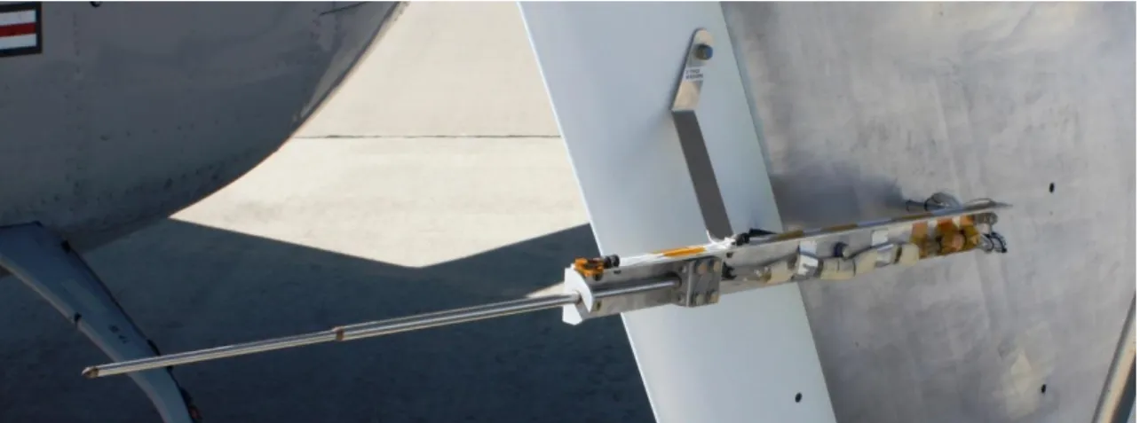
Fig. 14 SWIFTER five-hole probe mount ... 26

Fig. 15 Temperature controlled pressure transducer box ... 27

Fig. 16 SWIFTER heating sheet layout: Blue heating wire, Red RTV silicone, Insulation and reference RTD not pictured ... 30

xvi

Fig. 17 Idealized graphic of wall heated model (not to scale) (top), Temperature distribution near transition (bottom) (Crawford et al.

2013 [35]) ... 32

Fig. 18 Raw IR image from SWIFT model with qualitative transition front detection at 50% chord. (modified figure from Carpenter (2009) [14]) ... 35

Fig. 19 Raw IR image from SWIFTER model with qualitative transition front detection at 35-40%. ... 35

Fig. 20 Comparison of raw (left) and processed (right) IR images ... 37

Fig. 21 Raw IR image overlaid on SWIFTER model in flight ... 37

Fig. 22 Traversing Laser Profilometer with labeled components (modified figure from Crawford et al. 2014b [37]) ... 41

Fig. 23 SWIFTER and SWIFT ßoffset schematic (angles are exaggerated for visualization purposes) (modified figure from Duncan (2014) [32]) ... 43

Fig. 24 Instrumentation layout in rear of O-2A cabin (Duncan 2014 [32]) ... 44

Fig. 25 Typical flight profile ... 47

Fig. 26 Typical Re′ and α traces while on condtion ... 47

Fig. 27 SWIFT surface roughness spectrogram of painted LE. Data taken using the TLP ... 49

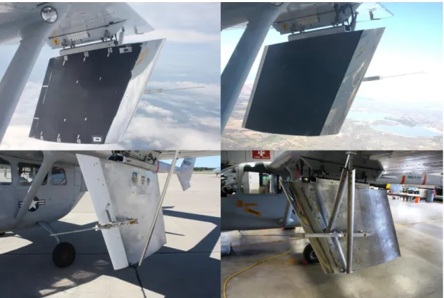
Fig. 28 SWIFTER model in flight with polished (left) and painted (right) LE installed ... 50

Fig. 29 SWIFTER LE being measured with the TLP ... 51

Fig. 30 Wooden LE stand for traversing laser profilometer measurements ... 52

Fig. 31 SWIFTER painted LE spectra for x/c = -0.004 – 0.004 (-0.4 to 0.4 % chord) ... 53

Fig. 32 SWIFTER painted LE spectra for x/c = 0.005 – 0.077 (0.5 to 7.7 % chord) ... 54

Fig. 33 SWIFTER painted LE spectra for x/c = 0.067 – 0.146 (6.7 to 15.0 % chord) ... 54

Fig. 34 N-Factor plot for SWIFTER at α = -6.5° and Re′ = 5.5 x 106/m: The plot on the right is a zoomed in version of the plot on the left. ... 56

xvii

Fig. 36 DRE application photos: constant chord markers (left), DRE &

monofilament alignment (right) ... 60

Fig. 37 Example post-processed IR image ... 66

Fig. 38 Direct IR comparison between baseline flight 862 (left) and DRE flight 863 (right) with target conditions of α = -6.5° & Re′ = 5.70 x 106_{/m. [12µm|2.25mm|1mm|2.30%|02-14] ... 68}

Fig. 39 Baseline-transition surface fit for polished leading edge, ... 69

Fig. 40 Baseline-transition surface fit for painted leading edge, ... 70

Fig. 41 Baseline transition comparison for α = -6.5° ... 71

Fig. 42 Baseline transition comparison for α = -7.5° ... 72

Fig. 43 DRE flight 871 transition comparison for α = -6.5° ... 74

Fig. 44 DRE flight 871 transition comparison for α = -7.5° ... 75

Fig. 45 Direct IR comparison between baseline flight 862 (left) and DRE flight 871 (right) with target conditions of α = -6.5° & Re′ = 5.50 x 106/m. [12µm|2.25mm|1mm|1.10%|11-13] ... 76

Fig. 46 Direct IR comparison between baseline flight 862 (left) and DRE flight 871 (right) with target conditions of α = -7.5° & Re′ = 5.30 x 106/m. [12µm|2.25mm|1mm|1.10%|11-13] ... 77

Fig. 47 DRE flight 847 transition comparison for α = -6.5° ... 78

Fig. 48 DRE flight 847 transition comparison for α = -7.5° ... 79

Fig. 49 DRE flight 870 transition comparison for α = -6.5° ... 79

Fig. 50 DRE flight 870 transition comparison for α = -7.5° ... 80

Fig. 51 DRE flight 829 transition comparison for α = -6.5° ... 81

Fig. 52 DRE flight 829 transition comparison for α = -7.5° ... 81

Fig. 53 DRE flight 840 transition comparison for α = -7.5° ... 82

xviii LIST OF TABLES

Page Table 1 Cessna O-2A Specifications ... 19 Table 2 RMSE and Pk-Pk values of the 5HP calibration (modified table from

Duncan 2014 [32]) ... 28 Table 3 Effective N-Factor Chart for SWIFTER at α = -6.5° & Re′ = 5.5 x

106/m ... 57 Table 4 DRE configurations tested on the polished LE ... 62 Table 5 DRE configurations tested on the painted LE ... 63

1

1. INTRODUCTION

This thesis describes, characterizes, and reviews the experimental research on the feasibility of using spanwise-periodic, discrete roughness elements (DREs) as a reliable and consistent means of swept-wing laminar flow control in the flight environment. These experiments are a continuation of numerous efforts aimed at delaying laminar-turbulent transition at the Texas A&M University Flight Research Laboratory (TAMU-FRL).

This introduction encapsulates the motivation for laminar-flow control, the theory behind transition instabilities, previous experiments showing the development of DREs as a control technique, and finally the objectives this research hopes to achieve. Significant emphasis is placed upon improvements to previous DRE experiments so as to more reliably determine the sensitivity of laminar-turbulent transition to DREs in flight. The experimental methods, procedures, and results are enumerated and documented along with final overview, discussion and summary. Concurrent computational support was provided by Matthew Tufts, a doctoral candidate in the Aerospace Engineering department at Texas A&M University.

1.1Motivation

Enhancing aircraft efficiency is currently, and will continue to be, a top priority for military, commercial, and general aviation. Specifically, aircraft efficiency can be gained by reducing skin friction drag, which for a commercial transport aircraft represents about 50% of the total drag (Arnal & Archambaud 2009 [1]). A viable option for drag reduction

2

is through laminar flow control (LFC) or more specifically the delaying of laminar-turbulent boundary-layer transition. Sustained laminar flow over 50% of a transport aircraft’s wings, tail surfaces, and nacelles could result in an overall drag reduction of 15% (Arnal & Archambaud 2009 [1]). A direct benefit of drag reduction includes lower specific fuel consumption which translates directly into increased range, heavier payloads, or overall lower operating costs.

Controlling laminar-turbulent boundary-layer transition can be accomplished through either active and passive methods or a hybrid of the two. These methods can include suction near the leading edge, reduction of leading edge surface roughness, unsweeping the leading edge to something less than 20º, or even through the use of DREs applied near the attachment line of a swept wing (Saric et al. 2011 [2]). DREs in particular, are aimed at delaying transition by controlling the crossflow instability. Over the course of approximately eighteen years, DREs have been tested in both wind tunnels and in the flight environment at compressibility conditions ranging from subsonic to supersonic. Throughout these experiments, DREs have been implemented in an assortment of ways that vary widely in shape, size, application and operation; however, all variants are intended to serve the same fundamental purpose of controlling crossflow. The three principal types of DREs include: appliqué, pneumatic, and dielectric-barrier discharge (DBD) plasma actuators. Although pneumatic and plasma techniques can have a variable amplitude and distribution, and in principle be active, in this thesis they are considered to be passive.

3

DRE configurations that have successfully delayed laminar-turbulent transition are almost exclusively found in wind tunnel experiments, while the flight environment has achieved only limited success e.g. Saric et al. (2004) [3]. In order to broaden the understanding, implementation and utilization of DREs as a viable LFC technique, it is crucial to both quantify the sensitivity of transition to DREs and to repeatedly demonstrate delayed transition in the flight environment.

1.2Swept-Wing Boundary-Layer Stability and Transition

As stated earlier, DREs are specifically designed to delay boundary-layer transition by controlling the crossflow instability; however, crossflow is not the only instability mechanism that can lead to breakdown and transition to turbulence. Swept wings, in particular, are susceptible to four major instabilities including Tollmien-Schlichting (T-S) (streamwise), crossflow, attachment-line, and Görtler (centrifugal) instabilities. Transition to turbulence can occur through one of these major instabilities because unstable disturbances grow within the boundary layer. In order to focus on controlling only crossflow, the other three instabilities must be suppressed or precluded through airfoil & wing design. Before discussing methods of suppression, it is important to briefly describe the receptivity process and each of the instabilities with a more inclusive focus on crossflow.

Receptivity and Swept-Wing Instabilities

Receptivity is essentially the process through which freestream disturbances enter the boundary layer as steady and/or unsteady fluctuations, which then interact with the surface characteristics of a wing/airfoil. Receptivity establishes the initial conditions of

4

disturbance amplitude, frequency, and phase for the breakdown of laminar flow (Saric et al. 2002 [4]). While there are several paths from receptivity to breakdown and turbulence, as shown in Fig. 1, this research focuses on path A. Path A is the traditional avenue for low disturbance environments, where modal growth is significant and transient growth is insignificant. Morkovin (1969) [5], Morkovin et al. (1994) [6], Saric et al. (2002) [4], and Hunt (2011) [7] provide a more complete description of the process and the different paths to breakdown.

Fig. 1 Transition paths from receptivity to breakdown and turbulence (modified figure from Saric et al. 2002 [4])

The Tollmien-Schlichting instability, colloquially referred to as T-S waves, is a streamwise instability that occurs in two-dimensional flows and at the mid-chord region of swept wings. This instability is driven by viscous effects at the surface and often occurs due to a local suction peak or a decelerating boundary layer. Accelerating pressure

Receptivity

Forcing Environmental Disturbances

Transient Growth Primary Modes Secondary Mechanisms Breakdown Turbulence Bypass increasing amplitude A B C D E

5

gradients are the basis for all natural LFC airfoils that are subject to T-S waves because T-S waves are stabilized by favorable pressure gradients.

Attachment-line instabilities and leading-edge contamination, even though they are different phenomena, are both typically inherent to swept wings. If the boundary layer at the attachment line on a swept wing becomes turbulent, either due to leading-edge radius design or contamination from another source, then the turbulence can propagate along the attachment line and contaminate the boundary layer on both wing surfaces aft of the initial entrained disturbance. It is generally accepted that the solution to this particular instability and contamination is to design your swept wing such that the attachment-line, momentum-thickness Reynolds number, Reθ,AL, is kept below the critical value of approximately 100

(Pfenninger 1977 [8]).

The Görtler instability is a wall-curvature-induced, counter-rotating centrifugal instability that is aligned with the streamlines (Saric 1994 [9]). It is often referred to as a centrifugal instability and is caused by a bounded shear flow over a concave surface. This instability is easily eliminated by avoiding any concave curvature before the pressure minimum on a swept wing.

Finally, the crossflow instability, found in three-dimensional boundary layers, develops as a result of wing sweep coupled with pressure gradient. This coupled interaction between wing sweep and pressure gradient produces curved streamlines at the edge of the boundary layer as depicted in Fig. 2. Inside the boundary layer, the streamwise velocity decreases to zero at the wall, but the pressure gradient remains unchanged. This imbalance of centripetal acceleration and pressure gradient produces a secondary flow that is

6

perpendicular to the inviscid streamline, called the crossflow component. The crossflow component of the 3-D boundary layer must be zero at both the wall and the boundary-layer edge producing an inflection point in the profile. This inflection point is well known to be an instability mechanism. Fig. 3 shows the resultant crossflow boundary-layer profile along with its components.

Fig. 2 Inviscid streamline for flow over a swept wing

Fig. 3 Crossflow boundary-layer profile (Saric et al. 2003 [10])

7

When dealing with the crossflow instability, freestream fluctuations or disturbances are particularly important. Crossflow can develop as either stationary or traveling vortices, which are directly influenced by freestream disturbances. A low freestream-disturbance environment is dominated by stationary crossflow while a high freestream-disturbance environment is dominated by traveling crossflow. Deyhle & Bippes (1996) [11], Bippes (1999) [12], White et al. (2001) [13], and Saric et al. (2003) [10] all provide evidence/explanation of this phenomenon; therefore, it is generally accepted that crossflow in the flight environment (low freestream disturbance) is dominated by stationary crossflow vortices. While both stationary and traveling crossflow exist, transition-to-turbulence is typically the result of one or the other and not both simultaneously. Since this research takes place in the flight environment, it is expected that the crossflow instability is dominated by stationary waves. Previous flight experiments by Carpenter (2010) [14] show little evidence of travelling crossflow waves. All further discussion of crossflow in this thesis will be in reference to the stationary vortices.

Globally, crossflow can be described as a periodic structure of co-rotating vortices whose axes are aligned to within a few degrees of the local inviscid streamlines (Saric et al. 2003 [10]). These periodic vortices can be observed as streaking when employing flow visualization techniques. Fig. 4 is an example of using naphthalene flow visualization to observe the periodic crossflow streaks on a 45° swept wing, where flow is from left to right. When observing traveling crossflow, a uniform streaking pattern would not be apparent due to the nature of the traveling vortices, which would “wash out” any evidence

8

of a periodic structure. Additionally, Fig. 5 shows a graphical representation of the crossflow vortices when viewed by looking downstream. The spacing or wavelength of the crossflow vortices, shown by 𝜆 in Fig. 5, is an extremely important parameter when it comes to LFC through DREs. This wavelength is dependent on and unique to wing geometry and freestream conditions. Each swept wing, that is susceptible to crossflow, will have its own unique spacing of the crossflow instability. More detail on this wavelength will be provided in the Linear Stability Theory section.

Fig. 4 Crossflow streaking observed through naphthalene flow visualization

9

Crossflow-Induced Transition

As mentioned previously, T-S, attachment-line, and Görtler instabilities can all be minimized or eliminated through prudent airfoil design by inducing a favorable pressure gradient as far aft as possible, keeping Reθ,AL below a critical value, and avoiding concavity

in wall curvature before the pressure minimum respectively. Once these instabilities are suppressed, only crossflow remains. It is important to mention that the favorable pressure gradient used to stabilize T-S growth actually destabilizes the crossflow instability. Crossflow transition produces a saw-tooth front pattern along which local transition takes place over a very short streamwise distance, as seen in Fig. 6. The saw-tooth front is essentially an array of turbulent wedges. In the same figure, the lighter region is laminar flow while the darker region is turbulent flow. Transition in a crossflow dominated flow is actually caused by secondary mechanisms that result from the convective mixing of high and low momentum fluid and the presence of inflection points in the boundary-layer profile. However, because this secondary mechanism manifests across a small streamwise distance, it is more prudent to delay the growth of the crossflow instability rather than the secondary mechanisms.

10

Fig. 6 Raw infrared thermography image of a saw-tooth crossflow transition front

Mitigating the crossflow instability through LFC can be accomplished through several different techniques depending upon the specific parameters and limitations of each application. A list of these techniques, in order of technology readiness level (TRL), has been presented by Saric et al. (2011) [2] and include weak wall suction, reduction of wing sweep, reduction of leading edge surface roughness and the addition of spanwise-periodic discrete roughness elements (DREs), on which this research focuses. More detail will be provided later on the theory behind transition delay using DREs.

1.3Previous Experiments

Initially, Reibert et al. (1996) [15] discovered that spanwise-periodic DRE arrays could be used to produce uniform stationary crossflow waves by placing the elements near the

11

attachment line of a swept wing. Encouraged by this finding, Saric et al. (1998a, 1998b) [16, 17] first demonstrated the use of DREs to effectively delay transition at Arizona State University (ASU). In Saric’s experiment, micron-sized DREs were applied near the attachment line of a highly polished 45° swept-wing model that was mounted vertically in the ASU Unsteady Wind Tunnel – a low-speed, low-turbulence, closed-circuit facility. The major result obtained from this experiment was the large affect that weakly growing spanwise-periodic waves had on transition location. Applying DREs spaced equal to, or a multiple of, the linearly most unstable wavelength resulted in a reduction of laminar flow by moving the transition front forward. Conversely, DREs having a wavelength less than the most amplified wave, suppressed the linearly most unstable wavelength which resulted in an increase in laminar flow by moving the transition front aft. The mechanism is simple. Any stationary crossflow wave nonlinearly distorts the mean flow into a periodic structure that only admits the induced roughness wavelength and its harmonics (in wavenumber space) to exist. Thus any wavelength greater than the fundamental does not grow. This was confirmed with Nonlinear Parabolized Stability Equations (NPSE) calculated by Haynes & Reed (2000) [18] and with Direct Numerical Simulation (DNS) performed by Wasserman & Kloker (2002) [19]. More recently, Rizzetta et al. (2010) [20] did a combined NPSE and DNS for a parabolic leading edge and not only confirmed the stabilizing mechanism but demonstrated how the DNS created the initial amplitudes that are fed into the NPSE.

These experiments and findings formed the basis of using DREs as a particular control strategy for increasing laminar flow on a crossflow dominated swept wing. In addition to

12

appliqué DREs, both pneumatic and plasma DREs tested at the ASU facility showed promise in controlling crossflow and delaying transition (Saric & Reed 2003 [21]). Because of the initial resounding success of DREs as a control method (everything worked the first time), several wind tunnel and flight experiments ensued that expanded the test environment parameters through increased surface roughness, freestream turbulence, compressibility, and Reynolds number. These are reviewed in Saric et al. (2003) [10].

Of those expanded experiments, only a handful have confirmed that DREs can effectively delay laminar-turbulent transition. Arnal et al. (2011) [22] showed modest transition delay by applying DREs to a 40° swept wing in the F2 wind tunnel located at the ONERA Le Fauga-Mauzac Centre in France. Saric et al. (2000) [23] demonstrated that 50 µm tall DREs can delay transition beyond the pressure minimum when applied to a painted surface with roughness on the order of 11-30 µm, which is more representative of an actual wing surface finish. At the ASU 0.2-meter Supersonic Wind Tunnel, Saric & Reed (2002) [24] were able to stabilize the boundary layer of a 73° swept, subsonic airfoil and achieve regions of laminar flow by using plasma actuators as DREs in a supersonic flow at M = 2.4. Saric et al. (2004) [3] had success at M = 0.9 and M = 1.85. Schuele et al. (2013) [25] showed success on a yawed cone at M = 3.5. Additionally, several wind tunnel experiments have also been conducted in the Klebanoff-Saric Wind Tunnel at Texas A&M University. Those experiments include receptivity work by Hunt (2011) [7], freestream-turbulence/DRE interactions by Downs (2012) [26], and a brief excrescence/DRE interaction experiment conducted by Lovig et al. (2014) [27]. In Lovig’s experiment, DREs placed in the wake of a constant-chord strip of Kapton tape

13

effectively delayed laminar-turbulent transition. Carpenter et al. (2010) [28] demonstrated transition control, both advancement and delay, at Rec = 7.5 x 106 (chord Reynolds

number) using DREs applied to the Swept-Wing In-Flight Testing (SWIFT) model at the Texas A&M University Flight Research Lab (TAMU-FRL); however, it is important to note that successful flights with control DREs were few and far between. Only 6 of 112 flights dedicated towards demonstrating LFC resulted in a delay of transition (Carpenter 2009 [14]). Since then, several follow-on flight experiments at TAMU-FRL conducted by Woodruff et al. (2010) [29] and Fanning (2012) [30], using the same SWIFT model, were aimed at repeating and refining the experiment; however, delaying transition was not established in a consistent or repeated manner. The fundamental and primary goal of this work is to further refine, improve upon and in some cases repeat previous TAMU-FRL DRE experiments so as to determine the viability of this particular LFC technique in flight.

1.4Experimental Objectives

This research effort has the following objectives:

1. Reproduce, in a repeatable and consistent manner, the delay of laminar-turbulent transition in flight using DREs. This experiment will utilize a new and improved test article, along with improved diagnostics and lower measurement uncertainty. The DRE configurations will be directed by linear stability theory. A highly-polished aluminum leading edge will be used throughout this objective.

2. Upon successful extension of laminar flow in a repeatable manner, a parametric study will ensue in order to detune the most effective DRE

14

configuration for laminar flow control. Recommendations will be made on the feasibility and technology readiness level (TRL) of DREs as a viable laminar flow control technique.

3. The leading-edge surface roughness of the test article will be increased in order to repeat and compare to previous TAMU-FRL experiments and to more realistically simulate operational aircraft surfaces. DRE influence and effectiveness will be compared between the two leading-edge surface roughness configurations of polished and painted.

15

2. IMPROVEMENTS TO PREVIOUS TAMU-FRL DRE EXPERIMENTS Once it was established that the serendipity of the ASU DRE experiments was very facility dependent and that the SWIFT DRE experiments had limited success, it was decided that improved diagnostics and lower measurement uncertainty were needed for understanding the influence that DREs have on laminar-turbulent transition. In order to accomplish this goal in flight, significant improvements were made to the SWIFT DRE experiments. Utilizing a new swept-wing model, efforts were made to improve angle-of-attack measurements, rationalize the interpretation of the IR thermography, and measure the relatively long-wavelength spectrum of the surface roughness on the leading edge.

An overview of the flight facility and the test-bed aircraft are provided. Comparisons between the SWIFT model, and its replacement, are made with regard to improved functionality, instrumentation and diagnostics. Individual focus is placed on each of the major improvements to the experiment including the five-hole probe & calibration, IR thermography image processing, and surface roughness measurements.

2.1Flight Research Laboratory

The Texas A&M Flight Research Laboratory, directed by Dr. William Saric, was established in 2005 and operates out of Easterwood Airport in College Station, Texas. The TAMU-FRL’s main research focus is that of boundary-layer stability and transition with a focus on laminar flow control and excrescence tolerances. Other research capabilities and previous experiments include aerial photography, air-quality analysis, LIDAR system testing, and Surface Stress Sensitive Film (S3F) testing. Tucker et al. (2013) [31] provides

16

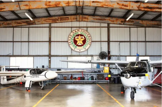
a synoptic overview of these aforementioned experiments. Three different aircraft have supported flight experiments and operations at TAMU-FRL including a Cessna O-2A Skymaster, Velocity XLRG-5, and a Stemme S10-V. The Skymaster and Stemme are shown hangared at the TAMU-FRL in Fig. 7. The Velocity and Stemme are no longer included in the TAMU-FRL fleet.

Fig. 7 Stemme S10-V (left) and Cessna O-2A Skymaster (right) hangared at TAMU-FRL

Cessna O-2A Skymaster

The test-bed aircraft utilized for this research is the Cessna O-2A Skymaster, which was manufactured in 1968 as a militarized version of the Cessna 337 Super Skymaster. The O-2A was flown in Vietnam for forward air control missions and was often equipped with Gatling-gun pods, bomblet dispensers and more frequently, rocket launchers. These different armaments were mounted utilizing any of the four hardpoints via pylons under

17

the aircraft’s wings. Another variant of the militarized Skymaster was the O-2B, which was used for psychological warfare in Vietnam (i.e. dropping leaflets and broadcasting messages via a fuselage mounted loud-speaker).

The O-2A was selected as the TAMU-FRL’s main research platform because of several advantageous aircraft features that aligned well with the needs of a specific boundary-layer stability and transition experiment, SWIFT. Those features include multiple engines, centerline thrust, retractable gear, four wing-mounted pylons for test articles, reinforced spars for cyclic loading, high wings coupled with observation windows on both the pilot and co-pilot sides, a third-row radio/instrumentation rack in the cabin, and jettisonable cabin door and pilot-side window in the event of an emergency evacuation (Carpenter 2009 [14]). Fig. 8 shows a detailed and dimensioned three-view schematic of the O-2A. Table 1 enumerates some of the major aircraft specifications.

18

19

Table 1 Cessna O-2A Specifications

Wingspan 38 ft Max Speed 192 KIAS

Length 29 ft Cruise Speed 120-130 KIAS

Height 9 ft Max Endurance 4.5 hrs + 0.5 reserve

Chord 5 ft Max GTOW 4300 lb

Service Ceiling 19,500 ft Engine (2x) IO-360 w/ 210 HP

2.2Overview and Comparison of SWIFT and SWIFTER

The present work will utilize a new model, shown mounted to the O-2A in Fig. 9 (middle right quadrant), called SWIFTER (Swept-Wing In-Flight Testing Excrescence Research) which was designed by Duncan (2014) [32]. The article mounted under the starboard wing of the O-2A in Fig. 9 (middle left quadrant) is a hotwire sting mount used previously for measuring freestream turbulence (Carpenter 2009 [14], Fanning 2012 [30]) and used currently as a ballast to partially offset the weight of SWIFTER. SWIFTER was designed specifically for investigating the influence of 2-D excrescences on laminar-turbulent transition in order to quantify a critical step height for manufacturing tolerances (Duncan et al. 2014 [32]). Like SWIFT, SWIFTER is a natural-laminar-flow airfoil that was designed to specifically study the isolated crossflow instability.

20

Fig. 9 SWIFTER and hotwire sting mount attached to the port and starboard wings of the Cessna O-2A Skymaster respectively (Photo Credit: Jarrod Wilkening)

SWIFT and SWIFTER, shown side-by-side in Fig. 10, share the same outer mold line (OML) or airfoil shape, 30° aft sweep, chord length of 1.372 m and span of 1.067 m. Retaining the same airfoil shape and design allows for direct comparison to previous experiments. This particular airfoil design was selected and continued for two major

21

reasons. First, SWIFT and SWIFTER were designed such that the crossflow instability is isolated by using the instability suppression techniques discussed in the Swept-Wing Boundary-Layer Stability and Transition section. Second, SWIFT and SWIFTER needed to be representative of a typical transport aircraft in both LE sweep (30°) and transport aircraft unit Reynolds number (Re′ = 4.0-6.0 x 106/m).

Fig. 10 SWIFT (left) & SWIFTER (right) side-by-side

While the shape of SWIFT and SWIFTER are identical, they differ extensively in construction. The most notable differences include an in-flight-moveable, interchangeable leading edge (15% chord and forward), improved low-infrared-reflective paint, internal heating sheet, secondary mid-span strut (mitigates deformation under aerodynamic loads),

22

pressure-side access panels and a lower overall weight. SWIFTER also has the capability to be mounted in a wind tunnel (Duncan et al. 2014 [33]). The paint and internal heating sheet will be discussed in the Infrared Thermography section.

As mentioned earlier, SWIFTER was specifically designed for testing 2-D excrescence influence on transition; therefore, the first 15% of the model is able to move via an internal actuation system (Fig. 11) to create steps and gaps. This actuation system, comprised of six linear actuators, six linear rail guides, two alignment shafts, two displacement sensors and an electromagnet, allows for LE alignment and step/gap configurations at the 15% chord location to an uncertainty of ±25 µm in the step direction. The additional mid-span strut assists in achieving this low level of uncertainty by minimizing relative displacement between the moveable LE and the main body of the model, especially in the test area (mid-span). The moveable LE can travel 20 mm (normal to the LE) out from the model along the chord line and ±5 mm in the chord-plane-normal direction to produce a wide range of step and gap configurations. This research employs a zero step configuration throughout the experiment. An expanded polytetrafluoroethylene gasket tape, made by Gore, provides the interface to seal the LE to the main body so that there is no suction or blowing at 15%. Further details of the SWIFTER model detail, design, and construction can be found in Duncan (2014) [32].

23

Fig. 11 SWIFTER airfoil graphic (top) and LE actuation system (bottom) (modified figure from Duncan 2014 [32])

2.3Five-Hole Probe and Calibration

Both SWIFT and SWIFTER utilized a conical-tip five-hole probe (5HP), manufactured and calibrated by the Aeroprobe company to measure model and aircraft attitude. The 5HP, in junction with four Honeywell Sensotech FP2000 pressure transducers, is used to measure α, θAC, q, and ps. In addition to model and aircraft attitude, the 5HP, in junction

with a static-temperature probe from SpaceAge Control that is mounted on the port, inboard hardpoint of the O-2A, measures freestream unit Reynolds number and altitude. Fig. 12 shows the static ring (left), conical tip (middle), and pressure port schematic of the 5HP. Model angle of attack (α) is measured differentially between ports 2 and 3, pitch

24

angle of the aircraft (θAC) is measured differentially between ports 4 and 5, dynamic

pressure (q) is measured differentially between port 1 (total-pressure) and the static ring, and finally freestream static pressure is measured absolutely using only the static ring.

Fig. 12 Five-hole probe (5HP): freestream static ring (left), conical tip (middle), pressure port schematic (right)

Improvements to the 5HP Mount and Alignment

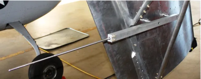
In order to reliably measure the attitude of the model (angle of attack and effective leading-edge sweep) the relative position of the 5HP to the model is crucial. Therefore, repeatable 5HP installation and position measurement is essential. The SWIFT 5HP (Fig. 13) was mounted to the non-test side of the model with a section of aluminum angle and a pair of bolts, washer shims and jam-nuts. This method of installation alone was often difficult in that the jam-nuts could slip from their original position during mounting; therefore, changing the position of the probe between removals and installations. After every installation the relative position (angle offset) would have to be measured. In order to quantify the offset of the 5HP to the chord line, the offset angle would be measured using a plumb bob to mark, on the hangar floor, the SWIFT chord line and a line following the shaft of the 5HP. These two lines would then be extended out to 35 ft (approximately

25

17.5 ft forward and aft of the model) so that the angle between the lines could be calculated. The process was to repeat this installation, alignment and measurement until the desired offset angle was achieved. This was a three person operation that was time intensive and largely susceptible to human measurement error.

Fig. 13 SWIFT five-hole probe mount

Conversely, the SWIFTER 5HP (Fig. 14) mounting process was much more simple and reliable. The 5HP was attached to the model using two bolts and two surface contour matching spacers that allowed for an accurate and repeatable installation every time. The process of removing and reinstalling the 5HP to SWIFTER was executed three times, and the relative position was measured after each installation using digital calipers and a digital level. The resulting average αoffset was -0.051° ± 0.008°, and the resulting θAC,offset was

2.02° ± 0.10°, both of which are within the measurement uncertainty (Duncan 2014 [32]). Instead of adjusting the alignment to obtain some specific offset, these numbers were simply accounted for when measuring model and aircraft attitude.

26

Fig. 14 SWIFTER five-hole probe mount

Improvements to the Pressure Transducer Box

In the SWIFT experiments, a significant source of uncertainty comes from the lack of temperature control for the Honeywell pressure transducers. The four transducers were calibrated at 22.8 °C, and therefore operate with a ±0.1% accuracy at that temperature. Furthermore, the transducers require a 1 hour warm-up time to ensure the quoted accuracies. If the temperature deviates from that calibration temperature, a temperature error of ±0.5% full scale must be added to the accuracy of the sensors. Additionally, that temperature error term is only valid if the transducers are operated in the 4 – 60 °C range. Outside of that range the transducers become unreliable. When cold-soaking the SWIFT model, a process that will be described in the Infrared Thermography section, the temperatures can easily drop to 0 °C.

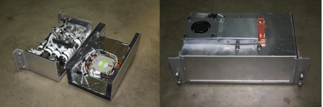
A solution to this problem, implemented in the SWIFTER model, was to construct (in house) a temperature controlled box to maintain the calibration temperature during flight operations. Fig. 15 shows the final temperature controlled system which involves a

27

thermoelectric cooler, 2 heat sinks & fans, insulation, a 100 Ohm resistive temperature detector (RTD) from Omega (for monitoring temperature) and a proportional-integral-derivative (PID) controller (for maintaining temperature). In addition to the temperature controlled pressure transducer box, the frequency response of the 5HP and pressure transducer system was improved by reducing the length of tubing between the 5HP tip and the transducers.

Fig. 15 Temperature controlled pressure transducer box

Improvements to the 5HP Calibration

The new SWIFTER 5HP was calibrated by Aeroprobe using a custom 996 point grid at Mach numbers of 0.2 and 0.3. This calibration was performed five times so that repeatability and hysteresis could be quantified. In addition to the calibration performed by Aeroprobe, an in-house calibration for α and θAC was performed using calibration

coefficients so that the dependence on measured dynamic pressure could be removed. It was discovered that significant non-linear effects were present as the orientation of the probe deviated from the 0° and 45° cross configurations. This non-linear behavior was not

28

accounted for in the SWIFT experiments which may have resulted in a measurement error of up to 3°. In order to most efficiently utilize the calibration coefficients, and obtain the best possible accuracy, curve fits with a quasi-constant coordinate were used. Additionally, large scatter in the residuals near zero were discovered in all calibration schemes. In order to avoid this scatter, the 5HP was canted 2° upwards in the θAC direction.

This offset was mentioned earlier when discussing probe alignment. The resulting α and

θAC RMSE and Pk-Pk for specific Mach numbers are enumerated in Table 2. The Mach

0.25 case has larger residuals because it was calculated by linear interpolation. This new probe and calibration scheme allows for extremely low total uncertainties in both α and

Re′ with values of ±0.10° and ±0.015 x 106/m respectively. A more in-depth description of the calibration and uncertainties can be found in (Duncan et al. (2013) [34] & Duncan (2014) [32]).

Table 2 RMSE and Pk-Pk values of the 5HP calibration (modified table from Duncan 2014 [32])

θAC Calibration α Calibration

Mach RMSE (°) Pk-Pk (°) RMSE (°) Pk-Pk (°)

0.20 0.12 0.85 0.03 0.35

0.25 0.18 1.12 0.07 1.21

0.30 0.13 0.70 0.06 0.69

2.4Infrared Thermography

Flow visualization is the primary method for studying laminar-turbulent transition in this research. In particular, infrared (IR) thermography is employed as the basis for determining the influence that DREs have on transition. IR thermography flow visualization provides real-time, high-fidelity measurements that are efficient and non-intrusive. The basic process of using IR thermography as a means of transition

29

detection is to force a temperature differential between the surface of the model and the ambient fluid. Turbulent flow will equalize the surface temperature to ambient faster than laminar flow due to the higher convection rate and surface shear stress. An IR camera is able to detect this difference in temperature, thereby delineating the location of laminar-turbulent transition. In this experiment, IR thermography is used to globally detect a transition front.

There are two methods of creating this surface-fluid temperature differential, which include wall cooling and wall heating. Additionally, both methods require a thin insulating layer on the surface that is capable of maintaining a strong temperature gradient. The SWIFT model employed the wall cooling technique, referred to as “cold soaking.” In this procedure, the model is cold soaked at an altitude in the range of 10,500 – 12,500 ft MSL for approximately 20 minutes. Upon uniformly cooling the SWIFT model, the O-2A rapidly descends through increasingly warmer air at lower altitudes in order to generate the temperature differential between the laminar and turbulent regions. During the dive in the wall cooling method, the turbulent region is heated faster than the laminar region due to the higher convection rate and shear stress. A main limitation to this process includes a larger fuel consumption to dive ratio. A typical SWIFT flight would only encompass two experimental dives due to the time and fuel required to climb to 10,500 ft MSL and loiter for 20 minutes before executing each experimental dive. Conversely, the SWIFTER model employed the wall heating technique in which the model is internally heated so as to bring the surface temperature to a few degrees above the ambient. Fig. 16 depicts the internal heating sheet, constructed from pre-sheathed heating wire and RTV (room temperature

30

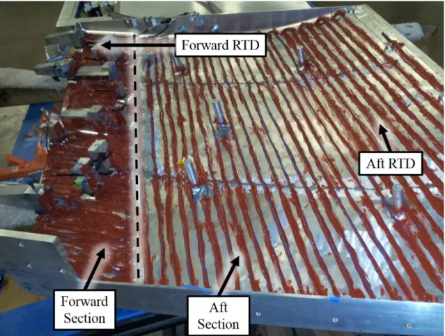
vulcanization) silicone. The heating sheet is divided into two sections (forward and aft) to accommodate for a discontinuous wall thickness. The temperature controller for the heating sheet is connected to three surface mounted RTDs. Two of the RTDs are for monitoring the heated surface, one for each heating sheet section, and the third is mounted to the unheated, non-test side as a reference temperature.

Fig. 16 SWIFTER heating sheet layout: Blue heating wire, Red RTV silicone, Insulation and reference RTD not pictured

31

This wall heating method precludes the need for a high altitude climb and cold soak, saving both time and fuel. In this procedure, the O-2A climbs to an altitude of 6,500 ft MSL, needs only a few minutes to confirm uniform heating before rapidly descending for the experimental dive. An average of 8 experimental dives can be completed in comparison to SWIFT’s 2. During the experimental dive, the turbulent region is cooled faster than the laminar region; again, this is due to the higher convection rate and shear stress of the turbulent flow. Fig. 17 shows a graphical representation of this process. In this case, the rapid descent is merely for achieving faster flow over the model and not necessarily aimed at utilizing the increasingly warmer air while descending in altitude. Because the model is actively heated, the surface is continuously a few degrees above the ambient fluid flow; however, it is important to note that the temperature lapse rate can overtake the heating sheet’s ability to maintain a higher surface temperature, and was experienced infrequently throughout the experimental campaign. The maximum power output of the heating sheet was approximately 500 W (Duncan 2014 [32]).

32

Fig. 17 Idealized graphic of wall heated model (not to scale) (top), Temperature distribution near transition (bottom) (Crawford et al. 2013 [35])

As mention earlier, successful IR thermography of boundary-layer transition requires a thin insulating layer on the surface that is capable of maintaining a strong temperature gradient. Additionally, the surface must be as minimally-reflective in the IR wavelength band as possible. The SWIFT model was coated in a flat black powder coat that held a strong gradient well; however, this powder coating was susceptible to reflections in the IR band. Features such as exhaust flare, diffraction of light around the fuselage, ground terrain and reflections of the test aircraft could be seen on the model. These reflections

33

could mask the transition process on the surface and contaminate the data. The SWIFTER model improved upon this drawback by utilizing Sherwin Williams F93 mil-spec aircraft paint in lusterless black. This coating provided the necessary insulation to achieve holding a strong temperature gradient, and also had low-reflectivity in the IR band. While some reflected features, mainly exhaust flare, could be observed, the contamination was miniscule. These features are actually removed utilizing the IR image post-processing code. SWIFTER’s paint thickness was approximately 300 µm in comparison to SWIFT’s 100 µm; the added thickness helps to sharpen any detail in the IR images.

IR Camera Comparison

At the start of the SWIFT experimental campaign, a FLIR SC3000 IR camera was used for transition detection. The SC3000 has a resolution of 320x240 pixels, operates in the 8-9 µm wavelength band, and can sample at a maximum frame rate of 60 Hz. Toward the end of the SWIFT campaign and for the entire SWIFTER campaign, a new updated IR camera was used, the FLIR SC8100. The SC8100 has a resolution of 1024x1024 pixels, operates in the 3-5 µm wavelength band, and can sample at a maximum frame rate of 132 Hz. The SC8100 has a temperature resolution lower than 25 mK. The SWIFT experiments utilized a 17 mm lens while the SWIFTER flight experiments utilized a 50 mm lens.

IR Image Processing

Throughout the entire SWIFT campaign and during the early stages of the SWIFTER DRE campaign, IR thermography was used as a qualitative transition detection tool. Transition location would be ascertained by human eye with an approximate uncertainty of x/c = ±0.05. These qualitative readings were very susceptible to human biasing error

34

and did not provide a consistent and accurate means of transition detection. However, this was initially seen to be sufficient for DRE experiments because substantial transition delay would be on the order of x/c = 0.1. Currently, quantifying the sensitivity of transition to DREs requires a more accurate and robust method of transition detection. Fig. 18 and Fig. 19 show an example of qualitative IR transition detection for the SWIFT and early SWIFTER campaigns respectively; these are raw IR images taken from the FLIR

ExaminIR software. It is clearly obvious that there is a large uncertainty in picking out the

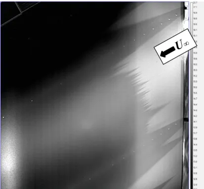
transition front. In Fig. 18, flow is from right to left, and the laminar, cooler region is denoted by the orange color, while the turbulent, warmer region is denoted by the yellow color. This is indicative of the wall cooling process where turbulent flow relatively heats the model surface. In Fig. 19, flow is diagonal from top-right to bottom-left, and the laminar, warmer region is denoted by the lighter shading, while the turbulent, cooler region is denoted by the darker shading. This is indicative of the wall heating process where turbulent flow relatively cools the model surface. In Fig. 19, more surface flow detail is observed when utilizing the SC8100 and the 50 mm lens.

35

Fig. 18 Raw IR image from SWIFT model with qualitative transition front detection at 50% chord. (modified figure from Carpenter (2009) [14])

36

Even with the improved IR camera and images, discerning the transition front was still susceptible to human biasing error. Brian Crawford (Crawford et al. 2014a [36]) developed a solution for this problem by creating an IR post-processing code that removes the human biasing error and inconsistency of qualifying transition location. Additionally, this code is able to reliably and repeatably pull out a quantitative transition-front location with an uncertainty on the order of x/c = ±0.001. This uncertainty does not include systematic errors found in α and Re′, but merely accounts for variations in front detection from frame to frame. It is essentially negligible compared to the systematic uncertainty. Total uncertainty for transition-location detection is ±0.025 x/c on average. Fig. 20 compares a raw (left) and processed (right) IR image, while quantifying a transition front location at x/c = 0.487 ± 0.001. Again, this uncertainty value does not account for systematic uncertainty. The blue dashed lines in Fig. 20 encompass the test area of the model. Additionally, Fig. 21 provides further perspective on the raw IR image orientation by overlaying it onto an image of the SWIFTER model in flight.

37

Fig. 20 Comparison of raw (left) and processed (right) IR images

38

The post-processing code involves four major steps: image filtering, fiducial/model tracking, image transformation, and transition detection. In order to remove any spatially slow-varying features, such as exhaust flare, sunlight on the model or internal structure illuminated by heating, the IR image is spatially high-passed. The image is then histogram normalized, so that contrast around temperatures with steep gradients are enhanced. This brings out a more defined transition front (aids in transition detection) and also makes the crossflow streaking clearly visible. Model tracking is accomplished by using three 50.8 mm square, Mylar tape fiducials, seen in Fig. 20. The highly IR-reflective Mylar tape provides a strong temperature gradient between the surface and itself by reflecting the cooler ambient temperature allowing for easy detection. Because the fiducials are placed at known locations on the model surface, the model orientation and position can now be characterized in 3-D space relative to the camera. Once model orientation and position are known, the raw IR image can then be transformed such that the chordwise direction is horizontal and the spanwise direction is vertical, with flow now from left to right (Fig. 20 (right)). This transformation step essentially “un-wraps” the surface of the model by accounting for viewing perspective, lens effects and model curvature. Finally, the transition front is located by calculating the gradient vector at every pixel in the filtered, tracked and transformed image. The resulting vector field is then projected onto the characteristic direction along which turbulent wedges propagate. The magnitude of these projections determines the likelihood of each point being a location of transition: larger projections are most likely transition while smaller projections are least likely transition. This continues until the code converges on an overall transition front.

39

Once the front is detected, 20 consecutive processed images, at the same experimental condition, are averaged together to obtain a single quantifiable transition front location. This is done by producing a probability density function (PDF), derived from a cumulative distribution function (CDF) of the front, for each of the 20 transition front locations. The abscissa (x/c location) of the PDF’s maxima corresponds to the strongest transition front. Graphically, it can be seen as the x-location of the largest peak in the PDF on the right side of Fig. 20. There are 20 colored lines representing each of the 20 analyzed images that are centered around 1 second of being “on condition.” Being “on condition” refers to holding a target α and Re′ within tolerances for 3 seconds during the experiment. Finally, the black curve is an accumulation of the 20 individual PDFs, thereby quantifying the most dominant transition location. A key feature to using PDFs is that they are unaffected by anomalies such as bug-strikes that would cast a single turbulent wedge. That turbulent wedge will receive a smaller PDF peak and not affect the more dominant larger peaks of the front location. Further detail on the IR post-processing code can be found in Crawford

et al. (2014a) [36].

2.5Traversing Laser Profilometer

Characterizing surface roughness is of key importance when conduction laminar-turbulent boundary-layer transition experiments. The surface roughness directly affects the receptivity process by providing a nucleation site for the initial disturbances. A Mitutoyo SJ-400 Surface Roughness Tester was used for characterizing all SWIFT LE configurations and for the polished LE of SWIFTER. This device is a contact stylus profilometer with maximum travel of 25.4 mm and a resolution 0.00125 µm when utilizing

40

the 80 µm vertical range setting. While this device can locally characterize surface roughness by means of the root-mean-square (RMS) and peak-to-peak (Pk-Pk), it is incapable of measuring frequency content in the wavelength band that strongly influences the crossflow instability (1-50 mm). To adequately resolve the power of a 50 mm wavelength on a surface, the travel of the profilometer must be able to acquire several times that length in a single pass. This need for surface roughness frequency analysis was met by the design and fabrication of a large-span, non-contact surface profilometer by Brian Crawford (Crawford et al. 2014b [37]). The traversing laser profilometer (TLP), shown in Fig. 22, utilizes a Keyence LK-H022 laser displacement sensor, has a chordwise-axis travel of 949 mm, a LE-normal-axis travel of 120 mm, surface-normal resolution of 0.02 µm, laser spot size of 25 µm, and is capable of sampling at 10 kHz. The TLP was used to characterize the surface roughness of the painted SWIFTER LE and to re-measure a previous SWIFT painted LE. Those roughness results will be discussed in the Surface Roughness section. The reason the TLP was not used to characterize the polished LE surface roughness was due to the noise generated by the laser reflecting off of the highly-polished surface. The noise floor was greater than the desired resolution to characterize the frequency content.

41

Fig. 22 Traversing Laser Profilometer with labeled components (modified figure from Crawford et al. 2014b [37])