MPRA
Munich Personal RePEc Archive
Estimating Fiscal Adjustments at the
Local Level in Colombia
Richard Jaimes
9 December 2016
Online at
https://mpra.ub.uni-muenchen.de/75507/
Estimating Fiscal Adjustments at the Local Level in
Colombia
∗
Richard Jaimes
†This draft: December 08, 2016
Abstract
The aim of this paper is to analyze how local governments in Colombia adjust their fiscal positions in response to budget imbalances. Using a panel data set of more than 450 municipalities and 26 departments over the period 1993 to 2013, I estimate a vector error-correction model in order to identify the level of discretion in policymaking at the local level in terms of fiscal reaction functions. I find that the local governments in Colombia commit to satisfy an intertemporal budget constraint. However, I also find that there are remarkable differences in the dy-namic adjustment governments follow in order to restore their fiscal position. For instance, departmental governments face greater fiscal constraints in compari-son with the municipal governments since these intermediate governments are financed largely by excise taxes and grants tend to respond in a lower extent to their budgetary innovations. Likewise, decomposing the municipal sample, I show that intergovernmental grants is a key variable for the majority of municipalities and that own-source revenues do not play an important role in fiscal adjustment patterns with the exception of large cities.
JEL classification: H70, H72, H77
Keywords: Fiscal adjustment; local fiscal policy; fiscal decentralization.
∗I would like to thank Hern´an Seoane for his valuable comments and guidance. I am also very
grateful to Shun-ichiro Bessho for sharing his code.
1
Introduction
There are large differences in budget deficits and public debt levels across local gov-ernments and over time in Colombia (Figures 1 and 2). In spite of this, little is known about the dynamic adjustment that governments follow in order to restore their fis-cal position. Understanding this process is crucial since during the last three decades, Colombia has embarked on a decentralization program which purpose has been to trans-fer responsabilities from higher levels of government to lower ones in order to improve the efficiency in service delivery (Manor, 1999; De Mello, 2000; Rodden, 2004).1
Never-theless, this process is still a work in progress (Bird, 2012). For instance, some authors claim that there is a weak sub-national own-revenue system, a problematic transfer system and important concerns about how to control sub-national spending in order to avoid overborrowing and overspending, so it is relevant to understand the economic and political constraints that sub-national units face when they react to changes in their budgets and the decisions they make (Mart´ınez, 2016; Faguet and S´anchez, 2014; Bird, 2012; Cort´es, 2010; S´anchez, 2006).
The Colombian case is interesting in itself since it is one of the most decentralized public systems in Latin America2. However, despite that the fiscal autonomy to raise own-source revenue and less transfer dependency are associated with higher levels of efficiency in delivering government services (Mart´ınez, 2016; Bird, 2012), the Colombian fiscal scheme relies on large portions of grants going to local budgets. Although to estimate the effect of grants or own-source revenues in delivery services is an important task, the purpose of this paper, instead, is to assess how local governments in Colombia adjust their fiscal positions in response to budget imbalances and determine which elements of the budget local governments alter given that those decisions could have relevant impacts in the provision of local public goods and, therefore, to affect the path of local economic growth (Alesina and Ardagna, 2013).3
In view of these challenges, I analyze how local governments in Colombia restore their fiscal solvency over time when they face unexpected changes in their fiscal deficits and public debt levels. Using a panel data set of approximately 500 municipalities and 26 departments over the period 1993 to 2013, I estimate a vector error-correction model in order to identify the level of discretion in policymaking at the local level in terms of fiscal reaction functions, assuming that the governments commit to satisfy an intertemporal budget constraint. In light of this, this research is aimed at furthering
1See Channa and Faguet (2012) for a comprehensive and recent survey of related empirical work
and its shortcomings given that the empirical evidence about the impact of more decentralized public systems on economic outcomes such as infant mortality rates, student test scores and school enrollment rates has pointed out mixed and inconclusive results (Blume and Voigt, 2011).
2For instance, the share of local expenditures in total public expenditures amounted from 18.5%
in 1995 to 36,8% in 2012 and transfers as percentage of national government expenditures rose from 46,7% in 1995 to 62,9% in 2012.
3For example, using data for OECD countries, Alesina and Ardagna (2010) show that in a process
of fiscal adjustment, spending cuts are associated with higher reductions in deficits and debt to GDP ratios which have positive effects on economic growth, in comparison with tax increases.
our understanding of the patterns of fiscal adjustment in Colombia, in particular, the role of the intergovernmental transfers in this context. To this end, I consider five fis-cal variables such as government consumption, government investment, debt services, own-source revenues, and intergovernmental transfers to describe those dynamic inter-relationships.
My contribution to the literature in this research is three fold. First, I revisit the question about the dynamic interrelationship between revenues and expenditures at the local level by using more disaggregated data on both the revenue and expenditure side. Second, I attempt to fill a gap in the literature by providing empirical evidence on the fiscal adjustment process at the sub-national level in a developing country. Third, given that the local governments show important differences in terms of their fiscal autonomy, types of expenditure and responsabilities (Bird, 2012), I compare the degree of fiscal adjustment in Colombia bearing in mind the type of government, the levels of population, the local GDP per capita and some fiscal decentralization indicators.
My results consistently show that intergovenrmental transfers play an important role in helping subnational units to reduce their fiscal deficits over time but in a lower extent for departments. Likewise, my estimations also highlight that there are perverse incentives in the Colombian fiscal scheme since local governments can induce more grants by increasing their spending regardless the category I define, that is, government consumption, government investment or debt service payments. Moreover, it is worth noting that own-source revenues respond more slowly to changes in other budgetary variables with the exception of large cities, which suggest that they could be in a better position to insurance themselves against common and idiosyncratic shocks.
The organization of the paper is as follows. In the next section, I present a brief literature review. In section 3, I describe a basic framework for understanding the intertemporal budget constraint at the local level. In the section 4, I present the data sets and point out their main characteristics. In Section 5, the empirical strategy is provided. Section 6 describes the specification tests used to estimate the model. In section 7, I point to the main results and perfom robustness checks. Section 8 concludes.
2
Related literature
This paper contributes to the literature that studies the dynamics of fiscal adjustment at the local level4. For instance, Buettner and Wildasin (2002, 2006) analyze these dynamic interrelationships using U.S. state local data that covers the period 1972 to 1997. They estimate a vector-error correction model distinguishing own-source revenue, grants, expenditures and debt service to point out which elements of the budget local government adjust in response to fiscal imbalances. They find that US states change in a greater extent their government expenditures in response to budget imbalances but they also present evidence that grants are highly sensitive to local fiscal deficits. In the same line, Buettner (2009) studies the German case during the period
2000 considering the role of fiscal equalization, through intergovernmental grants, on the local fiscal balances. He points out that intergovernmental transfers contribute to restore the fiscal position in German municipalities in a higher proportion than in US municipalities (two or three times greater). However, he also indicate that despite of fiscal equalization transfers, government spending is not less volatile in comparison with the results for US states.
Likewise, Sol´e-Oll´e and Sorribas-Navarro (2012) using the same methodology that Buettner et al (2006), describe the fiscal adjustment patterns in 258 municipalities in Catalonia, a Spanish region, during the period 1988 to 2006 and compare their results with those obtained for U.S. and Germany in order to take into account institutional arrangement differences. They find out that local governments have incentives to in-crease their expenditures due to expected bailouts from the central government and since the majority of sub-national units have a limited fiscal autonomy, the own-source revenue has a lower adjustment capacity in that environment.
In a recent work, Bessho and Ogawa (2015) analyze the Japanese case adopting the same vector-error correction model to estimate local fiscal adjustments. Using a sample of 3210 municipalities for the period 1977-2010 and separating the expenditure side into investment and current spending, they show that the government investment plays an important role in the adjustment process and that possibly there is presence of flypaper effects. Finally, other two related works to the analysis of the response to budget shocks, which follow the Buettner’s et al (2002, 2006) approach, Navon (2006) and Rattso (2004) describe the dynamics of the fiscal adjustment for the cases of Israel and Norway, respectively.
My main departure is that I measure fiscal adjustments to budget shocks at the local level in a developing country and divide the expenditure side into current expenditure, investment and debt service as in Bessho et al. (2015) and the revenue side into own-source revenue and intergovernmental transfers, which is an important element in the Colombian local budgets. Notice that Gemmel, Kneller and Sanz (2013) support the hypothesis that if local governments acquire more administrative powers or autonomy to mange their budgets, specially on the side of their revenues, then it will generate higher levels of investment and enhance economic growth. However, as Sanch´ez (2006) and Mart´ınez (2016) point out, intergovernmental transfers can have a negative effect on the local government behaviour in terms of limited incentives to increase their own-source revenues to finance local productive spending. So, it is particularly interesting to understand the impact of grants on other variables that compose the local budgets in the Colombian sub-national scheme.
3
Framework
Consider a small open economy. Following Bohn (2007), the standard budget constraint at datet for a particular local government i= 1, . . . , N can be written as follows:
Bi,t+1+Yi,t =Gi,t+ (1 +rt)Bi,t (1)
whereBi,t is the level of debt, Yit is total revenues,Gi,t is the non-interest spending,
and r > 0 is the exogenoues interest rate. Thus, I can define the with-interest deficit
Di,t as:
Di,t ≡Bi,t+1−Bi,t =Gi,t+rBi,t−Yi,t (2)
In this setting, Yi.t and Gi,t are given by:
Yi,t =Ri,t+Ti,t (3)
Gi,t =GCi,t+GIi,t (4)
whereRi,t is own-source revenues (taxation), Ti,t intergovernmental transfers, GCi,t
government consumption andGIi,t government investment. Hence, if I denote the debt
services rBi,t as DSi,t, then equation (2) can be rewritten as:
Di,t =GCi,t+GIi,t+DSi,t−Ri,t −Ti,t (5)
Likewise,B0 is exogenous and the transversality condition limt→∞ (1+Bt+1r)t = 0 holds,
as it is assumed in the literature, since all debts must be repaid. Notice that in this framework, given a initial level of debtBi,t, that in principle Ti,t is exogenous because
it is determined by central government rules and the international commodity prices, the local government chooses a spending levelGi,t, a level of debt for the next period
Bi,t+1 and how much to tax Ri,t in order to satisfy its intertemporal budget constraint.
4
Data Description
I observe annual budgetary information over the period 1993 to 2013 for 497 munic-ipalities and 26 departments in Colombia. The idea behind the use of two different samples is, by assessing the intertemporal linkages between local government expen-ditures and revenues, to compare results from departments and municipalities taking into account the differences among their institutional arrangements in terms of fiscal autonomy, types of expenditure, and responsabilities. I aggregate the budgetary data into five variables as stated above, that is: Government consumption, government in-vestment, debt services, grants and own-source revenues. The fiscal deficit is calculated as noted in equation (5).
I restrict the sample to local governments for which there is available data for 21 years. Since I am interested in studying whether local governments commit to satisfy an intertemporal budget constraint, the longer the sample period the better (Bohn, 1991). Notice also that I drop from the dataset municipalities and departments with inconsistent budgetary reports, that is, governments that report negative values for
government investment, government consumption, grants and/or own-source revenues. It is important to point out that despite of these changes, the dataset remains to be a representative sample of all local governments in Colombia. For instance, I keep a set of municipalities that amount in average 77% of total local government consumption, 72% of total investment, and 82,4% of total debt services. Likewise, 86% of total own-source revenues and 74% of total local GDP. For departments, the set amounts in average 90% of total own-source revenues, 82% of total population, 94% of total debt service payments and 87% of total departmental investment.
I decompose the revenue side in two items, the first one is own-source revenues which includes direct taxes, indirect taxes, user charges among others. The second one is in-tergovernmental grants which involves current and capital grants. Likewise, I divide government spending in three items, that is, government consumption, government investment and debt services. I compute government consumption as the difference between total spending and investment and debt services. The reason to follow that procedure is twofold. On the one hand, to evaluate the role of intergovernmental trans-fers in the fiscal adjustment path. On the other hand, to assess the trade-off that local governments face when they have to allocate their resources in terms of current expenditure and productive spending.
The source is the National Planning Department, with the exception of the price index and the population levels, which are obtained from the The National Adminis-trative Department of Statistics. All the variables are transformed in per capita basis and deflated to 2008 prices. Thus, values are expressed in hundreds of millons of 2008 Colombian Pesos (COP). I report the summary statistics for municipalities and depart-ments in Table 1 and Table 2, respectively. I present the mean, standard deviation, minimum and maximum values for each variable. Notice that in both samples, govern-ment investgovern-ment and intergoverngovern-mental transfers are the most volatile variables whereas debt service seems to be the most stable component in the local government budgets. This fact is related to the constraints that governments face, under the Colombian legal and administrative scheme, to borrow money for financing their expenditures.
Likewise, Figure 3 and Figure 4 show the paths of real fiscal variables in per capita terms for municipalities and departments, respectively. A salient feature in both fig-ures, to a certain extent, is the similar movement between government investment and grants over time. It is also worth noting that own-source revenues and government consumption follow the same pattern. This behaviour would imply that investment at the local level in Colombia depend highly on intergovernmental transfers and royalties which as suggested by Mart´ınez (2016) could have negative effects on the provision of local public goods e.g., corruption and poor governance. And that own-source revenues are used in a high proportion to pay wages and salaries and to purchase goods and services.
5
Empirical Strategy
To measure the fiscal adjustments to budget imbalances at the local level in Colombia for the period 1993-2013, I proceed to implement the Buettner’s et al (2002, 2006) approach. Since fiscal deficit inclusive of debt services turns out to be stationary, in line with Bohn(1991), government spending (consumption, investment, debt service) and government revenues (grants and own-source revenues) are cointegrated.5
Thus, I consider a vector error-correction representation of the fiscal deficit6, as defined in the previous section, in the following way:
∆Xit=θDi,t−1+
p
X
j=1
Ωj∆Xi,t−j +uit, i= 1, . . . , N, t= 1, . . . , T
where Xit = (GCit, GIit, DSit, Rit, Tit)0 and ψ = (1,1,1,−1,−1) forms the known
cointegrating vector. Thus, Dit = ψ0Xit. The idea behind this methodology is to
estimate the dynamic interrelationships between the variables that compose the local budget constraint assuming that the with-interest deficit is stationary in the long run. In this sense, θ and Ωj are the parameter matrices to be estimated. Hence, I proceed
with equation-by-equation OLS estimations without fixed effects and run robustness exercises in order to check the power of my results. Thus, I estimate the following system of equations: ∆GCit=θ1Di,t−1+a10+ p X j=1 a11,j∆GCi,t−j+ p X j=1 a12,j∆GIi,t−j + p X j=1 a13,j∆DSi,t−j+ p X j=1 a14,j∆Ti,t−j + p X j=1 a15,j∆Ri,t−j+u1it ∆GIit =θ2Di,t−1+a20+ p X j=1 a21,j∆GCi,t−j+ p X j=1 a22,j∆GIi,t−j + p X j=1 a23,j∆DSi,t−j+ p X j=1 a24,j∆Ti,t−j+ p X j=1 a25,j∆Ri,t−j+u2it
5There is a linear combination of budgetary elements that makes the fiscal deficit stationary, that
is, expenditures and revenues move together over time (L¨utkepohl, 2005).
6Notice that I need to check that the assumptions of the model are satisfied. That is, the deficit is
a I(0) process, and that five variables (GCit, GIit, DSit, Rit, Tit) are I(1) processes. Bearing in mind
that, I estimate the panel unit root test developed by Im, Pesaran and Shin (2003), which is widely used in the literature (see Table 3 and Table 6).
∆DSit =θ3Di,t−1+a30+ p X j=1 a31,j∆GCi,t−j+ p X j=1 a32,j∆GIi,t−j + p X j=1 a33,j∆DSi,t−j+ p X j=1 a34,j∆Ti,t−j+ p X j=1 a35,j∆Ri,t−j+u3it ∆Tit=θ4Di,t−1+a40+ p X j=1 a41,j∆GCi,t−j+ p X j=1 a42,j∆GIi,t−j + p X j=1 a43,j∆DSi,t−j + p X j=1 a44,j∆Ti,t−j+ p X j=1 a45,j∆Ri,t−j +u4it ∆Rit=θ5Di,t−1+a50+ p X j=1 a51,j∆GCi,t−j+ p X j=1 a52,j∆GIi,t−j + p X j=1 a53,j∆DSi,t−j+ p X j=1 a54,j∆Ti,t−j + p X j=1 a55,j∆Ri,t−j+u5it
To interpret the results, I calculate impulse-response functions (fiscal reaction func-tions) in present-value terms following Bohn (1991) and Buettner et al. (2002, 2006). By doing that, I can estimate how future local fiscal policy responds to unexpected changes in current fiscal variables. Firstly, I plot impulse-response functions for each variable and type of government (see Figures 5-14) assuming that there are not con-temporaneous effects between the variables as proposed by Buettner et al. (2006). Secondly, following the procedure of Bessho et al. (2015) I summarize the results us-ing present value responses to temporal and permanent innovations usus-ing a Cholesky decomposition identification scheme using the variance-covariance matrix.
Note that this identification strategy imposes additional constraints (zero short-run restrictions on contemporaneous coefficients) since I need to assume the order of the variables to get back to the structural representation and to attain identification of the system (Hamilton, 1994). Thus, I begin ordering government spending variables first (government consumption, government investment, debt service) and then rev-enue variables (intergovernmental grants and own-source revrev-enues). This specific order implies that revenues respond contemporaneously to government spending shocks but expenditure variables do not respond to innovation in revenue variables within the pe-riod. Although this particular approach do not follow a theoretical counterpart, the results are robust to changing the Cholesky ordering, that is, the estimated impacts are qualitatively similar and the quantitative differences are small. It is also worth noting that the point estimates do not differ so much from the ones estimated assuming no contemporaneoues responses.7
6
Specification tests
As stated above, to estimate a vector error-correction model I need to verify that its assumptions are satisfied. Therefore, I proceed to check that the deficit is a I(0) process, and that five variables (GCit, GIit, DSit, Rit, Tit) are I(1) processes. In order
to do that, I use the Im, Pesaran and Shin’s (2003) test which allows me to control for heterogeneity and serially correlated errors. Likewise, to determine the number of lags8
to be included in the OLS estimations and to assess the existence of local fixed effects9, I estimate likelihood ratio tests on cross-equation restrictions following the procedure proposed by Hamilton (1994).
6.1
Panel unit-root tests
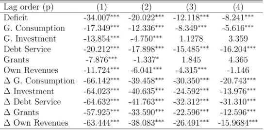
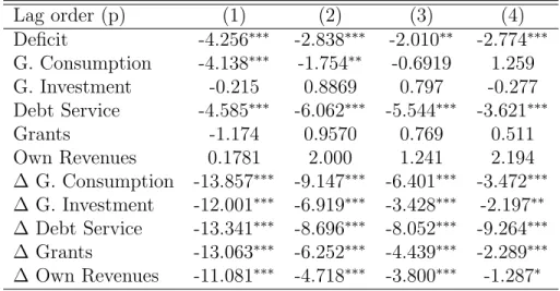
In this subsection, I present the results of panel unit-root tests for each fiscal variable in order to determine their stationarity. Table 3 and 6 reports the unit-root statistics for municipalities and departments, respectively. The tests for variables in levels include a time trend with the exception of fiscal deficit. I also use different lag orders to control for serially correlated errors. These calculations suggest that the fiscal deficit is stationary and that the first differences of the other budgetary components are also stationay in both samples regardless the lag order which support the use of the VECM model. I also display the results for the variables in levels. Notice that I cannot reject the null hypothesis that all the panels contain unit roots for both goverment investment and grants in levels for municipalities. And for departments, I reject stationarity in leves for government consumption, government investment, grants and own-source revenues.
6.2
Lag selection and local-fixed effects
In order to determine the optimal lag order I begin by using four lags for each variable as suggested by the previous literature, then I test for a possible reduction in this number. It is also worth noting that I do not include local fixed effects10 since I introduce variables in first differences and, to certain extent, I could assume that all local governments should converge to the same deficit level e.g. zero (Buettner, 2009; Sol´e-Oll´e et al., 2012, and Bessho et al, 2015). I check these assumptions using likelihood
8According to previous literature, the majority of studies have employed a lag length of four years. 9I do not include time-specific effects since the intertemporal budget constraint should respond to all
innovations and not only to idiosyncratic shocks (Buettner et al, 2006; Buettner, 2009). Nevertheless, I estimate the model using time effects and the results are quite similar. Estimations are available upon request.
10Note that the literature recommend to use instrumental variables techniques in dynamic panel
data models when regressors include lagged dependent variables in order to reduce the OLS estimate bias in short panels (Buettner, 2009). However, since my sample only contains 21 years for each unit the Nickell (1981) bias should not be large and as suggested by Buettner et al. (2006) and Buettner (2009) I could neglect this bias when I proceed to test for local-fixed effects.
ratio tests on cross-equation restrictions, using the variance-covariance matrix of the residuals for the set of five equations of my model.
Tables 4 and 7 report the likelihood ratio statistics for each sample. For instance, for the specification of lag order in the first column, the null hypothesis is that the dynamics of the model are captured by three lags, and the alternative hypothesis suggests to use four lags. The reduction of lags is always rejected in both models, so in the below estimations, I use a specification with four lags. Likewise, to assess for the necessity of including local-fixed effects11, I calculate likelihood ratio tests with different lag order in which the null hypothesis is that the model does not require the use of local-fixed effects. I cannot reject this hypothesis in any specification, so for the next exercises, I proceed with equation-by-equation OLS estimations without fixed effects since joint estimation does not provide gains in efficiency given that I use the same set of variables in each equation (Batalgi, 1995; Sol´e-Oll´e et al., 2012).
7
Main results
In the next subsections, I show the main results for both samples by identifying the type of innovation e.g., temporal or permanent, and the reponse for each variable. Thus, I present municipal and departmental reponses to a positive innovations in budgetary elements over the period of ten years (see Figures 5-14). As expected, since the variables are not mean reverting, the impact of innovations do not die out over time, which implies that innovations in this system have permanent effects on the elements composing the government budget constraint. Moreover, these results show that adjustments take place in the first six-seven periods indicating that local governments require long periods of time to restore their fiscal positions. For the estimations of the present value responses, I assume, as the previous literature, a discount rate of 3%, and interpret the results according to the procedure of Buettner et al., (2006) and Bessho et al., (2015) in order to compare them with related studies.12
7.1
Results in Colombian municipalities
Table 10 displays the estimates for the error correction term in the sample of Colombian municipalities. The vector of coefficientsθ confirms the error-correction representation
11I include individual local-fixed effects in all equations for both samples. Notice that for
munic-ipalities using Hausman tests I can reject the null hypothesis that the random effects model should be used (see Table 5) since the difference in coefficients is not systematic. For departments, instead, Hausman tests suggest to use random effect models (see Table 8) , but once I calculate Breusch-Pagan Lagrange Multiplier test to evaluate the hypothesis of no significant difference across units, the results indicate that OLS estimates should be preferred (see Table 9). Since this kind of tests could no have so much sense using variables in first differences, I use likelihood-ratio test as in previous literature about fiscal adjustments (Buettner et al., 2006; Buettner, 2009; Sol´e-Oll´e et al., 2012; and Bessho et al., 2015).
of the fiscal deficit and supports the assumption that the intertemporal budget con-straint holds in the long run. Notice that a higher deficit has a negative effect in both types of local government spending e.g., consumption and investment. Likewise, it has a positive effect in both grants and own-source revenues. Debt services respond pos-itively which indicates that a higher deficit results in a rise in debt and, therefore, a higher level of debt services.
Table 11 reports the implied present value responses of each fiscal variable to inno-vations in both itself and other variables. The columns show how fiscal variables adjust after a specific innovation in the system and the rows present how a particular variable reacts to unit changes in other variables. For instance, a 1 COP positive innovation in goverment consumption in one period is followed by a reduction in future gover-ment consumption of 47 cents and in govergover-ment investgover-ment of 8.2 cents. Grants and own-source revenues react positively to this innovation with an increment of 30.6 cents and 11.3 cents, respectively. Given that this rise in government consumption could be financed through debt, there is positive effect on debt services of 16 cents. All of these responses are statistically significant and have the expected sign.
Furthermore, a 1 COP positive unexpected change in government investment leads to a decrease in future government investment of 75 cents, which implies that the level of investment is 25 cents above the level before the innovation takes place. Notice that in this case, government consumption decreases in 1 cent and debt services increase in 6 cents. It is also worth noting that grants and own-source revenues reacts in a lower extent to a government investment rise (17.8 cents and 3.5 cents, respectively) than to a government consumption increase. All of these responses are statistically significant and have the expected sign.
A positive unit innovation in grants is followed by a reduction in future grants of 69 cents and 2.5 cents in own-source revenues. The latter impact supports the idea that municipalities whose receive more grants tend to decrease their fiscal effort (Mart´ınez, 2016; Faguet et al., 2014), however, this effect seems minimal. Notice that these results also confirm a possible fly-paper effect in Colombian municipalities given that grants have a positive and significant effect in future spending, particularly in investment, with a total increment of 25 cents. These point estimates are in line with the ones reported for US states where a rise in grants of US$ 1 generates an increment in expenditures of 33 cents (Buettner et al., 2006) and for Spanish municipalities where there is a rise in local spending of 28 cents due to an increment in grants (Sol´e-Oll´e et al., 2012). It is important to mention that grants have significant and positive responses to innovations in local public spending which suggest that there is a soft-budget constraint problem given that municipalities may follow an opportunistic behaviour (Bessho et al, 2015).
Moreover, a positive innovation in own-source revenues of 1 COP leads to a decrease in grants of 9.1 cents and in future own-sources of 55 cents. The impact on debt services has the expected sign but it is not significant. Government investment reacts positively with a future increment of 29.3 cents and government consumption with 3.6 cents. Notice that these impacts are higher in comparison with the responses due to innovations in grants. This fact can be explained bearing in mind that when government
revenues come from local taxation and not from a external source e.i., grants, voters can force to local governments to increase productive spending (Mart´ınez, 2016).
As suggested by the previous studies, it is also instructive to calculate the responses to permanent innovations (Bessho et al. 2015; Sol´e-Oll´e et al, 2012; Buettner, 2009; Buettner et al., 2006). The bottom of the Table 8 reports those present value responses. Notice that a permanent positive unit innovation in both government consumption and investment is followed by an increment in grants of 58 cents and 71 cents, respectively, supporting again the existence of a soft-budget constraint problem. In addition, future own-source revenues increase by 21.2 cents and by 14.1 to a unit permanent innovation in government consumption and government investment, respectively. These impacts are similar to the ones computed for Spanish municipalities where the response of own-source revenues to a permanent innovation in total local spending attains 31 cents (Sol´e-Oll´e et al., 2012). However, these effects are lower if I compare them with the point estimates reported by Buettner et al., (2006) for the US states (57 cents), by Bessho et al., (2015) for the Japanese municipalities (51 cents), and by Buettner (2009) for the German municipalities (43 cents). This could imply that Colombian municipalities face limited fiscal autonomy in terms of capacity to increase their own-source revenues as Bird (2012) suggests.
It is also interesting assess the response of primary surplus to innovations in each fiscal variable in order to check whether the Colombian municipalities commit to sat-isfy an intertemporal budget constraint. Indeed, summing up the responses of fiscal variables that conform the primary surplus, it follows that the absolute value of the changes are close to unity in all cases, but not for debt services (see Table 12). Ac-cording to Buettner et al., (2006) and Buettner (2009), the latter result in which the fiscal balance is not achieved in response to innovations in debt services, could reflect temporal fluctuations in this fiscal variable. Notice that the present value response of debt services to a unit innovation in itself is -0.483 COP, which implies that 0.517 COP of this innovation is permanent. If I compare this value with the present value of the change in primary surplus (0.486) due to a unit innovation in debt services, then I can claim that this result is in line with the predictions derived from an intertemporal budget constraint approach (Bessho et al., 2015; Buettner, 2009).
7.2
Results in Colombian departments
Table 13 reports the estimates for the error correction term in the sample of Colombian departments. Notice that a higher deficit has a significant and negative effect in local government spending. Likewise, it has a signficant and positive effect in own-source revenues. Grants reacts positively to a higher deficit but the point estimate is not significant. Moreover, Debt services respond positively which indicates that a higher deficit results in a rise in debt and, therefore, a higher level of debt services, but its coefficient is not significant. Government consumption does not have the expected sign but its estimate is not statistically significant.These results could indicate that Colom-bian departments face greater fiscal constraints than the ColomColom-bian municipalities to
extract grants from the national government. Thus, given that reducing government investment entails welfare losses, Colombian departments have to rely on more in own-source revenues in response to higher deficits, even though their capacity to generate fiscal resources is limited, since these intermediate governments are financed largely by excise taxes and intergovernmental grants tend to respond in a lower extent to their budgetary innovations (Acosta and Bird, 2005).
Table 14 shows the implied present value responses of each fiscal variable to inno-vations in both itself and other variables for Colombian departments. As suggested above, given the structure of the departmental finances, these local governments tend to restore their fiscal position using government investment and own-source revenues in a lower extent. For instance, a positive unit innovation in government consumption is followed by a statistically significant reduction in government investment of 40 cents whereas in municipalities the impact attains only 8 cents. Likewise, a positive inno-vation in government investment of 1 COP leads to a decrease in future productive spending of 81 cents, so investment at the departmental level is highly volatile. The other responses are not statistically significant, though they have the expected signs.
Furthermore, there is also evidence of a fly-paper effect in Colombian departments since a positive unit innovation in grants is followed by a reduction in own-source revenues of 14 cents and an increment of 49 cents in government investment. It is worth noting that this impact is higher than for my sample of Colombian municipalities. Moreover, the response is greater when the innovation in grants is permanent giving as result an increment in future local investment of 86 cents and a reduction in future own-source revenues of 26 cents. If I compare the latter point estimate with previous studies in other countries, only Buettner et al., (2006) reports a similar reduction (27 cents) for the US states. But for municipalities in Germany, Japan, Colombia and Spain the response of own-source revenues to a permanent positive unit innovation in grants is -4 cents, -2 cents, -8 cents and -7 cents, respectively (Buettner, 2009; Sol´e-Oll´e et al., 2012; Bessho et al., 2015). This result can be explained by the fact that the few responsabilities of departmental governments, basically in national programs for providing health and education services, can be financed with national transfers, so indeed, there is no incentive to find out new sources of revenues (Bird, 2012; Acosta et al., 2005).
Using the same procedure as before, Table 15 assess the response of primary sur-plus to innovations in each fiscal variable in order to check whether the Colombian departments commit to satisfy an intertemporal budget constraint. Notice that the absolute value of the changes are close to unity in all cases, but not for debt services. As mentioned above, it is due to temporal fluctuations in that fiscal variable.
7.3
Additional results: Decomposing the municipal sample
In this subsection, I proceed to assess whether the above results about fiscal adjustment at the local level in Colombia change when I decompose the municipal sample bearing in mind the important differences in population levels, their local GDP per capita and
their degree of fiscal decentralization, which takes into account their fiscal autonomy and other administrative capacities. A common perception in the economic literature is that Colombian municipalities have profound disparities, different natural resource abundance, partial fiscal decentralization, high levels of public sector corruption, limited economic opportunities for people, distinct growth rates and almost no discretion on public spending (Mart´ınez, 2016; Bird, 2012). For instance, it is possible that larger or richer cities follow different patterns of fiscal adjustment since they could have access to more resources and receive more political support from the national goverment.
Table 16 shows the implied present value responses with respect to city size. I decompose the sample in quartiles using the long-run distribution of population as in Buettner et al., (2006). I only report the results for large cities (top quartile) and small cities (bottom quartile). From the comparison of the point estimates between subsam-ples, it follows that indeed large cities respond increasing their own-sources revenues in a greater extent than the small cities to a temporal positive unit innovation in both government consumption and government investment with a value of 20 cents and 10 cents, respectively. The difference is even bigger when the innovations in local spend-ing are permanent. Surprisspend-ingly, the impact on government spendspend-ing of unexpected changes in both own-source revenues and grants are quite similar regardless the size of the city. However, notice that the volatility of government expenditures, grants and own-source revenues in small cities is greater than in large cities. These results could imply that large cities are in better position to insurance themselves against common and idiosyncratic shocks.
Furthermore, using the local GDP per capita13 as an indicator variable of local development, Table 17 displays the present value responses for cities in the top and bottom quartiles for the average local GDP per capita distribution over the period 2000-2009. It is worth noting that for municipalities in the bottom quartile, grants from the national government respond to a greater extent than for municipalities in the top quartile to innovations in any variable of the system. This impact could be explained by the fact that grants in Colombia are distributed following constitutional rules which are based on social indicators e.g., education attainment, mortality rates, poverty level, so the majority of grants are relatively designate to poor municipalities in order to close profound prosperity gaps. In this line, note that the negative impact on own-source revenues of unexpected changes in grants is only statistically significant for municipalities in the bottom quartile, giving as result a reduction of 34 cents in response to a permanent unit innovation in intergovernmental transfers. It turns out that although transfers go to the more needed municipalities, it is also true that this fiscal scheme generates perverse incentives in those local governments.
In addition, I also exploit the variation in the average fiscal decentralization index-FDI- prepared by the National Planning Department over the period 2000-2013 to assess whether municipalities with better administrative capacities, higher fiscal effort, and
13The dataset is obtained from the Center for Economic Development Studies-CEDE (Universidad
lower dependence on grants, follow a different pattern in terms of fiscal adjustments. Table 18 reports, for instance, that a 1 COP positive innovation in grants is followed by a rise of 26 cents in government investment for municipalities in the top quartile for the average FDI distribution, whereas by 21 cents in the same fiscal variable for municipalities in the bottom quartile. Moreover, as expected, grants for municipalities in the bottom 25% react in a greater extent to innovations in local spending than for governments in the top quartile. However, the response of own-source revenues to innovations in both government consumption and government investment are quite similar for both subsamples.
8
Conclusions
In this paper, I analyze how local governments in Colombia react to innovations in the fiscal variables that compose their budgets. Using a vector error-correction model I identify the level of discretion in policymaking at the local level in terms of fiscal reaction functions. In particular, I find that local governments in Colombia during the last 20 years have followed corrective actions in order to satisfy an intertemporal budget constraint. However, I also find that departmental governments face greater fiscal constraints to restore their fiscal positions in comparison with the municipal gov-ernments. The nature of this difference has to do with the fact that departments have lower fiscal capacity to increase their own-source revenues, almost no discretion on public spending and that their responsabilities are highly financed by grants from the national government.
Furthermore, although the results for Colombian municipalities are in line with the effects that report some international studies in developed economics eg., Spain, United States, Japan or Germany, when I decompose the municipal sample taking into account important differences in population levels, local GDP per capita gaps and several degrees of fiscal decentralization, I find, for instance, that intergovernmental grants is a key variable for the majority of municipalities and that own-source revenues do not play an important role in fiscal adjustment patterns with the exception of large cities.
References
[1] Acosta, Olga L., & BIrd, Richard. 2005. The Dilemma of Decentralization in Colom-bia, in: Richard M. Bird, James M. Poterba, & Joel Slemrod (eds.), Fiscal Reform in Colombia: Problems and Prospects, Cambridge, MA: MIT Press, pp. 247-286 [2] Alesina, Alberto., & Ardagna, Silvia. 2013. The Design of Fiscal Adjustments. In:
Brown, Jeffrey R. (ed.). Tax Policy and the Economy, Vol. 27, University of Chicago Press, pp. 19-67.
[3] . 2010. Large Changes in Fiscal Policy: Taxes versus Spending. In: Brown, Jeffrey R. (ed.). Tax Policy and the Economy, Vol. 27, University of Chicago Press, pp. 35-68.
[4] Batalgi, Badi H. 1995. Econometric Analysis of Panel Data. Wiley, New York. [5] Bessho, Shun-ichiro & Ogawa, Hikaru. 2015. Fiscal adjustment in Japanese
munic-ipalities. Journal of Comparative Economics, Vol. 43, 4, pp. 1053-1068
[6] Bohn, Henning. 1991. Budget balance through revenue or spending adjustments? Some historical evidence for the United States. Journal of Monetary Economics, 27, pp. 333-359.
[7] . 2007. Are stationarity and cointegration restrictions really necessary for the intertemporal budget constraint?. Journal of Monetary Economics, 54, pp. 1837-1847.
[8] Bird, Richard. 2012. Fiscal decentralization in Colombia: A work (still) in progress. International Center for Public Policy. WP, 12-23.
[9] Blume, Lorenz y Voigt, Stefan. 2011. Federalism and decentralization – a critical survey of frequently used indicators. Constitutional Political Economy. Vol. 22, (3), pp. 238-264.
[10] Buettner, Thiess & Wildasin, David E. 2006. The dynamics of municipal fiscal adjustment. Journal of Public Economics, 90, pp. 1115-1132.
[11] . 2002. The dynamics of municipal fiscal adjustment. CESifo Working Paper Series 649, CESifo Group Munich.
[12] Buettner, Thiess. 2009. The contribution of equalization transfers to fiscal adjust-ment: Empirical results for German municipalities and a US-German comparison. Journal of Comparative Economics, 37, pp. 417-431
[13] Channa, Anila y Faguet, Jean-Paul. 2012. Decentralization of health and educa-tion in developing countries: a quality-adjusted review of the empirical literature. Economic organisation and public policy discussion papers. EOPP 38. STICERD, London, UK.
[14] Cort´es, Darwin. 2010. Do more decentralized local governments do better? An evaluation of the 2001 decentralization reform in Colombia. Documentos de Trabajo No. 007182. Universidad del Rosario. Facultad Econom´ıa.
[15] Faguet, Jean-Paul & S´anchez, Fabio. 2014. Decentralization and Access to social services in Colombia. Public Choice, Vol. 160, 1, pp. 227-249
[16] Gemmell, N., Kneller, R. and Sanz, Ismael. 2013. Fiscal Decentralization and Economic Growth: Spending versus Revenue Decentralization. Economic Inquiry, Vol. 51, 4, pp. 1915-1931.
[17] Hamilton, James. 1994. Time Series Analysis. Princeton University Press.
[18] Im, Kyung So., Pesaran M. Hashem & Shin, Yongcheol. 2003. Testing for unit roots in heterogeneous panels. Journal of Econometrics, Vol. 115, 1, pp. 53-74 [19] L¨utkepohl, Helmut. 2005. New Introduction to Multiple Time Series Analysis.
Springer-Verlag Berlin.
[20] Manor, James. 1999. The Political Economy of Democratic Decentralization. Di-rections in Development. The World Bank.
[21] Martin-Rodriguez, Maria & Ogawa, Hikaru. 2016. The Empirics of the Municipal Fiscal Adjustment. Journal of Economic Surveys, Vol.00, 0, pp.1-23
[22] Mart´ınez, Luis R. 2016. Sources of Revenue and Government Performance: Evi-dence from Colombia. Working Paper. LSE.
[23] Navon, Guy. 2006. Budgetary dynamics in the local authorities in Israel. Israel Economic Review, 2, pp. 19-52
[24] Nickell, Stephen. 1981. Biases in Dynamic Model with fixed effects. Econometrica, Vol. 49, 6, pp. 1417-1426
[25] Rattso, Jorn. 2004. Fiscal adjustment under centralized federalism: empirical eval-uation of the response to budgetary shocks. FinanzArchiv, 60, pp. 240-261
[26] Rodden, Jonathan. 2002. The Dilemma of Fiscal Federalism: Grants and Fiscal Perfomance around the World. American Journal of Political Science. Vol. 46, (3), pp. 670-687.
[27] S´anchez, Fabio. 2006. Descentralizaci´on y Progreso en el Acceso a los Servicios Sociales de Educaci´on, Salud y Agua y Alcantarillado. Documentos CEDE. No. 2006-15. Universidad de Los Andes.
[28] Sol´e-Oll´e, Albert & Sorribas-Navarro, Pilar. 2012. The dynamics adjustment of local government budgets: does Spain behave differently?. Applied Economics, 44, pp. 3203-3213.
Appendix A
I calculate the implied present value responses according to Buettner et al., (2006) and Bessho et al., (2015). The vector error-correction model is given by the following set of equations: ∆Xit =θDi,t−1+ p X j=1 Ωj∆Xi,t−j +uit
where Xit = (GCit, GIit, DSit, Rit, Tit)0 and ψ = (1,1,1,−1,−1) forms the known
cointegrating vector. Hence, Dit = ψ0Xit. Using the fact that I can write the fiscal
deficit asDi,t−1 =ψ∆Xi,t−1+Di,t−2, following Bohn (1991) and Buettner et al., (2006),
I set up a first-order VAR to computed impulse-response functions:
Zi,t =FZi,t−1+vi,t
such that F≡ Ω1+θψ0 Ω2+θψ0 Ω3+θψ0 Ω4+θψ0 θ I 0 0 0 0 0 I 0 0 0 0 0 I 0 ... 0 · · · 0 ψ0 1 , Zt≡ ∆Xt ∆Xt−1 ∆Xt−2 ∆Xt−3 Dt−4 , vt≡ ut 0 .. . 0
where Fis a (21×21) matrix, Iis a (5×5) identity matrix and 0 is a (5×5) zero matrix. Thus, the prediction of the k-period ahead value of Zi,t in response to a unit
innovation in period t is given by: ˆ
Zt+k=Fkvi
where vi identifies the i-th budget component in which the innovation takes place.
Using a row-selection vector hj, which identifies the j-th element of interest included
in the vector Zt+k, it is possible to compute the present value of the response of the
j-th budget element with respect to a unit innovation in the i-th component, in the following way:
ˆ
π(j, i) =X
k≥1
hjρkFkvi =hjρF[1−ρF]−1vi
where ρ= 1/(1 +r) is the discount factor and r is the given interest rate (fixed at 3%). The responses to permanent innovations are calculated as follows:
ˆ
π(j, i) 1−πˆ(j, i)
Figure 1: Municipal Heterogeneity across years in fiscal deficits, 1993-2013
Note: Per capita basis and deflated to 2008 prices. The black line with diamonds represents the fiscal deficits mean for each year. Source: National Planning
Department; author’s calculations.
Figure 2: Departmental Heterogeneity across years in fiscal deficits, 1993-2013
Note: Per capita basis and deflated to 2008 prices. The black line with diamonds represents the fiscal deficits mean for each year. Source: National Planning
Table 1: Descriptive statistics (1993-2013, 497 Municipalities)
Variable Mean Std. Dev. Min. Max.
G. Consumption 0.112 0.061 0 0.803 G. Investment 0.426 0.327 0 3.735 Debt Services 0.007 0.011 0 0.28 Grants 0.398 0.294 0.004 3.7 Own-Source Revenues 0.136 0.13 0.001 1.332 Deficits 0.011 0.127 -1.861 1.743 Population 53029.2 332718.4 664 7674366
Source: National Planning Department; author’s calculations.
Values expressed in hundreds of millons of 2008 Colombian Pesos (COP).
Figure 3: Trends of fiscal variables in Colombian Municipalities
Note: Per capita basis and deflated to 2008 prices. Source: National Planning Department; author’s calculations.
Table 2: Descriptive statistics (1993-2013, 26 Departments)
Variable Mean Std. Dev. Min. Max.
G. Consumption 0.116 0.130 0.010 1.441 G. Investment 0.498 0.502 0.001 3.417 Debt Services 0.010 0.021 0 0.218 Grants 0.431 0.433 0 2.351 Own-Source Revenues 0.192 0.203 0.021 1.912 Deficits 0 0.172 -1.023 0.949 Population 1096838 1268973 23869 6299990
Source: National Planning Department; author’s calculations.
Values expressed in hundreds of millons of 2008 Colombian Pesos (COP).
Figure 4: Trends of fiscal variables in Colombian Departments
Note: Per capita basis and deflated to 2008 prices. Source: National Planning Department; author’s calculations.
Table 3: Panel unit-root tests for municipalities Lag order (p) (1) (2) (3) (4) Deficit -34.007∗∗∗ -20.022∗∗∗ -12.118∗∗∗ -8.241∗∗∗ G. Consumption -17.349∗∗∗ -12.336∗∗∗ -8.349∗∗∗ -5.616∗∗∗ G. Investment -13.854∗∗∗ -4.750∗∗∗ 1.1278 3.359 Debt Service -20.212∗∗∗ -17.898∗∗∗ -15.485∗∗∗ -16.204∗∗∗ Grants -7.876∗∗∗ -1.337∗ 1.845 4.365 Own Revenues -11.724∗∗∗ -6.041∗∗∗ -4.315∗∗∗ -1.146 ∆ G. Consumption -66.142∗∗∗ -39.458∗∗∗ -30.350∗∗∗ -20.743∗∗∗ ∆ Investment -64.023∗∗∗ -40.635∗∗∗ -24.592∗∗∗ -13.976∗∗∗ ∆ Debt Service -64.632∗∗∗ -41.763∗∗∗ -32.312∗∗∗ -31.310∗∗∗ ∆ Grants -57.925∗∗∗ -33.590∗∗∗ -22.596∗∗∗ -12.596∗∗∗ ∆ Own Revenues -63.444∗∗∗ -38.083∗∗∗ -26.491∗∗∗ -15.9684∗∗∗
Note: Im, Pesaran, and Shin’s (2003) test. Wtbar statistic is reported.
The sample period is 1993-2013, the number of observations is 10437.
∗ p <0.10,∗∗ p <0.05,∗∗∗ p <0.01
Table 4: Specification tests in Colombian municipalities Lag order (p) 4→3 3→2
χ2(25) 1054.31 [0.000] 1285.64 [0.000]
Municipality-fixed effects? With lag length=4 With lag length=3
χ2(2480) 2134.21 [1.000] 1818.30 [1.000]
Likelihood-ratio statistics on cross-equation restrictions; [ ]: p-values
Table 5: Hausman tests for the basic model in municipalities Equation ∆GCi,t ∆GIi,t ∆DSi,t ∆Ti,t ∆Ri,t
χ2(21) 165.21 400.17 112.98 406.60 298.65
[0.000] [0.000] [0.000] [0.000] [0.000]
Null hypothesis: Difference in coefficients is not systematic Estimations use four lags for each variable. [ ]: p-values
Table 6: Panel unit-root tests for departments Lag order (p) (1) (2) (3) (4) Deficit -4.256∗∗∗ -2.838∗∗∗ -2.010∗∗ -2.774∗∗∗ G. Consumption -4.138∗∗∗ -1.754∗∗ -0.6919 1.259 G. Investment -0.215 0.8869 0.797 -0.277 Debt Service -4.585∗∗∗ -6.062∗∗∗ -5.544∗∗∗ -3.621∗∗∗ Grants -1.174 0.9570 0.769 0.511 Own Revenues 0.1781 2.000 1.241 2.194 ∆ G. Consumption -13.857∗∗∗ -9.147∗∗∗ -6.401∗∗∗ -3.472∗∗∗ ∆ G. Investment -12.001∗∗∗ -6.919∗∗∗ -3.428∗∗∗ -2.197∗∗ ∆ Debt Service -13.341∗∗∗ -8.696∗∗∗ -8.052∗∗∗ -9.264∗∗∗ ∆ Grants -13.063∗∗∗ -6.252∗∗∗ -4.439∗∗∗ -2.289∗∗∗ ∆ Own Revenues -11.081∗∗∗ -4.718∗∗∗ -3.800∗∗∗ -1.287∗
Note: Im, Pesaran, and Shin’s (2003) test. Wtbar statistic is reported.
The sample period is 1993-2013, the number of observations is 546.
∗ p <0.10,∗∗ p <0.05,∗∗∗ p <0.01
Table 7: Specification tests in Colombian departments Lag order (p) 4→3 3→2
χ2(25) 186.87 [0.000] 128.98 [0.000]
Department-fixed effects? With lag length=4 With lag length=3
χ2(125) 84.41 [1.000] 75.66 [1.000] Likelihood-ratio statistics on cross-equation restrictions; [ ]: p-values
Table 8: Hausman tests for the basic model in departments Equation ∆GCi,t ∆GIi,t ∆DSi,t ∆Ti,t ∆Ri,t
χ2(21) 6.59 35.42 4.03 8.68 9.84 [0.9988] [0.0254] [1.000] [0.9915] [0.9809]
Null hypothesis: Difference in coefficients is not systematic Estimations use four lags for each variable. [ ]: p-values
Table 9: Breusch-Pagan Lagrange Multiplier tests for the basic model in departments Equation ∆GCi,t ∆GIi,t ∆DSi,t ∆Ti,t ∆Ri,t
χ2(1) 0.00 0.00 0.00 0.00 0.00
[1.000] [1.000] [1.000] [1.000] [1.000]
Null hypothesis: No significant difference across units Estimations use four lags for each variable. [ ]: p-values
Figure 5: Municipal Responses to an innovation in Government Consumption
Figure 7: Municipal Responses to an innovation in Government Investment
Figure 9: Municipal Responses to an innovation in Debt Service
Figure 11: Municipal Responses to an innovation in Grants
Figure 13: Municipal Responses to an innovation in Own-Source Revenues
Table 10: Estimates for the error correction term in Colombian municipalities
Equation (1) (2) (3) (4) (5)
G. Consumption G. Investment Debt Service Grants Own Revenues
θ -0.0317∗∗∗ -0.451∗∗∗ 0.00856∗∗∗ 0.348∗∗∗ 0.0726∗∗ (0.00896) (0.0594) (0.00263) (0.0520) (0.0231)
Heteroscedasticity robust standard errors in parentheses
∗p <0.10, ∗∗p <0.05,∗∗∗ p <0.01
Table 11: Implied present value responses for Colombian municipalities
Innovation to
G. Consumption G. Investment Debt Service Grants Own Revenues Response of G. Consumption -0.469∗∗∗ -0.010∗ 0.083∗∗ 0.022∗∗∗ 0.036∗∗∗ (0.024) (0.006) (0.038) (0.006) (0.008) G. Investment -0.082∗ -0.750∗∗∗ -0.121 0.230∗∗∗ 0.293∗∗∗ (0.044) (0.019) (0.143) (0.022) (0.030) Debt Service 0.016∗∗∗ 0.006∗∗∗ -0.483∗∗∗ -0.003∗∗ -0.002 (0.003) (0.002) (0.030) (0.001) (0.002) Grants 0.306∗∗∗ 0.178∗∗∗ 0.345∗∗ -0.694∗∗∗ -0.091∗∗∗ (0.044) (0.017) (0.156) (0.020) (0.027) Own Revenues 0.113∗∗∗ 0.035∗∗∗ 0.104 -0.025∗∗ -0.548∗∗∗ (0.027) (0.012) (0.065) (0.013) (0.018) Response to permanent increase
G. Consumption -0.041∗ 0.161∗∗ 0.070∗∗∗ 0.080∗∗∗ (0.025) (0.072) (0.019) (0.017) G. Investment -0.154∗ -0.235 0.751∗∗∗ 0.649∗∗∗ (0.083) (0.275) (0.041) (0.060) Debt Service 0.029∗∗∗ 0.025∗∗∗ -0.010∗∗ -0.006 (0.007) (0.007) (0.004) (0.004) Grants 0.576∗∗∗ 0.714∗∗∗ 0.668∗∗ -0.201∗∗∗ (0.079) (0.041) (0.300) (0.061) Own Revenues 0.212∗∗∗ 0.141∗∗∗ 0.200 -0.083∗∗ (0.051) (0.043) (0.125) (0.041)
Standard errors in parentheses
∗p <0.10, ∗∗p <0.05,∗∗∗ p <0.01
Table 12: Present value of change in primary surplus in Colombian municipalities Innovation to
G. Consumption G. Investment Debt Service Grants Own Revenues Primary surplus 0.969 0.974 0.486 -0.971 -0.968
Table 13: Estimates for the error correction term in Colombian departments
Equation (1) (2) (3) (4) (5)
G. Consumption G. Investment Debt Service Grants Own Revenues
θ 0.0324 -0.591∗∗∗ 0.016 0.115 0.168∗∗ (0.051) (0.203) (0.010) (0.163) (0.084)
Heteroscedasticity robust standard errors in parentheses
∗p <0.10, ∗∗p <0.05,∗∗∗ p <0.01
Table 14: Implied present value responses for Colombian departments
Innovation to
G. Consumption G. Investment Debt Service Grants Own Revenues Response of G. Consumption -0.425∗ 0.024 -0.281 -0.089 0.096 (0.229) (0.071) (0.797) (0.060) (0.197) G. Investment -0.400∗ -0.809∗∗∗ -1.842 0.490∗∗∗ 0.480∗∗ (0.233) (0.154) (1.139) (0.155) (0.225) Debt Service 0.025 0.013 -0.400∗∗∗ -0.008 -0.013 (0.017) (0.010) (0.090) (0.007) (0.012) Grants -0.018 0.060 -0.595 -0.437∗∗∗ -0.030 (0.148) (0.164) (0.819) (0.155) (0.153) Own Revenues 0.212 0.130 -0.897 -0.144∗ -0.372∗∗ (0.196) (0.095) (0.991) (0.087) (0.196) Response to permanent increase
G. Consumption 1.181 -0.477 -0.161∗ 0.131 (11.199) (1.340) (0.098) (0.198) G. Investment -0.683∗∗ -3.015∗ 0.868∗∗∗ 0.788∗∗ (0.307) (1.566) (0.136) (0.366) Debt Service 0.044∗ 0.297 -0.015 -0.022 (0.026) (2.567) (0.014) (0.024) Grants -0.008 0.495 -0.998 -0.0483 (0.256) (2.935) (1.319) (0.256) Own Revenues 0.359∗ 1.517 -1.439 -0.260∗ (0.217) (11.553) (1.539) (0.146)
Standard errors in parentheses
∗p <0.10, ∗∗p <0.05,∗∗∗ p <0.01
Table 15: Present value of change in primary surplus in Colombian departments Innovation to
G. Consumption G. Investment Debt Service Grants Own Revenues Primary surplus 1.018 0.975 0.630 -0.982 -0.978
Table 16: Implied present value responses with respect to city size
Innovation to
Expenditures Investment Debt Service Grants Own Revenues Large cities (top quartile)
Response of Expenditures -0.388∗∗∗ 0.001 0.051 0.032∗∗∗ 0.068∗∗∗ (0.037) (0.014) (0.076) (0.011) (0.016) Investment -0.087 -0.610∗∗∗ -0.871∗∗∗ 0.313∗∗∗ 0.298∗∗∗ (0.143) (0.071) (0.176) (0.076) (0.098) Debt Service 0.045∗ 0.012 -0.502∗∗∗ 0.007 0.003 (0.023) (0.012) (0.058) (0.007) (0.006) Grants 0.310∗∗∗ 0.251∗∗∗ -0.290∗ -0.597∗∗∗ -0.201∗∗ (0.114) (0.063) (0.159) (0.073) (0.083) Own Revenues 0.205∗∗∗ 0.108∗∗∗ -0.068 -0.018 -0.397∗∗∗ (0.068) (0.036) (0.100) (0.029) (0.048) Response to permanent increase
Expenditures 0.001 0.103 0.079∗∗∗ 0.113∗∗∗ (0.035) (0.150) (0.024) (0.025) Investment -0.141 -1.754 0.771∗∗∗ 0.490∗∗∗ (0.234) (0.317) (0.094) (0.148) Debt Service 0.074∗ 0.032 0.017 0.006 (0.039) (0.032) (0.018) (0.010) Grants 0.507∗∗∗ 0.642∗∗∗ -0.589∗ -0.337∗∗ (0.188) (0.087) (0.321) (0.143) Own Revenues 0.335∗∗∗ 0.278∗∗∗ -0.135∗ -0.047 (0.106) (0.081) (0.197) (0.076) Small cities (bottom quartile)
Response of Expenditures -0.516∗∗∗ -0.032∗∗∗ -0.030 0.037∗∗∗ 0.045∗∗∗ (0.040) (0.010) (0.079) (0.011) (0.012) Investment -0.061 -0.812∗∗∗ 0.196 0.248∗∗∗ 0.273∗∗∗ (0.071) (0.031) (0.270) (0.031) (0.046) Debt Service 0.007∗ 0.003∗∗ -0.510∗∗∗ -0.003∗∗ -0.004∗∗ (0.004) (0.001) (0.051) (0.001) (0.002) Grants 0.295∗∗∗ 0.108∗∗∗ 0.545∗ -0.658∗∗∗ -0.036 (0.075) (0.034) (0.308) (0.034) (0.046) Own Revenues 0.090∗∗∗ 0.021 0.084 -0.029 -0.616∗∗∗ (0.034) (0.016) (0.125) (0.018) (0.029) Response to permanent increase
Expenditures -0.174∗∗ -0.063 0.108∗∗∗ 0.118∗∗∗ (0.071) (0.159) (0.029) (0.032) Investment -0.128 0.395 0.725∗∗∗ 0.711∗∗∗ (0.152) (0.545) (0.050) (0.106) Debt Service 0.015∗ 0.015∗∗ -0.009∗∗ -0.010∗∗ (0.009) (0.008) (0.004) (0.005) Grants 0.609∗∗∗ 0.562∗∗∗ 1.104∗ -0.093 (0.144) (0.119) (0.602) (0.118) Own Revenues 0.186∗∗∗ 0.110 0.172 -0.086∗ (0.068) (0.089) (0.245) (0.051) Standard errors in parentheses
Table 17: Implied present value responses with respect to local GDP
Innovation to
Expenditures Investment Debt Service Grants Own Revenues Local GDP (top quartile)
Response of Expenditures -0.476∗∗∗ -0.024∗∗∗ 0.101∗ 0.037∗∗∗ 0.049∗∗∗ (0.029) (0.007) (0.057) (0.008) (0.010) Investment -0.131∗∗ -0.780∗∗∗ -0.345∗ 0.240∗∗∗ 0.351∗∗∗ (0.066) (0.030) (0.182) (0.029) (0.040) Debt Service 0.018∗∗∗ 0.007∗∗∗ -0.470∗∗∗ -0.003 -0.002 (0.005) (0.002) (0.063) (0.002) (0.002) Grants 0.249∗∗∗ 0.144∗∗∗ 0.207 -0.668∗∗∗ -0.007 (0.063) (0.028) (0.203) (0.026) (0.037) Own Revenues 0.111∗∗∗ 0.026∗ 0.052 -0.025 -0.562∗∗∗ (0.068) (0.036) (0.100) (0.029) (0.048) Response to permanent increase
Expenditures -0.111∗∗∗ 0.189∗ 0.113∗∗∗ 0.112∗∗∗ (0.036) (0.102) (0.026) (0.022) Investment -0.250∗∗ -0.658∗ 0.720∗∗∗ 0.803∗∗∗ (0.125) (0.363) (0.052) (0.084) Debt Service 0.034∗∗∗ 0.031∗∗∗ -0.009 -0.005 (0.009) (0.012) (0.006) (0.006) Grants 0.476∗∗∗ 0.654∗∗∗ 0.384 -0.015 (0.117) (0.074) (0.384) (0.085) Own Revenues 0.212∗∗∗ 0.116∗ 0.094 -0.077 (0.072) (0.068) (0.159) (0.051) Local GDP (bottom quartile)
Response of Expenditures -0.412∗∗∗ 0.024∗∗∗ 0.012 -0.011 0.011 (0.046) (0.009) (0.050) (0.010) (0.014) Investment 0.108 -0.616∗∗∗ 0.472 0.131∗∗∗ 0.191∗∗ (0.140) (0.043) (0.332) (0.049) (0.083) Debt Service 0.010 0.005∗∗ -0.511∗∗∗ -0.002 0.000 (0.008) (0.002) (0.045) (0.002) (0.004) Grants 0.476∗∗∗ 0.295∗∗∗ 0.865∗∗∗ -0.783∗∗∗ -0.245∗∗∗ (0.125) (0.042) (0.336) (0.048) (0.075) Own Revenues 0.191∗∗∗ 0.088∗∗∗ 0.087 -0.070∗∗∗ -0.514∗∗∗ (0.059) (0.019) (0.124) (0.021) (0.055) Response to permanent increase
Expenditures 0.063∗∗∗ 0.025 -0.059 0.022∗∗∗ (0.022) (0.103) (0.065) (0.029) Investment 0.180 0.965 0.586∗∗∗ 0.389∗∗ (0.235) (0.672) (0.145) (0.158) Debt Service 0.017 0.013∗∗ -0.012 -0.001 (0.013) (0.006) (0.014) (0.008) Grants 0.808∗∗∗ 0.766∗∗∗ 1.771∗∗∗ -0.507∗∗∗ (0.192) (0.052) (0.667) (0.162) Own Revenues 0.324∗∗∗ 0.231∗∗∗ 0.177 -0.340∗∗ (0.093) (0.050) (0.250) (0.152) Standard errors in parentheses
Table 18: Implied present value responses with respect to a FD Index
Innovation to
Expenditures Investment Debt Service Grants Own Revenues FD Index (top quartile)
Response of Expenditures -0.428∗∗∗ -0.007 0.076 0.018∗∗ 0.036∗∗∗ (0.031) (0.007) (0.053) (0.007) (0.009) Investment -0.193∗∗ -0.772∗∗∗ -0.272 0.259∗∗∗ 0.379∗∗∗ (0.080) (0.032) (0.211) (0.036) (0.045) Debt Service 0.028∗∗∗ 0.009∗∗∗ -0.474∗∗∗ -0.005∗ -0.004 (0.007) (0.003) (0.045) (0.003) (0.003) Grants 0.220∗∗∗ 0.162∗∗∗ 0.257 -0.685∗∗∗ -0.051 (0.070) (0.025) (0.214) (0.028) (0.037) Own Revenues 0.139∗∗ 0.035 0.038 -0.008 -0.501∗∗∗ (0.055) (0.022) (0.095) (0.025) (0.031) Response to permanent increase
Expenditures -0.030 0.143 0.056∗∗ 0.076∗∗∗ (0.034) (0.100) (0.023) (0.018) Investment -0.336∗∗ -0.515 0.823∗∗∗ 0.759∗∗∗ (0.138) (0.392) (0.071) (0.075) Debt Service 0.050∗∗∗ 0.042∗∗ -0.016∗∗ -0.008 (0.012) (0.017) (0.008) (0.006) Grants 0.385∗∗∗ 0.713∗∗∗ 0.490 -0.102 (0.122) (0.075) (0.406) (0.075) Own Revenues 0.244∗∗ 0.149 0.072 -0.027 (0.095) (0.093) (0.182) (0.078) FD Index (bottom quartile)
Response of Expenditures -0.504∗∗∗ -0.020 0.084 0.034∗∗ 0.041∗∗ (0.054) (0.013) (0.060) (0.014) (0.017) Investment 0.003 -0.760∗∗∗ 0.071 0.210∗∗∗ 0.226∗∗∗ (0.059) (0.028) (0.171) (0.030) (0.043) Debt Service 0.005 0.003∗ -0.513∗∗∗ -0.002 -0.002 (0.004) (0.002) (0.053) (0.002) (0.003) Grants 0.333∗∗∗ 0.162∗∗∗ 0.367∗∗ -0.694∗∗∗ -0.081∗ (0.069) (0.026) (0.182) (0.030) (0.042) Own Revenues 0.122∗∗∗ 0.029∗ 0.238∗∗∗ -0.032∗∗ -0.619∗∗∗ (0.028) (0.016) (0.078) (0.013) (0.023) Response to permanent increase
Expenditures -0.087 0.175 0.111∗∗∗ 0.107∗∗ (0.057) (0.122) (0.042) (0.045) Investment 0.006 0.145 0.684∗∗∗ 0.593∗∗∗ (0.118) (0.367) (0.056) (0.098) Debt Service 0.011 0.012∗ -0.006 -0.004 (0.009) (0.007) (0.006) (0.007) Grants 0.670∗∗∗ 0.675∗∗∗ 0.756∗∗ -0.213∗ (0.114) (0.068) (0.376) (0.114) Own Revenues 0.247∗∗∗ 0.119∗ 0.488∗∗∗ -0.106∗∗ (0.053) (0.063) (0.151) (0.047) Standard errors in parentheses
Table 19: Detailed estimation results for the basic model in municipalities
(1) (2) (3) (4) (5)
∆GCi,t ∆GIi,t ∆DSi,t ∆Ti,t ∆Ri,t
Di,t−1 -0.0317∗∗∗ (0.00896) -0.451∗∗∗ (0.0594) 0.00856∗∗∗ (0.00263) 0.348∗∗∗ (0.0520) 0.0726∗∗∗ (0.0231) ∆GCi,t−1 -0.406∗∗∗ (0.0350) 0.436∗∗∗ (0.0831) 0.0132∗∗∗ (0.00371) -0.229∗∗∗ (0.0807) 0.00206 (0.0337) ∆GIi,t−1 0.0149∗ (0.00837) -0.492∗∗∗ (0.0574) 0.000509 (0.00216) -0.329∗∗∗ (0.0570) -0.0875∗∗∗ (0.0213) ∆DSi,t−1 0.121∗∗ (0.0616) 0.704∗∗∗ (0.266) -0.499∗∗∗ (0.0649) 0.313 (0.285) 0.0642 (0.0893) ∆Ti,t−1 -0.0167∗∗ (0.00840) -0.109∗ (0.0610) 0.00262 (0.00243) -0.279∗∗∗ (0.0564) 0.0906∗∗∗ (0.0220) ∆Ri,t−1 -0.000632 (0.0106) -0.126∗ (0.0750) 0.00382 (0.00279) 0.303∗∗∗ (0.0644) -0.488∗∗∗ (0.0350) ∆GCi,t−2 -0.222∗∗∗ (0.0290) 0.430∗∗∗ (0.0843) 0.00397 (0.00392) -0.00371 (0.0749) 0.0419 (0.0332) ∆GIi,t−2 0.0175∗∗ (0.00737) -0.316∗∗∗ (0.0522) 0.00638∗∗∗ (0.00181) -0.167∗∗∗ (0.0432) -0.0563∗∗∗ (0.0196) ∆DSi,t−2 0.121∗∗ (0.0569) 0.120 (0.314) -0.293∗∗∗ (0.0424) -0.0665 (0.347) 0.0220 (0.103) ∆Ti,t−2 -0.00635 (0.00768) -0.0578 (0.0578) -0.00102 (0.00197) -0.163∗∗∗ (0.0526) 0.0635∗∗∗ (0.0218) ∆Ri,t−2 0.00700 (0.0101) 0.0108 (0.0717) 0.00106 (0.00245) 0.312∗∗∗ (0.0559) -0.305∗∗∗ (0.0329) ∆GCi,t−3 -0.142∗∗∗ (0.0223) 0.177∗∗ (0.0802) 0.00594 (0.00379) -0.0495 (0.0771) -0.0231 (0.0356) ∆GIi,t−3 0.0183∗∗∗ (0.00623) -0.190∗∗∗ (0.0490) 0.00301∗∗ (0.00153) -0.0561 (0.0432) -0.0397∗∗ (0.0174) ∆DSi,t−3 0.0951∗ (0.0495) -0.691∗∗ (0.274) -0.149∗∗∗ (0.0281) -0.333 (0.265) -0.0270 (0.103) ∆Ti,t−3 -0.00102 (0.00665) 0.0518 (0.0498) 0.00111 (0.00170) -0.108∗∗ (0.0472) 0.0684∗∗∗ (0.0171) ∆Ri,t−3 0.0179∗ (0.00967) 0.0946 (0.0711) -0.0000877 (0.00209) 0.223∗∗∗ (0.0624) -0.0904∗∗∗ (0.0310) ∆GCi,t−4 -0.0622∗∗∗ (0.0183) 0.153∗∗ (0.0717) 0.0122∗∗∗ (0.00385) -0.0432 (0.0735) 0.00160 (0.0299) ∆GIi,t−4 0.0180∗∗∗ (0.00433) 0.106∗∗ (0.0462) 0.00288∗∗ (0.00116) 0.0807∗∗ (0.0365) -0.0226 (0.0141) ∆DSi,t−4 0.0501 (0.0412) 0.339 (0.254) -0.0753∗∗∗ (0.0209) 0.290 (0.257) 0.00179 (0.105) ∆Ti,t−4 -0.00235 (0.00479) -0.152∗∗∗ (0.0413) -0.00223∗ (0.00122) -0.131∗∗∗ (0.0356) 0.0251∗ (0.0139) ∆Ri,t−4 -0.000603 (0.00785) -0.0243 (0.0597) -0.00427∗∗ (0.00188) 0.0690 (0.0501) -0.0377 (0.0242) Constant 0.0000374 (0.000420) 0.0722∗∗∗ (0.00282) -0.00103∗∗∗ (0.000131) 0.0459∗∗∗ (0.00242) 0.0130∗∗∗ (0.00112) N 7952 7952 7952 7952 7952 adj. R2 0.183 0.382 0.220 0.256 0.249
Heteroscedasticity robust standard errors in parentheses
∗p <0.10, ∗∗p <0.05,∗∗∗ p <0.01