Green Lot-Sizing

MATHIJN RETEL HELMRICH

Green Lot-Sizing

ERIM PhD Series

Research in Management

E

ra

s

m

u

s

R

e

s

e

a

rc

h

I

n

s

ti

tu

te

o

f

M

a

n

a

g

e

m

e

n

t

The lot-sizing problem concerns a manufacturer that needs to solve a production planning problem. The producer must decide at which points in time to set up a production process, and when he/she does, how much to produce. There is a trade-off between inventory costs and costs associated with setting up the production process at some point in time. Traditionally, the lot-sizing model focuses solely on cost minimisation. However, production decisions also affect the environment in many ways. In this dissertation, the classic lot-sizing model is extended into several different directions, in order to take various environmental considerations into account.

First, items that are returned from customers are included in the lot-sizing problem, within the context of reverse logistics. These items can be remanufactured to fulfil custo -mer demand. In another extension, a minimum is imposed on the size of a production batch, in order to reduce the pollution associated with producing many small batches. Furthermore, a lot size model is considered in which there is a maximum on the amount of pollutants, such as carbon dioxide. This model can also be seen as a bi-objective lot-sizing problem. The mathematical models that arise from these extensions are fundamentally harder to solve than the classic lot-sizing problem. Several approaches to solving these problems are developed, based on mathematical optimisation techniques such as mixed integer programming, dynamic programming and fully polynomial time approximation schemes.

The Erasmus Research Institute of Management (ERIM) is the Research School (Onder -zoek school) in the field of management of the Erasmus University Rotterdam. The founding participants of ERIM are the Rotterdam School of Management (RSM), and the Erasmus School of Econo mics (ESE). ERIM was founded in 1999 and is officially accre dited by the Royal Netherlands Academy of Arts and Sciences (KNAW). The research under taken by ERIM is focused on the management of the firm in its environment, its intra- and interfirm relations, and its busi ness processes in their interdependent connections.

The objective of ERIM is to carry out first rate research in manage ment, and to offer an ad vanced doctoral pro gramme in Research in Management. Within ERIM, over three hundred senior researchers and PhD candidates are active in the different research pro -grammes. From a variety of acade mic backgrounds and expertises, the ERIM commu nity is united in striving for excellence and working at the fore front of creating new business knowledge.

Erasmus Research Institute of Management - Rotterdam School of Management (RSM) Erasmus School of Economics (ESE) Erasmus University Rotterdam (EUR) P.O. Box 1738, 3000 DR Rotterdam, The Netherlands

Tel. +31 10 408 11 82

Fax +31 10 408 96 40

E-mail [email protected] Internet www.erim.eur.nl

Green Lot-Sizing

Groene ordergroottebepaling

Thesis

to obtain the degree of Doctor from the Erasmus University Rotterdam

by command of the rector magnificus

Prof.dr. H.G. Schmidt

and in accordance with the decision of the Doctorate Board

The public defence shall be held on

Thursday 3 October 2013 at 15:30 hrs

by

MATHIJNJANRETELHELMRICH

Promotor: Prof.dr. A.P.M. Wagelmans

Other members: Prof.dr. S. Dauz`ere-P´er`es Prof.dr.ir. R. Dekker Prof.dr. S.L. van de Velde

Copromotores: Dr. W. van den Heuvel Dr. R. Jans

Erasmus Research Institute of Management - ERIM

The joint research institute of the Rotterdam School of Management (RSM) and the Erasmus School of Economics (ESE) at the Erasmus University Rotterdam Internet: http://www.erim.eur.nl

ERIM Electronic Series Portal:http://hdl.handle.net/1765/1

ERIM PhD Series in Research in Management, 291 ERIM reference number: EPS-2013-291-LIS ISBN 978–90–5892–342–4

c

2013, Mathijn Retel Helmrich

Design: B&T Ontwerp en advies www.b-en-t.nl

This publication (cover and interior) is printed by haveka.nl on recycled paper, Revive.R

The ink used is produced from renewable resources and alcohol free fountain solution.

Certifications for the paper and the printing production process: Recycle, EU Flower, FSC, ISO14001. More info: http://www.haveka.nl/greening

All rights reserved. No part of this publication may be reproduced or transmitted in any form or by any means electronic or mechanical, including photocopying, recording, or by any information storage and retrieval system, without permission in writing from the author.

Acknowledgements

With the completion of this dissertation, a long and great journey has come to an end. I very gladly take this opportunity to thank the many people without whom I simply could not have written this dissertation.

First of all, I want to express my gratitude to my promotor and copromotores, Al-bert Wagelmans, Wilco van den Heuvel and Raf Jans. It has been a privilege to have a ‘dream team’ of experts in lot-sizing to guide me through the maze that is a promo-tion. Albert, Wilco, as supervisors, you really know what you are talking about and I always left our meetings full of new ideas. Wilco, thank you for making time for me even when I — especially during later years — just barged into your office unan-nounced. Raf, thank you for giving me a guided tour of the lot-sizing world when I had just started my Ph. D., and for inviting me for a three months’ research visit to HEC Montr´eal in 2009. I really enjoyed the time there and it is no coincidence that I am back in Montr´eal now. Furthermore, I would like to thank St´ephane Dauz`ere-P´er`ez, Rommert Dekker and Steef van de Velde for agreeing to be part my inner doctoral committee.

Luckily, I was not the only one doing a Ph. D. at the ESE, and my fellow ‘pro-movendi’ were always in for a nice lunch or a little coffee break. Judith, Ilse, Zahra, Remy, Kristiaan, Twan, Willem, Larah, Koen, Bert, Pieter, Iris, Guangyuan and all the others, I would like to thank you all, and apologise for keeping you from your work so often. Judith, I am very happy that you agreed to be my paranymph. Thank you for spending your vacation in Montr´eal and thank you for driving me crazy; you are exactly what I need. Remy, I’m also very happy that you are my paranymph. I think that I may have wasted your time more than anyone else’s and I hope that this will make up for it. Ilse, thank you for your kindness and for all the nice conversations we had. Zahra, I am glad to have had someone with a good sense of humour with whom I could share the ups and downs of writing a dissertation about lot-sizing. Kristiaan, thank you for letting us use your office as a coffee room. You were also a great host (and cook) when you invited Evs¸en and me over for the weekend when you were in

Boston; I think our little reunion was a lot of fun. Twan, whenever none of us could solve whatever problem we had, our answer was always to ‘go and ask Twan’. Per-haps surprising to the reader, but not surprising to us, you always knew the right solution, and were always willing to take the time to help us. Willem, you are the king of shrimp-croquettes! Larah, thank you for learning my name. Koen and Bert, when you get to share an office with two guys that you used to TA when they were freshmen, you know that you’re taking too long to complete your dissertation, but I enjoyed the time that we shared an office a lot – and thank you for keeping my ‘archives’ (read: old stuff that I should have thrown away long ago) in your new office.

I would also like to thank the fellow-PhDs from RSM: Evs¸en, Luuk, Sarita, Evelien, Paul and all the others. We surely had some good times at De Smitse with all pro-movendi together.

Many thanks also to the former — and I may say illustrious — lunch group, Arco, Eelco, Hans, Kar-Yin, Peter and Yuri. We have not only had a lot of nice lunches to-gether, but also had a lot of fun bowling, over drinks and while spending a weekend in the Ardennes in honour of Hans’ promotion. I thank Arco and Kar Yin for letting us use their office as a break room, Peter for his humour, jokes and flair, Hans for al-ways being in a good mood, Eelco for his sharp comments and Yuri for the many duo lunches at the end of the lunch group era.

In all of my years at Erasmus, there are many people with whom I have had the pleasure of sharing an office. Christian, Rubbaniy, Agapi, Victor, Koen, Bert, Eduardo, Ru´ı, Lanah, Hacer, I thank all of you. Victor, thank you also for giving me the beautiful orchid.

I also want to thank Daniel, Lars and Morteza, some of the former PhDs at Erasmus. I have had the opportunity to travel to Montr´eal, Toronto, Lisbon, Gardanne, Istan-bul and Charlotte for conferences and a research visit. The true joy of travelling comes from the ones with whom you travel and whom you meet along the way, and I want to thank them all. Special thanks go to Hacer for being like a sister to me during our time at HEC Montr´eal and at conferences later on. Thanks also to her husband S¸ ¨ukr ¨u. I am grateful to NWO (the Netherlands Organisation for Scientific Research) for financially supporting my research for four years.

I have met so many nice and helpful people over the years that I am bound to have forgotten someone. I would therefore like to explicitly thank everybody I forgot to mention here.

Finally and most importantly, I would like to thank my family. Pappa, mamma, bedankt dat jullie er altijd voor mij waren en nog steeds zijn. Doordat jullie zo goed

vii

voor mij zorgden, kon ik mij in alle rust wijden aan mijn opleiding, uitmondend in mijn doctorstitel. Stefan, ik zou me geen betere broer kunnen wensen dan jij. Ik vind het fijn dat ik zo’n goede band heb met mijn oma en opa. Opa, bedankt ook voor je aanstekelijke interesse in de wetenschap. Het is dankzij de warmte van mijn familie dat ik in staat ben geweest om dit proefschrift te schrijven.

Mathijn Retel Helmrich Montr´eal, July 2013

Contents

2 Economic lot-sizing with remanufacturing: complexity and efficient formula-tions 9 2.1 Introduction . . . 9

2.2 The original formulation . . . 15

2.2.1 Separate set-ups . . . 15

2.2.2 Joint set-ups . . . 16

2.3 Complexity results . . . 17

2.3.1 Lot-sizing with remanufacturing and separate set-ups . . . 17

2.3.2 Lot-sizing with remanufacturing and joint set-ups . . . 19

2.4 Reformulations . . . 20

2.4.1 The shortest path reformulation . . . 21

2.4.2 The partial shortest path reformulation . . . 26

2.4.3 The(l,S,WW)valid inequalities . . . 31

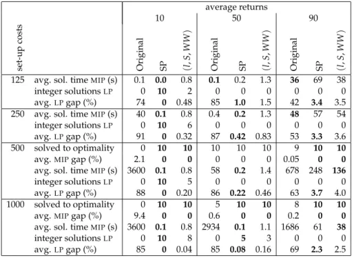
2.5 Computational tests . . . 32

2.5.1 Test set-up . . . 32

2.5.2 Results for the separate set-ups case . . . 32

2.5.3 Results for the joint set-ups case . . . 37

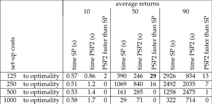
2.5.4 Comparison of SP and PSP2 . . . 38

3 The economic lot-sizing problem with an emission constraint 45 3.1 Introduction . . . 45 3.2 Problem definition . . . 49 3.3 Complexity results . . . 50 3.4 Structural properties . . . 53 3.5 Algorithms . . . 56 3.5.1 Lagrangian heuristic . . . 56

3.5.2 Pseudo-polynomial algorithm for co-behaving costs and emissions 59 3.5.3 FPTAS for co-behaving costs and emissions . . . 61

3.5.4 FPTAS for general costs and emissions . . . 64

3.5.5 Using the heuristic to speed up the FPTAS . . . 70

3.6 Computational tests . . . 72

3.6.1 Test set-up . . . 72

3.6.2 Results . . . 74

3.7 Conclusions & further research . . . 78

3.A Proof of Theorem 3.6 . . . 80

3.B Tables of results . . . 87

3.B.1 Results with improved lower bound . . . 87

3.B.2 Results without improved lower bound . . . 93

4 Lot-sizing with minimum batch sizes 99 4.1 Introduction . . . 99

4.1.1 Literature . . . 100

4.1.2 Outline . . . 103

4.2 Problem definition . . . 103

4.3 Structural properties . . . 106

4.3.1 Uncapacitated lot-sizing with minimum batch sizes . . . 106

4.3.2 Capacitated lot-sizing with minimum batch sizes . . . 111

4.4 Algorithms . . . 114

4.4.1 Uncapacitated lot-sizing with minimum batch sizes . . . 114

4.4.2 AnOT9_{algorithm for CLSMB . . . 117}

4.4.3 AnOT6_F−F_Lalgorithm for CLSMB . . . 122

4.5 Conclusion and discussion . . . 126

5 Summary of the main results 129 Nederlandse samenvatting (Summary in Dutch) 133

Contents xi

References 137

Chapter 1

Introduction

In this dissertation, green lot-sizing problems are studied. Before we proceed with the exposition of our research results in later chapters, we will answer two obvious questions:

1. What is a lot-sizing problem?

2. Why and how would such a problem be ‘green’?

1.1

Lot-sizing

The “dynamic version of the economic lot size problem”, which was introduced by Wagner and Whitin in their 1958 seminal paper, concerns a manufacturer who needs to solve a production planning problem. He is faced with a known, deterministic de-mand from his customers in a number of discrete time periods. The number of items demanded can vary over time. In each time period, he must decide to set up the pro-duction process or not, and if so how much to produce. If the propro-duction process is set up in a certain time period, he incurs fixed set-up costs. From this perspective, it would be cheapest to produce all items in the first time period and keep all of these items in inventory until they are demanded by the customers. However, in each time period, holding costs are incurred for each item that is held in inventory until the next period. From that perspective, he would like to produce each item in the same period as in which it is demanded, so that no item ever needs to be kept in inventory. Hence, there is a trade-off between set-up and holding costs. Per-unit production costs may also be incurred. The objective of the lot-sizing problem is to minimise the sum of all set-up, holding and production costs over all time periods, that is, over the entire

problem horizon. Solving the lot-sizing problem gives a production plan which pro-vides a production quantity for each time period, such that the aforementioned costs are minimised.

An alternative interpretation of the model is that of a firm that orders its prod-ucts from an (upstream) supplier. Setting up the production process in the description above then corresponds to placing an order at (or rather: receiving an order from) the supplier. If fixed ordering costs are associated with placing an order, then this prob-lem is mathematically equivalent and can also be described as a (dynamic) lot-sizing problem.

Mathematically, the classic (dynamic), single-item, uncapacitated lot-sizing prob-lem can be defined as a mixed integer linear program (MILP). First, we introduce the set of all time periods asT := {1, 2, . . . ,T}, whereTis the number of time periods. Next, we define three decision variables, for eacht∈ T:

xt is the quantity produced in time periodt;

yt is 1 if the production process is set-up in time periodt, and 0 otherwise;

It is the number of items carried in inventory from periodtto periodt+1.

Finally, we define the following parameters, again for eacht∈ T:

dt is the quantity demanded by customers in time periodt;

Kt are the fixed set-up costs in periodt;

pt are the per-unit production costs in periodt;

ht are the costs to hold one unit in inventory from periodtuntil periodt+1; M is a very large number; this number is typically defined as the sum of the

remain-ing demand until the end of the problem horizon;

T is the number of time periods, as mentioned before.

The classic lot-sizing problem is defined by the mixed integer program below.

min

∑

t∈T

(Ktyt+ptxt+htIt) (1.1)

s.t. It−1+xt = It+dt t∈ T (1.2)

1.1 Lot-sizing 3

1 2 3 4

I1 I2 I3

d1 d2 d3 d4

x1,y1 x2,y2 x3,y3 x4,y4

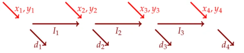
Figure 1.1:Graphical representation of a lot-sizing problem with four time periods

I0 = 0 (1.4)

xt,It ≥ 0 t∈ T (1.5)

yt ∈ {0, 1} t∈ T (1.6)

The objective (1.1) is to minimise the sum of all set-up, production and holding costs. Constraints (1.2) are inventory balance constraints. (1.3) are the so-called set-up forcing contraints. They make sure that the production quantity can only be strictly positive if there is a set-up in a period. Constraint (1.4) requires the initial inventory to be zero, which we can assume without loss of generality. Finally, (1.5) are the nonneg-ativity constraints, and constraints (1.6) impose that the set-up variables are binary.

Graphically, the classic lot-sizing problem can be represented as a network flow problem in the graph depicted in Figure 1.1. Here, theyts are binary variables,

indicat-ing whether there is a positive flow on an arc.

It is well-known that this classic lot-sizing problem is easy to solve. In their original paper, Wagner and Whitin (1958) solve this problem with dynamic programming in

OT2_{time, that is, the (worst-case) solution time is quadratic in the number of time}

periods. Their algorithm will even work if we generalise the production and holding costs to general concave functions, instead of the linear costs presented in the objec-tive function (1.1) above. For linear production and holding costs, the problem can be solved even faster, inO(TlogT)time, with the algorithms in Wagelmans et al. (1992), Aggarwal and Park (1993) and Federgruen and Tzur (1991). The same authors also show that the problem can be solved inO(T)time if the production and holding costs satisfy the Wagner-Whitin property. Such costs entail the absense of speculative mo-tives to hold inventory. This is mathematically defined aspt+ht≥ps∀t≤s∈ T.

The dynamic lot-sizing problem is well-studied in the literature and the classic problem has been extended in many different directions. Some of the most well-known extensions are the inclusion of production capacities (see e.g. Florian et al., 1980; Bitran and Yanasse, 1982; Van den Heuvel and Wagelmans, 2006), backlogging (see e.g. Zang-will, 1966; Pochet and Wolsey, 1988; Federgruen and Tzur, 1993) and batch-production

(see e.g. Lippman, 1969; Lee, 1989; Pochet and Wolsey, 1993; Constantino, 1998; Van Vyve, 2003 and Chapter 4 of this dissertation). For literature reviews of lot-sizing lems, see Jans and Degraeve (2007), who discuss metaheuristics for lot-sizing prob-lems, and Jans and Degraeve (2008), who discuss developments in the field of mod-elling industrial lot-sizing problems.

Extensions of the (classic) lot-sizing problem are also the topic of this dissertation. More specifically, we will concentrate on ‘green’ extensions, which take various envi-ronmental considerations into account.

1.2

Green

One of the definitions of the word ‘green’ in the Oxford English Dictionary is:

Of a product, service, etc.: designed, produced, or operating in a way that minimizes harm to the natural environment.

(Oxford English Dictionary Online, 2012, “green”, definition A.III.13.b). Minimising harm to the natural environment can of course be done in numerous ways. We will concentrate on two ways in this dissertation. Reducing the amount of pollutants that are emitted during the production process is one way. Another possibility is to re-duce the number of new products that need to be prore-duced, in other words: to rere-duce new material usage. This can be accomplished by reusing (parts of) a product after its initial use has ended. This implies that there is not only a forward flow of products, towards the customer/final user, but also a reverse flow, from the customer back one or more stages up the supply chain. By including a reverse flow in the supply chain, a loop is created, and the resulting system is appropriately called a closed-loop supply chain. The field of logistics that deals with this, is called reverse logistics. For litera-ture reviews, see Dekker et al. (2004), Souza (2013) and Guide and Van Wassenhove (2009). The literature can be classified in terms of strategic, tactical and operational issues. In this dissertation, we concentrate on the lot-sizing problem, which classifies as an operational model.

Within reverse logistics, we can distinguish between product reuse, remanufactur-ing and recyclremanufactur-ing. In conventional product reuse, an item is used again for the same function. Remanufacturing is a process where a particular product is taken apart, cleaned, repaired, and then reassembled to be used again. According to Thierry et al. (1995), ‘The purpose of remanufacturing is to bring used products up to quality stan-dards that are as rigorous as those for new products.’ In recycling, a used item is

1.3 Outline 5

broken down into raw materials that can be used to make new (and possibly different) products. In the first part of this dissertation, we will concentrate on remanufacturing items that are returned from users.

We will also concentrate on the amount of pollutants that are emitted during the production process. There are many pollutants; one could think of toxic waste, atmo-spheric particulate matter (such as soot and fine particles), and even smell, sound and light. In recent years, particular interest has been paid to the emission of greenhouse gases, such as carbon dioxide (CO2), nitrous oxide (N2O) and methane (CH4). By now,

there is a general consensus about the effect that these gases have on global warming. Consequently, many countries strive towards a reduction of these greenhouse gases, as formalised in treaties, such as the Kyoto Protocol (United Nations, 1998), as well as in legislation, of which the European Union Emissions Trading System (European Commission, 2010) is an important example. The shift towards a more environmen-tally friendly production process can be caused by such legal restrictions, but also by a company’s desire to pursue a ‘greener’ image by reducing its carbon footprint. As reverse logistics, the integration of carbon emission constraints can be considered at different decision levels: strategic, tactical and operational. Again, we will approach the emission problem from an operational point of view. We will consider various ways to incorporate emission reducing measures into lot-sizing models. The combina-tion of lot-sizing and carbon emissions has also been studied by Benjaafar et al. (2013) and Absi et al. (2013).

Finally, the environmental damage can be reduced by transporting items in a few larger shipments, rather than with many less-than-truckload shipments, or by produc-ing items in a few larger production batches, rather than many small batches. We will therefore also focus on imposing minimum batch sizes in lot-sizing problems.

1.3

Outline

This dissertation is organised around three themes: lot-sizing with remanufacturing, lot-sizing with an emission capacity constraint and lot-sizing with minimum batch sizes.

In Chapter 2, we consider lot-sizing problems in a remanufacturing context. In such a problem, new items can be produced as in any lot-sizing problem. However, in each time period, a certain quantity of used products is returned from customers. There is no demand for these returned products themselves, but they can be remanufactured, so that they become as good as new. Both newly produced items and remanufactured

returned items can then be used to fulfill customer demand. Production of new items and the remanufacturing of returned items can be carried out on one and the same pro-duction line or on separate ones. As such, we consider two variants of the lot-sizing problem with remanufacturing: one in which both processes have joint set-up costs and one in which there are separate set-up costs. We show that the variant with joint set-ups isN P-hard if the costs vary over time, and show that the variant with separate set-up costs isN P-hard even under time-invariant costs. For both variants, we present several mixed integer programming formulations. First, we give formulations based on ‘natural’ decision variables, corresponding to thext,ytandItvariables used in

Sec-tion 1.1. Next, we present formulaSec-tions that view the problem as several shortest path problems that are linked together. This type of formulation has got a larger number of decision variables than the natural formulation. Therefore, we will also present a par-tial shortest path formulation for the variant with separate set-ups. This is, in effect, a hybrid between the original formulation and the shortest paths formulation, which combines much of the smaller size of the natural formulation with the strength of a shortest path formulation. Each formulation is tested an a large number of problem in-stances, to find out which formulation performs best under which circumstances. The paper on which Chapter 2 is based, has been accepted for publication inIIE Tranactions

(Retel Helmrich et al., 2013).

Chapter 3 deals with lot-sizing with an emission capacity constraint. The model that we study can be seen as a classic lot-sizing problem with concave costs and a ‘second objective function’. As in the classic lot-sizing problem, we minimise the total costs over all periods (the ‘first’ objective function). The ‘costs’ in the second objec-tive function then refer to the emission levels of certain pollutants (for instance green-house gases, such as carbon dioxide) associated with production, keeping inventory and setting-up the production process. There is a strict constraint (a ‘cap’) on the sum of all emissions over all periods. As the ‘costs’ in this second objective function do not necessarily refer to emission levels, there is also a clear link with bi-objective optimisa-tion. Solving an instance of the lot-sizing problem with an emission capacity constraint corresponds to finding a specific point in the set of Pareto-optimal solutions. We will show that this problem isN P-hard and then propose several solution methods. First, we present a Lagrangian heuristic that provides both a feasible solution and a lower bound for the problem. For cost and emission functions that are such that the so-called zero-inventory (or single-sourcing) property is satisfied, we give an algorithm that runs in pseudo-polynomial time. This algorithm can also be used to identify the complete set of Pareto-optimal solutions of the bi-objective lot-sizing problem. Furthermore, we

1.3 Outline 7

develop a fully polyniomial time approximation scheme (FPTAS) for this problem and extend it to deal with general cost and emission functions. An FPTAS finds solutions to the problem that are arbitrarily (ε) close to the optimum and does so in a time that is polynomial in both the inverse precision (1/ε) and the size of the problem instance. We also explain how we can use the results of the Lagrangian heuristic to kick-start the FPTAS. Finally, extensive computational tests give detailed insights into both the com-putation time and the quality of the obtained solutions of the various algorithms. An ealier version of Chapter 3 has appeared as working paper Retel Helmrich et al. (2011). The paper on which this chapter is based is currently under review for publication in

theEuropean Journal of Operational Research.

In Chapter 4, we consider a lot-sizing problem in which production takes place in batches. These batches have a certain (nonzero) minimum and maximum size. More than one batch can be produced in one production period, but there may also be a ca-pacity constraint on the number of batches that can be produced in one period. We will consider both variants in this chapter. Although it might not be clear at first glance, this problem is also clearly related to green production planning. A retailer, for instance, may procure its inventory from an external supplier. A popular strategy like just-in-time ordering will often lead to very frequent small shipments from the supplier to the retailer, resulting in high levels of carbon emissions. By imposing a minimum on the size of a shipment, or batch, in each period, we prevent products from being trans-ported by almost empty vehicles, or machines from producing only very few units of a product per batch. The latter will reduce the number of times the production pro-cess has to be set up, along with the associated pollution. We present several dynamic programming algorithms that solve both the capacitated and uncapacitated variant of this problem in polynomial time in the case that the costs satisfy the Wagner-Whitin property, as described in Section 1.1.

Chapter 2

Economic lot-sizing with

remanufacturing: complexity and

efficient formulations

Abstract

Within the framework of reverse logistics, the classic economic lot-sizing problem has been ex-tended with a remanufacturing option. In this exex-tended problem, known quantities of used products are returned from customers in each time period. These returned products can be remanufactured, so that they are as good as new. Customer demand can then be fulfilled both from newly produced and remanufactured items. In each period, we can choose to set up a process to remanufacture returned products or produce new items. These processes can have separate or joint set-up costs. In this chapter, we show that both variants areN P-hard. Further-more, we propose and compare several alternativeMIPformulations of both problems. Because ‘natural’ lot-sizing formulations provide weak lower bounds, we propose tighter formulations, namely shortest path formulations, a partial shortest path formulation and an adaptation of the(l,S,WW)-inequalities for the classic problem with Wagner-Whitin costs. We test their ef-ficiency on a large number of test data sets and find that, for both problem variants, a (partial) shortest path type formulation performs better than the natural formulation, in terms of both theLPrelaxation andMIPcomputation times. Moreover, this improvement can be substantial.

2.1

Introduction

Reverse logistics (see Dekker et al., 2004) is a field that has emerged during the last decades. It studies situations in which there is not only a product flow towards the

customers, but products and materials are also returned to the manufacturer and these may be reused in production processes. Remanufacturing is a process where a par-ticular product is taken apart, cleaned, repaired, and then reassembled to be used again. According to Thierry et al. (1995), ‘The purpose of remanufacturing is to bring used products up to quality standards that are as rigorous as those for new products.’ The importance of remanufacturing is underlined by the fact that remanufacturing has been included in many MRP (II), and later ERP, systems for years; see e.g. Ferrer and Whybark (2001), Ptak and Schragenheim (2000), De Brito (2004), and Fargher (1997). A (re-) manufacturer uses such a system to plan its (re-) manufacturing operations. Examples of commercial ERP systems that provide the option to incorporate remanu-facturing operations are SAP and JD Edwards EnterpriseOne (see SAP, 2012a; Oracle, 2012). Moreover, it is possible in SAP to substitute a newly produced for a remanufac-tured product, as we will do in this chapter.

In this chapter, we concentrate on mixed integer programming (MIP) formulations. These mixed integer programs provide a general framework that can be easily ex-tended and adapted by practitioners or other researchers, for instance with side con-straints or additional variables. Within the framework of reverse logistics, we focus on the classic economic lot-sizing problem that has been extended with a remanufacturing option. This arises as a (sub-) problem in MRP.

As in the classic problem, we face a deterministic demand from customers in a number of discrete time periods. In each period, we must decide to set up a production process or not, and if so how much to produce. In order to find a production plan with minimal costs, we must find the optimal balance between set-up, holding and production costs. In the problem extended with a remanufacturing option, known quantities of used products are returned from customers in each period. There is no demand for these returned products themselves (or ‘returns’ in short), but they can be remanufactured, so that they are as good as new. Customer demand can then be fulfilled from two sources, namely newly produced and remanufactured items. Since both can be used to serve customers, they are referred to as ‘serviceables’. We are to determine in which periods to set up a production process to remanufacture returned products and in which to set up a production process to manufacture new items. Thus, the traditional trade-off between set-up, holding and production costs is extended with remanufacturing costs and holding costs for returns.

After showing that the economic lot-sizing problem with remanufacturing isN P -hard, we shall propose several alternative formulations. Computational tests show that these improved formulations have better LP relaxations and MIP computation

2.1 Introduction 11

times compared to standard lot-sizing formulations as in Teunter et al. (2006). More-over, the general framework proposed in this chapter can be used to solve larger, com-plex problems that could not be solved before.

Next, we will discuss in detail the two major assumptions that are present in our model, namely the deterministic demand and return flow, and the as-good-as-new quality of the remanufactured products. When using this model, it is important that one verifies whether these assumptions hold in practice, as they do not apply to each setting.

The first major assumption is that both demand and returns are deterministic. As we mentioned before, remanufacturing has been included in many MRP and ERP sys-tems for years and (re-) manufacturers use such a system to plan their (re-) manu-facturing operations. In general, these systems require the solution of deterministic production planning problems. Moreover, Gotzel and Inderfurth (2002) find that ‘the application of an MRP-based approach to the production/remanufacturing problem is promising, even in case of multiple stochastic influences.’ In their approach, they make several adjustments to the control parameters, to deal with various degrees of uncertainty. Thus, we see that in this case a deterministic model as in MRP can still be a good approximation if there is uncertainty. As Pochet and Wolsey (2006) men-tion, MRP/ERP systems use heuristics to solve their planning problems (see also SAP, 2012b). As these generally lead to suboptimal production plans, it would be worth-while to investigate how to solve such problems optimally in an efficient (fast) way.

Examples of prior literature in which deterministic returns are considered an ap-propriate approximation, are Golany et al. (2001) and Beltr´an and Krass (2002), who give examples of practical situations to which their model with deterministic returns can be applied. Golany et al. (2001) mention that the demand for and returns of pack-aging and shipping materials (such as pallets or containers) are known, since the ship-ments in which they are used, are planned in advance. Beltr´an and Krass (2002) discuss catalogue retailing, in which ‘the proportion of each period’s sales that come back as returns, and the timing of these returns are often quite stable (. . . ) making it possible to forecast returns in each period quite accurately’.

Although we have seen that certain stochastic settings can be captured by a deter-ministic model, we do acknowledge that the assumption of deterdeter-ministic demand and returns can be too strong in certain situations. However, we have seen that the same assumption is used when solving production planning problems in ERP systems.

The second major assumption is that demand may be satisfied by either new or re-manfactured products. That is, we assume that remanufactured products are as good

as new. Guide and Li (2010) have done experiments that show that, especially for consumer products, ‘consumers of the new and the remanufactured products are seg-mented, and therefore, cannibalization is not a significant managerial concern.’ On the other hand, they indicate that there may be a certain degree of cannibalization in the business to business (B2B) market.

Moreover, customers are not always offered a choice between the remanufactured and newly manufactured version of a product, and may be unaware of this difference altogether. Examples include single-use camera’s and printer cartridges. For Kodak’s single-use cameras, Guide and Van Wassenhove (2002) mention that ‘The final product containing remanufactured parts and recycled materials is indistinguishable to con-sumers from single use cameras containing no reused parts.’ About Xerox printer cartridges, the same authors write that ‘The final cartridge product containing reman-ufactured parts or recycled materials is indistinguishable from cartridges containing exclusively virgin materials.’ Moreover, as part of its ‘Green World Alliance’, Xerox says (in Xerox, 2010a, see also Xerox, 2010b) : ‘On average, approximately 60% by vol-ume of the used cartridges returned to Xerox are remanufactured. Remanufactured cartridges, containing an average of 90% reused/recycled parts, are built and tested to the same performance specifications as new products.’

Futhermore, all demand that a company faces may be internal, i.e. the company needs the products itself. As such, we can know for sure that the ‘end-users’ are in-different between the remanufactured and newly manufactured product. For instance, this can be the case with packaging materials, such as pallets or containers, as Golany et al. (2001) mention. Of course, many such packaging materials are reused, rather than remanufactured, but, in this chapter, the term ‘remanufacturing’ also applies to

reusableproducts that simply need to be cleaned or transported to another location.

Finally, demand may be satisfied from both sources, when customers do not actu-ally buy a specific physical product, but have a service contract. Thierry et al. (1995) give a good example of this for ‘Copy magic’, a multinational copier manufacturer. They write: ‘Since the quality of the remanufactured products is ”as good as new,” these products are treated in the same way as new products: similar warranties, sim-ilar service contracts. Lease prices for both product categories are identical.’ They do mention that many marketing efforts were needed to convince customers that remanu-factured products are indeed as good as new, and that selling prices of remanuremanu-factured products are somewhat lower than those of new products.

As in Teunter et al. (2006), we consider two variants of lot-sizing with remanufac-turing. In the first variant, manufacturing new products and remanufacturing used

2.1 Introduction 13

products take place in two separate processes, each with its own set-up costs. We call this problem ELSRs (Economic Lot-Sizing with Remanufacturing and Separate set-ups). In the second variant, the manufacturing and remanufacturing process have one joint set-up cost, for instance because manufacturing and remanufacturing operations are performed on the same production line. We call this problem ELSRj (Economic Lot-Sizing with Remanufacturing and Joint set-ups).

ELSRj with time-invariant costs can be solved inO(T4)time with the dynamic pro-gramming algorithm proposed in Teunter et al. (2006). However, in this chapter we will show that ELSRj isN P-hard in general. Moreover, we will prove that ELSRs is

N P-hard even if all costs are time-invariant.

Because of their complexity, it makes sense to look at good mixed integer program-ming (MIP) formulations of both problems, which is what we do in this chapter. A first formulation with a ‘natural’ choice of variables was presented in Teunter et al. (2006) and will serve as our benchmark. We shall see, however, that such a formulation con-tains so-called ‘big M’ constraints. It is generally known (Pochet and Wolsey, 2006) that these big Mconstraints in the natural lot-sizing formulation often lead to a bad

LP-relaxation and hence high running times. Consequently, we propose several new, alternative formulations of the lot-sizing problem with remanufacturing. The first re-formulation is based on a shortest path type re-formulation, as first proposed by Eppen and Martin (1987) for the capacitated lot-sizing problem (without remanufacturing). The second reformulation is a partial shortest path reformulation. This reformula-tion has fewer variables than the full shortest path reformulareformula-tion, while preserving the quality of theLP-relaxation as much as possible. This idea was used by Van Vyve and Wolsey (2006) for the classic lot-sizing problem. The last formulation is based on the

(l,S,WW)-inequalities, as introduced by Pochet and Wolsey (1994) for the single-item uncapacitated lot-sizing problem with Wagner-Whitin costs. In order to assess and compare their performances, we will subject all the formulations to a large number of computational tests.

To the best of our knowledge, no-one has ever presented and tested a goodMIP for-mulation for the economic lot-sizing problem with remanufacturing. Previous work generally used heuristics or solved restricted versions of the problem. Van den Heuvel (2006) solves ELSRs with a genetic algorithm that uses dynamic programming to solve subproblems in which the production periods are given. Teunter et al. (2006) present heuristics for both ELSRs and ELSRj. These heuristics are modifications of the well-known Silver-Meal, Least Unit Cost and Part Period Balancing heuristics (see Silver et al., 1998). Recently, Schulz (2011) proposed an improvement of the modified

Silver-Meal heuristic for ELSRs. Exact dynamic programming algorithms were developed by Pan et al. (2009) for several special cases of the capacitated lot-sizing problem with production, disposal and remanufacturing. This includes lot-sizing with uncapaci-tated production and capaciuncapaci-tated remanufacturing and no final inventory of returns, for which their algorithm runs in exponential time. With this algorithm, they solve in-stances with up to 14 periods. Richter and Sombrutzki (2000) study a ‘reverse Wagner-Whitin model’ with time-invariant costs in which there is an abundance of returns. As such, manufacturing items is not necessary, but may result in a production plan with lower costs. The problem is solved with an algorithm similar to Wagner and Whitin’s. This model and algorithm are extended in Richter and Weber (2001) with variable (re-) manufacturing costs. In the case of time-invariant costs and demand inputs, they find an ‘optimal switching point’ between remanufacturing and manufacturing. Golany et al. (2001) study the lot-sizing problem with remanufacturing in which it is possible to dispose returned products. They show that the problem isN P-hard for general con-cave costs, but solvable as a transportation problem inO(T3)time if all costs are linear. The same setting is studied in Yang et al. (2005). They extend theN P-hardness result to the time-invariant costs case and develop a heuristic that runs in polynomial time. Pi ˜neyro and Viera (2009) study a similar model with a disposal option, but the concave costs are restricted to fixed-plus-linear costs for (re-) manufacturing and disposing, and holding costs are assumed linear. They construct a tabu search procedure for this prob-lem, as well as several inventory policies that run inO(T2)time. Beltr´an and Krass (2002) also consider a setting where disposal of returns is possible, but they assume that remanufacturing returned items is not necessary, i.e. returns can directly be used to satisfy demand. For this setting, they develop a dynamic programming algorithm that runs inO(T3)time. Finally, Zhou et al. (2011) study a single-product, periodic-review inventory system with multiple types of returned products. Both newly man-ufactured and remanman-ufactured products can be used to fulfill stochastic demand, and the objective is to minimize the expected total discounted costs over a finite planning horizon.

The remainder of this chapter is organized as follows. The next section presents a formal definition of ELSRs and ELSRj by giving a first, ‘natural’MIPformulation. In Section 2.3, we show that both ELSRs and ELSRj areN P-hard in general. All of our reformulations are presented in Section 2.4. These formulations are put to the test in Section 2.5 and Section 2.6 concludes this chapter, with some suggestions for further research.

2.2 The original formulation 15

2.2

The original formulation

2.2.1

Separate set-ups

We can formulate the lot-sizing problem with remanufacturing as a mixed integer pro-gram. A first, ‘natural’ formulation is based on the following decision variables:

xm_t is the number of items manufactured in periodt;

xr

t is the number of items remanufactured in periodt;

ym_t is 1 if the manufacturing process is set up in periodt; 0 otherwise;

yr

t is 1 if the remanufacturing process is set up in periodt; 0 otherwise; I_ts is the inventory of serviceables at the end of periodt;

I_tr is the inventory of returns at the end of periodt.

The notation that is used for the parameters in each periodt, is as follows:

dt is the customer demand, whereDi,j:=∑jt=idt; rt is the amount of returns, whereRi,j:=∑tj=irt;

hs_tandhr_t are the unit holding costs for serviceables and returns, respectively;

Km

t andKrt are the set-up costs for manufacturing and remanufacturing,

respec-tively;

pm_t andpr_t are the unit production costs for manufacturing and remanufacturing, respectively.

A network flow representation of this problem and its variables and parameters is given in Figure 2.1.

We are now ready to present a first, ‘natural’ formulation of the lot-sizing problem with remanufacturing and separate set-ups. This formulation is similar to the ones in Teunter et al. (2006), Yang et al. (2005) and Pi ˜neyro and Viera (2009), and will serve as our benchmark. min T

∑

I₁s I₂s I₃s Ir 1 I2r I3r d1 d2 d3 d4 r1 r2 r3 r4 Ir 4 xm₁,y₁m xm₂,ym₂ xm₃,ym₃ xm₄,ym₄ xr 1yr1 xr2yr2 x3r yr3 x4r yr4

Figure 2.1:Network flow representation of ELSRs s.t. I_ts = I_ts₋₁+x_tm+xr_t−dt t=1, . . . ,T (2.2) I_tr = I_tr₋₁−xr_t+rt t=1, . . . ,T (2.3) xm_t ≤ Dt,Tymt t=1, . . . ,T (2.4) xr_t ≤ D_t,Tyrt t=1, . . . ,T (2.5) xm_t,xr_t,I_ts,I_tr ≥ 0 t=1, . . . ,T (2.6) ym_t,yr_t ∈ {0, 1} t=1, . . . ,T (2.7) I₀s=I₀r = 0 (2.8)

We shall refer to this formulation as ‘Original’. It also serves as our (formal) defini-tion of the economic lot-sizing problem with remanufacturing and separate set-ups (ELSRs).

The objective (2.1) is to minimise the sum of set-up costs of the production and remanufacturing processes, production and remanufacturing costs, and holding costs for serviceables and returns. (2.2) and (2.3) are inventory balance constraints for ser-viceables and returns, respectively. (2.4) and (2.5) are set-up forcing constraints for the manufacturing and remanufacturing processes. The last constraints (2.8) assume zero initial inventories of both serviceables and returns, without loss of generality.

2.2.2

Joint set-ups

For the problem variant with joint set-ups, we give a similar formulation. The notation is the same as before, but now we have only one set-up variable,yt, and one parameter

2.3 Complexity results 17

to denote the set-up costs,Kt.

min T

∑

We shall also refer to this formulation as ‘Original’. As before, it serves as our (formal) definition of the economic lot-sizing problem with remanufacturing and joint set-ups (ELSRj). The interpretation of the formulation is similar to the separate set-ups case.

2.3

Complexity results

2.3.1

Lot-sizing with remanufacturing and separate set-ups

Richter and Sombrutzki (2000) and Richter and Weber (2001) show that some special cases of the ELSRs problem can be solved in polynomial time. However, Richter and Sombrutzki (2000, p. 311) mention that “There are probably no simple algorithms to solve that general model . . .”. In this section, we will show that the ELSRs problem is indeedN P-hard in general. In the proof, we will use a reduction from the well-known

N P-completePARTITIONproblem (see problem [SP12] in Garey and Johnson (1979)). ProblemPARTITION: Givennpositive integersa1, . . . ,an, does there exist a setS⊂N= {1, . . . ,n}such that_∑i∈Sai =∑i∈N\Sai=A? (Note that we may assume without loss

of generality thata_i<Afori=1, . . . ,n.)

Theorem 2.1. The ELSRs problem isN P-hard for time-invariant cost parameters.

Proof. Given an instance ofPARTITION, we construct an instance of the ELSRs problem

withT = nperiods as follows. Fort = 1, . . . ,T, letdt = at,Kmt = Krt = 1,pmt = 1, pr_t = 0, hs_t = 3 and hr_t = 0. Furthermore, letr1 = A and rt = 0 fort = 2, . . . ,T.

toPARTITIONis positive if and only if the ELSRs instance has a solution with a cost of at mostT+A.

Assume that we have a solution for the ELSRs instance with a cost of at mostT+A. First, we show that we may restrict ourselves to a solution where no serviceables are held in stock. To that end, lettbe the first period with serviceables in stock, so thatt

is a manufacturing or remanufacturing period. Now decreasing the number of items being (re)manufactured by one in periodtand increasing the number of items being (re)manufactured by one in periodt+1 will reduce the total cost by at least 1. By repeating this process we end up with a solution without serviceables in stock and cost at mostT+A.

Because at mostAitems can be remanufactured and all demand has to be satisfied, we incur at least a variable cost of Afor manufactured items and this cost is exactly

Aif all returns are remanufactured. Moreover, since no serviceables are held in stock and demand is positive, every period is a manufacturing or remanufacturing period. So if there is both remanufacturing and manufacturing in at least one period, then the total setup costs will exceedT. Because the total cost is at mostT+A, the total amount remanufactured equals A and demand in each period is satisfied by either manufacturing or remanufacturing (and not both). Therefore, the remanufacturing periods (or the manufacturing periods) form the setS.

Conversely, letSbe the set for which_∑i∈Sa_i =_∑i∈N\Sa_i = A. It is easy to verify that by remanufacturingatitems in each periodt ∈Sand manufacturingatitems in

each periodt∈N\S, all demand is satisfied and total costs equalT+A.

Note that from a practical point of view, the ELSRs problem instance in the proof has reasonable assumptions on the cost parameters. Since remanufacturing adds value to an item, it is reasonable to assume that holding serviceables is at least as costly as holding returns (i.e.hs_t ≥hr_t). Furthermore, if remanufacturing is motivated econom-ically, then the assumption that the unit remanufacturing cost equals at most the unit manufacturing cost (i.e. pm

t ≥ prt) is also reasonable. Finally, in practice it is likely

that the total amount of demand will be larger than the total amount of returns (i.e.

∑T

t=1dt≥∑Tt=1rt).

Note that the solution for thePARTITIONinstance and the optimal cost of the EL-SRs instance are independent of the ordering ofa1, . . . ,an(as in theN P-completeness

proof for the capacitated lot-sizing problem (Florian et al., 1980)). This gives the fol-lowing corollary:

2.3 Complexity results 19

Corollary 2.2.The ELSRs problem remainsN P-hard in the case of increasing (or decreasing) demand over time and time-invariant cost parameters.

2.3.2

Lot-sizing with remanufacturing and joint set-ups

Although the lot-sizing problem with remanufacturing and joint set-ups can be solved inO(T4_{)time with the algorithm presented in Teunter et al. (2006) when all costs are}

time-invariant, we show that ELSRj isN P-hard in general.

Theorem 2.3. The ELSRj problem isN P-hard.

Proof. We show that the lot-sizing problem with remanufacturing and separate set-ups

is a special case of the problem with joint set-ups. Let an instance of ELSRs be defined as in (2.1)–(2.8). We define an instance of the lot-sizing problem with remanufacturing and joint set-ups as follows:

˜ T = 2T K˜t = K_tr fortodd Km t forteven ˜ dt = 0 fortodd d1 2t forteven ˜ rt = r1 2(t+1) fortodd 0 forteven ˜ pm t = ⎧ ⎨ ⎩ ∞ fortodd pm 1 2t forteven p˜rt = ⎧ ⎨ ⎩ pr1 2(t+1) fortodd ∞ forteven ˜ hs_t = ⎧ ⎨ ⎩ 0 fortodd hs1 2t forteven h˜ r t = ⎧ ⎨ ⎩ 0 fortodd hr1 2t forteven

Note that the parameters with tilde correspond to ELSRj, whereas the ones without correspond to ELSRs. An illustration of such an instance of ELSRj can be found in Figure 2.2. Since this problem has joint set-up costs, there is a common fixed charge (Kr₁,K₁m,Kr₂,Km₂, . . .) on twoarcs in each period. Observe that each periodtin ELSRs corresponds to a two-period pair (2t−1, 2t) in ELSRj. In the first period of such a two-period pair, the returned products become available and in the second customer demand takes place. Inventory of both serviceables and returns can be carried between two such periods without costs. Furthermore, remanufacturing will only take place in the first and manufacturing only in the second period. In accordance with this, we have chosen ˜K2t−1 = Ktrand ˜K2t =Kmt. Since all other parameters in the instance of

ELSRj correspond directly to their counterparts in ELSRs, it is easy to see that ELSRs is indeed a special case of ELSRj. Since this reduction can clearly be performed in polynomial time, it follows that Theorem 2.3 holds.

0 hs 1 0 h2s 0 hr 1 0 hr2 d1 d2 r1 r2 ∞,K₁r pm₁,K₁m ∞,K₂r pm₂,K₂m pr 1 K1r ∞ Km1 pr3 K2r ∞ Km2

Figure 2.2:ELSRs as a special case of ELSRj

We can show that both ELSRj and ELSRs areN P-hard in the weak sense. It is easy to find a pseudo-polynomial algorithm for ELSRj, based on the following recursion:

g(t,Ir_t−1,I_ts₋₁) =min Ir t,Its c(t,I_tr₋₁,I_ts₋₁,I_tr,I_ts) +g(t+1,I_tr,I_ts) , where g(T+1,Ir

T,ITs) = 0. Here,g(t,Itr−1,Its−1)gives the total costs in periodtuntil

the end of the horizon (T), given the starting inventories of serviceables and returns in periodt. Clearly,g(1, 0, 0)gives the optimal value of an instance of our problem. Furthermore,c(t,Ir

t−1,Ist−1,Itr,Its)are the total costs in periodt. Given the starting and

ending inventories of serviceables and returns, we know exactly how much to manu-facture and remanumanu-facture in periodt, and these costs are easy to compute. There are

O(TR1TD1T)states ofg, and we need to optimize overO(R1TD1T)values to compute

oneg(t,I_tr₋₁,I_ts₋₁). Thus, the optimum can be found inOT(D1TR1T)2

time, which is pseudo-polynomial. Moreover, we have shown that ELSRs is a special case of ELSRj (see Theorem 2.3), so both ELSRj and ELSRs are weakly NP-hard.

2.4

Reformulations

In equations (2.2)–(2.8), we can see that the natural formulation contains two ‘bigM’ type constraints. It is generally known that these bigMset-up constraints in lot-sizing often lead to a badLPrelaxation (Pochet and Wolsey, 2006). In order to obtain better lower bounds, we propose several alternative formulations of the lot-sizing problem with remanufacturing, namely a shortest path reformulation (in Section 2.4.1), a partial

2.4 Reformulations 21

shortest path reformulation (in Section 2.4.2) and a formulation that uses an adaptation of the(l,S,WW)inequalities (in Section 2.4.3).

2.4.1

The shortest path reformulation

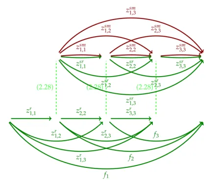
The formulation presented in this section is based on a shortest path reformulation, as proposed by Eppen and Martin (1987) for the capacitated lot-sizing problem. They solved a shortest path problem in a network with flow variables zi,j (where i ≤ j)

through which a unit flow is sent. For three periods, this network corresponds to (only) thezsm

i,j variables in Figure 2.3. An example of a feasible solution in this network

is z1,2 = 1₃,z1,3 = 2₃, z3,3 = 1₃, andzi,j = 0 otherwise. This means that in period

1, we produce 1₃ of the demand in periods 1 and 2, and 2₃ of the demand in periods 1, 2 and 3. In other words: all demand in periods 1 and 2, and 2₃ of the demand in period 3 are satisfied by items produced in the first period. Finally, the remaining 1₃ of the demand in period 3 is produced in period 3 itself. Notice that we start with a flow of one at the first node and that in each node the inflow equals the outflow. In our example, we have a set-up in periods 1 and 3, and this corresponds exactly to the nodes with a nonzero outflow. Moreover, observe that in each periodi, we can compute the production quantities as x_i = _∑T_t=iD_i,tz_i,t. Using this relation between the x and z

variables, the production and holding costs on each arczi,jcan be computed exactly.

For the classic (single-item uncapacitated) lot-sizing problem, theLPrelaxation of the shortest path formulation always gives an integer solution, i.e. the optimal solution of the classic lot-sizing problem. The problem with remanufacturing can be viewed as having two products: serviceables and returns. A shortest path type reformulation can be applied to both.

Separate set-ups

When formulating the layer of serviceables as a shortest path problem, one should note that there are two sources from which demand can be fulfilled, newly produced and remanufactured products. Because both production processes have separate set-up costs (and hence separate binary variables,ym_t andyr_t), we also need two types of flow variables (as opposed to one in Eppen and Martin’s original shortest path refor-mulation). Call these flow variableszsm

i,j and zsri,j. Here, zsmi,j is defined as the fraction

of demand ineachof the periodsiuntiljthat is fulfilled by newly produced items in periodi. Similarly,zsr

i,jis defined as the fraction of demand ineachof the periodsiuntil jthat is fulfilled by items that are remanufactured in periodi.

(2.28) (2.28) (2.28) z_1,1sm zsm 2,2 zsm3,3 zsm 1,2 zsm2,3 zsm 1,3 zsr 1,1 zsr2,2 zsr3,3 z_1,2sr zsr_2,3 zsr_1,3 zr_1,1 zr_2,2 zr_3,3 zr_1,2 z_2,3r f3 zr_1,3 f2 f1

Figure 2.3:The shortest path reformulation

When formulating the layer of returns as a shortest path problem, one should note that this is exactly the classic lot-sizing problem, but with the time reversed. In the classical case, production in some periodtis used to satisfy given demand in future periodst,t+1, . . .. Here however, there is a given amount of returns in each period that is remanufactured in some future periodt. The variablezr

i,jis defined as the

frac-tion of returns ineachof the periodsiuntiljthat is remanufactured in periodj. This formulation also provides the opportunity to have a final inventory of returns, i.e. not all returns need to be remanufactured within the problem horizon. For this purpose, defineft(t∈ {1, . . . ,T}) as the fraction of returns ineachof the periodstuntilTthat is

added to the final inventory of returns at the end of periodT. Following this definition, we can say thatIr

T =∑tT=1Rt,Tft. A shortest path reformulation with three periods is

depicted in the graph in Figure 2.3.

Before giving the objective function and constraints, we define the following cost parameters.

2.4 Reformulations 23 Csm_i,j = pm_i Di,j+ j−1

∑

∑

∑

∑

i,j are the total variable production plus holding costs of solely using new

pro-duction in periodito satisfy demand in periodsi,i+1, . . . ,j. Similarly, if demand in periodsi,i+1, . . . ,jis solely satisfied by products that are remanufactured in period

i, thenCsr

i,jare the total variable remanufacturing costs plus the holding costs that are

incurred from the moment these products are remanufactured until they are used to satisfy demand. Furthermore, if all returns in periodsi,i+1, . . . ,jare remanufactured in period j, then Cr

i,j are the total holding costs that are incurred from the moment

these returns become available until they are remanufactured. Finally,C_tf are the costs of holding all returns in periodst,t+1, . . . ,Tin inventory until the end of the problem horizon (without remanufacturing them), wherehr

Tmay denote the variable costs of

final disposal of returns (at the end of the problem horizon).

We are now ready to present our shortest path formulation (SP) of ELSRs.

min T

∑

_∑

∑

∑

∑

∑

∑

∑