Enumeration of weighted games with minimum and an analysis of voting power for bipartite complete games with minimum

Enumeration of weighted games with minimum and an

analysis of voting power for bipartite complete games

with minimum

Josep Freixas

Sascha Kurz

Abstract

This paper is a twofold contribution. First, it contributes to the problem of enumer-ating some classes of simple games and in particular provides the number of weighted games with minimum and the number of weighted games for the dual class as well. Second, we focus on the special case of bipartite complete games with minimum, and we compare and rank these games according to the behavior of some efficient power in-dices of players of type 1 (or of type 2). The main result of this second part establishes all allowable rankings of these games when the Shapley-Shubik power index is used on players of type 1.

Key words: simple game; weighted and complete games; enumerations; Shapley-Shubik power index; Banzhaf power indices.

Math. Subj. Class. (2000): Primary 91A12, 91A40, 91A80, 91B12. JEL Class.: C71, D71.

1

Introduction

The study of voting systems can be traced back to the late nineteenth century, when Dedekind studied monotonic Boolean functions. In the context of voting systems these functions correspond to simple games. In their seminal book, von Neumann and Morgen-stern [34] came up with the definition of a simple game as a type of cooperative game where the payoffs to coalitions are either 1 or 0, i.e., coalitions can be considered either winning or losing.

∗_{Department of Applied Mathematics III and High Engineering School (Manresa Campus), Technical}

University of Catalonia (Spain). e–mail: [email protected]. Research partially funded by Grants SGR 2009–1029 ofGeneralitat de Catalunyaand MTM 2012–34426 from the Spanish Economy and Competitive-ness Ministry, from the Spanish Science and Innovation Ministry. E-mail: [email protected]

†_{Department of Mathematics, Physics and Computer Science, University of Bayreuth, 95440 Bayreuth,}

A particular case of simple games, and possibly the most important subcase, is that of weighted games, in which weights are assigned to players and a threshold is set so that a coalition is winning if and only if the sum of weights of its players is at least the threshold. This is natural in Parliaments and also in corporate voting when different shareholders may own different numbers of shares. Two natural extensions of weighted games have also been thoroughly studied: (1) complete games and (2) simple games with small dimension. In this paper we deal with a particular class of complete games, the so called “complete games with minimum” (see, e.g., [17] and [18]).

It turns out that every complete game with five or fewer players is weighted, so the small-est possible illustrations of complete non-weighted games occur for six players: y1, y2, b1, b2, b3,

andb4 (herey means players of yellow type, whereasbmeans players of blue type), and we

declare that a coalition is winning if and only if it contains: at least three players and at least one of them is yellow. Intuitively, it is clear that all the yellow players have the same influence (according to the desirability relation), and all the blue players have the same influence, but the yellow players have more influence than the blue players –suggesting a complete (weak) ordering for the players in this example of a voting system. In terms of the language we introduce later (in Section 2) this simple game is complete but not weighted.

Note that e.g., the coalitions of type {y1, y2, bi} for i = 1,2,3,4 are minimal winning

since all players contained are essential for the coalition to be winning. The same occurs for the coalitions {yi, bj, bk} for i = 1,2 and 1 ≤ j < k ≤ 4. However, this latter set

of coalitions has an additional singularity: none of the players in these coalitions can be replaced by a weaker player. E.g., we cannot replace in these coalitions the yellow player for a blue player since the new coalition obtained would not be winning. In terms of the language we introduce later (in Section 2) we say that the coalitions of type{yi, bj, bk}for

i = 1,2 and 1≤j < k ≤ 4 are shift-minimal winning coalitions. On the contrary, if in a shift-minimal winning coalition we replace a weaker player by a stronger one we obtain a minimal, but not shift-minimal, winning coalition. Finally, observe that all shift-minimal winning coalitions have the same number of players of each color, i.e., they all contain one yellow player and two blue players and this information can be encapsulated in the vector: (1,2) where the first component represents the number of yellow players and the second the number of blue players. Then, we refer to the game as being complete with only one type of shift-minimal winning coalitions, or equivalently, a complete game with minimum as was denominated in [17] and [18]. Note that in the previous example there is a bipartition between types of players: yellow players and blue players. Hence, the example introduced is a bipartite complete game with minimum.

The first part of the paper deals with enumerations for weighted games with minimum, while the second part deals with rankings of players for power indices in bipartite complete games with minimum. The dimension of complete games with minimum is studied in [18]. For instance, the previous example has dimension 2 and, therefore, it decomposes as the intersection of two weighted games: [5; 3,3,1,1,1,1]∩[3; 1,1,1,1,1,1] (the notation for a representation of a weighted game is introduced in the preliminaries section). Most existing voting systems have a small dimension. E.g., the current voting system of the European Council is an example of a complete game with dimension 3, i.e., it decomposes as an intersection of three weighted games which cannot be simplified to an intersection of fewer

weighted games [12].

The voting system to amend the Canadian Constitution is an example of a non-weighted game which meets both requirements: it is complete (and has only one type of shift-minimal winning coalitions) and has dimension 2, i.e., it decomposes as the intersection of two weighted games. Since 1982, an amendment to the Canadian Constitution can become law only if it is approved by at least seven of the ten Canadian provinces, subject to the pro-viso that the approving provinces have, among them, at least half of Canada’s population. It was first studied in Kilgour [23]. A census (in percentages) taken from 1960 for the Cana-dian provinces was: Prince Edward Island (1%), Newfoundland (3%), New Brunswick (3%), Nova Scotia (4%), Manitoba (5%), Saskatchewan (5%), Alberta (7%), British Columbia (9%), Quebec (29%) and Ontario (34%). This is another example of a bipartite complete game with minimum and the vector representing all shift-minimal winning coalitions is: (1,6) where the first component indicates that exactly one of the two most populated provinces votes in favor of the voted law and 6-out-of-8 of the other provinces vote in favor of the voted law as well. Games of this type are the object of study in this paper.

This paper primarily concerns enumerations. The number of complete games is known up to nine players only [14], and the number of weighted games is also known up to nine players [26]. A seminal result on enumeration formulas for weighted games and complete games is May’s theorem [31], and many other results have followed, e.g., the enumeration of weighted games with up to six players dates back at least to 1962 [33].

The mathematical structure of complete games was studied in detail in the nineties by several scholars, e.g., in [25] and [4]. In the latter work a system of quantities (called characteristic invariants) is associated with every complete game and their basic properties are stated. It is shown that these quantities determine the game (uniqueness) and that every such system is associated with some complete game (existence).

According to this classification the simplest case arises when the matrix (one of the two components of the characteristic invariants) has only one shift-minimal winning vector (which corresponds therefore to a set of closely related shift-minimal winning coalitions that are enough to generate the complete game). These games have been studied in [11] and [17]. The first paper provides necessary and sufficient conditions to determine whether a game of this type is weighted. In the second paper the characteristic invariants are used to ease the calculus of different types of solutions of the game like the nucleolus, the kernel and semivalues.

The interest for this type of structures has also emerged in the field of Cryptography. The access structure in a secret sharing scheme (see e.g., [40]) can also be modeled by a simple game. To this end Simmons [39] introduced the concept of a hierarchical access structure. Such an access structure stipulates that agents are partitioned intomlevels, and a sequence of thresholdsk1< k2<· · ·< kmis set, so that a coalition is authorized if and only if it has

k1agents of the first level andk2agents of the first two levels andk3agents of the first three

levels etc. These hierarchical structures are called conjunctive since all the m conditions must be satisfied for a coalition to be authorized. If only one of them conditions must be satisfied for a coalition to be authorized, then the structure is calleddisjunctive. A typical example of a conjunctive hierarchical game would be the United Nations Security Council, where for the passage of a resolution all five permanent members must vote for itand also

at least nine members in total. The ideality of disjunctive games was proved by Brickell [3], while the ideality of conjunctive games was proved by Tassa [42]. Ideality means they can carry the most informationally efficient secret sharing scheme and be completely secure (i.e., not giving any information about the secret to unauthorized coalitions). Gvozdeva et al. [19] relate these two types of structures with complete games with one shift-minimal winning vector and with complete games with one-shift maximal losing vector.

In this paper we use game theoretic methods and terminology, and we talk about com-plete games with minimum or, equivalently, comcom-plete games with a unique shift-minimal winning vector (instead of hierarchical conjunctive structures) and games with a unique shift-maximal losing vector (instead of hierarchical disjunctive structures).

Here we enumerate weighted games with minimum. We find a polynomial formula as a function of the number of players of the game. This complements the corresponding known result for the enumeration of complete games of this type [17].

As for the second contribution, we recall that the distribution of power in some im-portant real-world institutions (the International Monetary Fund, the voting system of the World Bank, the United Nations Security Council, the procedure to amend the Canadian Constitution, etc.) has been extensively studied, e.g., in [28], [29], [1], [43], [10], [41] and [23] to cite just some references.

We consider here the set of bipartite complete games with minimum, i.e., complete games with two types of equivalent players and one shift-minimal winning vector, and discuss the possible rankings of these games given by the Shapley-Shubik power index for a player of type 1. The main result of this part establishes all the allowable rankings for the power of players of a given type in bipartite complete games with minimum for which the number of players of each type is fixed. We do remark that many papers in the literature have been devoted to study whether two or more power indices provide the same rankings in each game (see e.g., [8], [5], [13]). However, as far as we know, very little has been done on comparing power of players in different games.

The paper is organized as follows. In Section 2 we review some basic concepts and defi-nitions of simple games, revise the terminology of the characteristic invariants for complete games and recall the known enumerations for complete games and for weighted games. In Section 3 we obtain a formula for the number of weighted games with one shift-minimal winning vector and deduce some consequences. In Section 4 we do a comparison of power for different complete games with two types of equivalent players and one shift-minimal win-ning vector. We prove that a limited number of rankings are possible for the Shapley-Shubik power index and we formulate a similar conjecture for the relative Banzhaf index. A study of duality in Section 5 permits us to extend the results obtained in the two previous sections to complete games with one shift-maximal losing vector. Some hints for future research are given in Section 6.

2

Preliminaries

This preliminary section is organized into five subsections. The first two refer to simple games in general and complete games in particular. The remaining three recall a result

on the structure of complete games that will be essential for our purposes, previous results found in the literature on enumerations of games, and some power indices.

2.1

Simple games

A (monotonic) simple game is a pair (N,W) where N ={1,2, ..., n} andW is a collection of subsets ofN such that:

i) ∅∈ W/ ,

ii) N ∈ W,

iii) ifS∈ W andS ⊆T, thenT ∈ W.

From now on we will omit the term monotonic. Simple games can be viewed as models of voting systems in which a single alternative, such as a bill or an amendment, is pitted against the status quo. The setN is called thegrand coalition, its members are calledplayers and its subsetscoalitions, and the subsets inWare calledwinning coalitions. The intuition here is that a setS is a winning coalition if and only if the bill or amendment passes when the players in S are precisely the ones who vote for it. A subset of N that is not in W is called a losing coalition and the collection of losing coalitions is denoted by L. If each proper subcoalition of a winning coalition is losing, this winning coalition is calledminimal. The set of minimal winning coalitions is denoted byWm_{. It should be noted that a simple}

game is completely determined by its minimal winning coalitions. If each proper coalition containing a losing coalition is winning, this losing coalition is calledmaximal. The set of maximal losing coalitions is denoted byLM _{and it also determines the game.}

Let (N,W) be a simple game. The dual game of (N,W) is the game (N,W∗) where W∗_{={S ⊆N : N\S /∈ W}.}

A playeri hasveto in a simple game (N,W) ifS ∈ W impliesi∈S. A player i∈N is called anull player in (N,W) ifi /∈Sfor everyS∈ Wm_{.A playeri∈N is adictator if and}

only if Wm _{={{i}},in which case the remaining players in N become null players. Note}

that a dictator is the most extreme form of having veto.

A simple game (N,W) is aweighted game if it admits a representation by means ofn

non-negative real numbersw1, . . . , wn and a positive real numberqsuch thatS∈ W if and

only if w(S)≥q, where w(S) = ∑

i∈S

wi for each coalitionS ⊆N. The number q is called

the quota of the game and wi the weight of player i. From now [q;w1, ..., wn] will mean

the representation of (N,W) by means of weights w1, . . . , wn and quotaq. The weighted

representation (whenever it exists) is never unique. For instance, [c·q;c·w1, . . . , c·wn] is

also a representation of (N,W) for all c >0.

Two simple games (N,W) and (N′,W′) are said to be isomorphic if there exists a bijective mapf :N →N′ such thatS∈ W if and only iff(S)∈ W′.

Let (N,W) be a simple game. SetWi ={S ∈ W :i∈S} and let τij :N →N denote

thetransposition of playersi, j∈N (i.e.,τij(i) =j, τij(j) =iandτij(k) =kfork̸=i, j).

generalized by Maschler and Peleg [30], is the binary relation%onN:

i % j if and only if τij(Wj)⊆ Wi,

meaning thati is at least as desirable as j as a coalition partner. It is easy to see that % is a preorder (i.e., a reflexive and transitive relation), we abbreviatei % j,j % ibyi≈j

and say thatiandj are equi-desirable players (≈is an equivalence relation inN), and we abbreviatei % j,j / i% byi≻jand say thatiis strictly more desirable thanjas a coalition partner.

The relation%induces an ordering≥in the set of≈-classesN/≈={N1, ..., Nt}.Thus,

Np≥Nq if and only ifi % j for anyi∈Np and anyj ∈Nq.

2.2

Complete games

The desirability is not always complete (total). Then, if any two players are comparable by

%, (N,W) is said to be acomplete game;1 _{in this case, the ≈–classes are linearly ordered}

by ≥. We say that a complete game has trivial classes if it possesses either veto or null players. Notice that each weighted game is complete becausewi≥wj impliesi % j.

A coalitionS∈ W isshift-minimal winning if (S\ {i})∪ {j}∈ W/ for alli∈S andj /∈S

withi≻j. Note that a winning coalition can be minimal without being shift-minimal.

Example 2.1 Let (N,W) be the simple game defined by N = {1,2,3,4,5}, and Wm ₌

{S⊆N : |S|= 3, S≠ {3,4,5}}. It is easy to check thatN decomposes into a bipartition of equivalent players N1 ={1,2} and N2 ={3,4,5}, andi ≻j for alli ∈N1 andj ∈N2.

Coalitions{1,2,3},{1,2,4},{1,2,5} are minimal winning but not shift-minimal winning in (N,W). The remaining six winning coalitions of cardinality 3 are shift-minimal winning.

From now on we only deal with complete games and without loss of generality we assume 1%2%· · ·%nin the following. We can partition the whole setNof players into equivalence classesN1, . . . , Nt and say that the complete game consists of t types of (weakly) ordered

players. By ni we denote the cardinality of the set Ni for 1 ≤ i ≤ t. Coalitions are

categorized into different types, which can be described by a vector (m1, . . . , mt) meaning

mi-out-of-ni players (from the setNi) for 1≤i≤t.

Let us consider Example 2.1 with n1= 2 and n2= 3. Due to the assumed ordering of

the players we haveN1 ={1,2} andN2={3,4,5} andi≻j for alli= 1,2 andj = 3,4,5

so that we can writeN1> N2. With this, the vector (1,2) is the type of coalitions{1,3,4},

{1,3,5},{1,4,5}, {2,3,4}, {2,3,5} and {2,4,5}. Since we have 1 ≈ 2 and 3 ≈ 4 ≈ 5 either all these six coalitions are winning or they are all losing and we can therefore speak of a winning or a losing vector. In Example 2.1 (1,2) is a (shift-minimal) winning vector.

Let (N,W) be a simple game and Nh be the classes of equally desirable players for

1 ≤ h ≤ t. We call a vector me := (m1, . . . , mt), where 0 ≤ mh ≤ |Nh| for 1 ≤ h ≤ t,

a winning vector ifS ∈ W, where S is an arbitrary coalition of N containing exactlymh

elements ofNh for 1≤h≤t. Analogously, we call such a vector alosing vector ifS ∈ L,

whereS is an arbitrary coalition ofN containing exactlymh elements ofNh for 1≤h≤t.

Following [4], several concepts of ordering among vectors (i.e., types of coalitions) inN0t

(where N0 =N∪ {0}) have to be considered. For two vectors ea = (a1, . . . , at)∈ N0t and eb= (b1, . . . , bt)∈N0t, representing types of coalitions in a complete simple game, we write

(the standard componentwise order between vectors)ea≥eb if and only if we have ai ≥bi

for alli= 1, . . . , t. We useea >ebifea≥eband ea̸=eb. We writeea≽eb if and only if we have

k ∑ i=1 ai ≥ k ∑ i=1

bi for all 1≤k≤t. Forea≽eb andea̸=eb we use ea≻eb as an abbreviation and

say that they are comparable vectors with vectoreb being smaller than vectorea. If neither

e

a≽ebnoreb≽eaholds, we writeea ◃▹eb and say that vectoreaand vectorebareincomparable. As (1,2) is a winning vector in Example 2.1, so are (1,3), (2,2) and (2,3) because of the monotonicity property required in the definition of simple game, but also is (2,1) because Example 2.1 is a complete game. From (1,2) nothing can be deduced about the vectors (1,1), (0,3), (0,2), (1,0) and (0,1). However, we can check that all the coalitions associated with these vectors are losing for Example 2.1.

A vectorme = (m1, . . . , mt) in a complete game withttypes of equivalent players (N,W)

is a minimal winning vector ifme is a winning vector and every vectorme′ with me′ <me is losing. Analogously, a vectorme is amaximal losing vector ifme is a losing vector and every vector me′ with me′ > me is winning. Of course, a vector is shift-minimal winning (resp., shift-maximal losing) if and only if any coalition represented by the vector is shift-minimal winning (resp., shift-maximal losing).

Similarly, a shift-minimal winning vector2_{me is a winning vector such that every vector} e

m′ withme′ ≺me is losing. Analogously, a vectorme is ashift-maximal losing vector ifme is a losing vector and every vectorme′ withme′≻me is winning.

We denote byWm_,Wsm_,LM _andLsM_{the sets of minimal winning vectors, shift-minimal}

winning vectors, maximal losing vectors and shift-maximal losing vectors, respectively. In Example 2.1 we have:

Wm={(2,1), (1,2)}, Wsm ={(1,2)},

LM ={(2,0), (1,1), (0,3)}, LsM ={(2,0), (0,3)}.

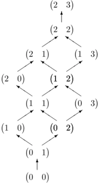
The Hasse diagram for the ordering of vectors in complete games with the given hierarchy

e

n= (2,3) is shown in Figure 1.

2.3

A parameterization theorem for complete games

Carreras and Freixas have given a full parameterization of complete games, up to isomor-phisms, in [4] using vectors as models of coalitions and the partial order≽. We denote the (decreasing) lexicographic order by m, i.e., we have (a1, . . . , an)m(b1, . . . , bn) if there is an

index 1 ≤ h ≤ n with ai = bi for all 1 ≤ i < h and ah > bh. An example is given by

(1,2,1)m(1,1,3).

( 0 0) ( 0 1) ( 1 0) (0 2) ( 1 1) ( 2 0) (1 2) ( 2 1) ( 2 2) ( 2 3) ( 1 2) ( 0 2) ( 0 3) ( 1 3) 6 Q Q k 3 3 3 3 3 QkQ Q Q k Q Q k Q Q k 3 3 QkQ 6

Figure 1: The Hasse diagram for the ordering≽of vectors onne= (2,3).

Theorem 2.2

(a) Assume that a vector en= (n1, n2, . . . , nt)with natural coefficients and a matrix

M=      m1,1 m1,2 . . . m1,t m2,1 m2,2 . . . m2,t .. . ... . .. ... mr,1 mr,2 . . . mr,t     =      e m1 e m2 .. . e mr     

with natural or null coefficients are given, satisfying the following properties: (i) m1,1>0and0≤mi,j≤nj,mi,j∈N0 for1≤i≤rand1≤j≤t,

(ii) mei ◃▹mej for all1≤i < j≤r,

(iii) for each1≤j < tthere is at least one row-index isuch that mi,j>0,mi,j+1 <

nj+1, and

(iv) meimmei+1 for1≤i < r.

Then, there exists a unique complete game (N,W) with invariants (n,e M), i.e., with

e

n as a vector of the cardinalities of the equivalence classes and matrixMwhere their rows consist of the shift-minimal winning vectors.

(b) Two complete games (N1,W1) and (N2,W2) are isomorphic if and only if en1 = en2

As a consequence of this theorem, any complete game can be denoted as (en,M), the pair ofcharacteristic invariants of the game.

In such a vector/matrix representation (characteristic invariants) of a complete game the number of playersnis determined by n=

t

∑

i=1

ni. Although Theorem 2.2 looks technical at

first glance, the necessity of the required properties is easily explained. Obviously, nj ≥1

and 0≤mi,j ≤nj must hold for 1≤i≤r, 1≤j≤t. Ifmei≼mej ormei≽mej then we have

e

mi=mej or eithermeiormej cannot be a shift-minimal winning vector. If for a column-index

1≤j < twe havemi,j= 0 ormi,j+1=nj+1for all 1≤i≤r, then we can check whether we

haveg≈hfor allg∈Nj,h∈Nj+1, which is a contradiction to the definition of the classes

Nj and therefore also for the numbers nj. Obviously a complete game does not change if

two rows of the matrixMare interchanged. Thus we require a given ordering of the rows to avoid repetitions: mstands for the lexicographic ordering of vectors inN0t.

As the desirability relation is total in complete games, it defines for these games a weak ordering on the set of players. For example, writing that a five-player complete game has hierarchy 1 > 2 = 3 = 4 > 5 means that there is one player which has the maximum influence, another one that has the minimum influence and the other three have all the same intermediate influence, in that case we can represent the previous ordering as the vector (1,3,1). We say that two complete games have the same hierarchy if the ordering that defines the desirability relation on them is the same. Thus, if (ne1,M1) and (en2,M2)

are the characteristic invariants of two complete games, they have the same hierarchy if

e

n1=en2.

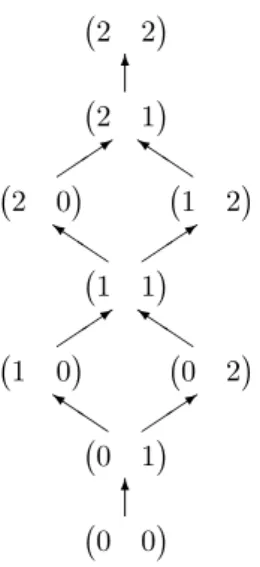
The Hasse diagram for the ordering ≽ of vectors in complete games with the given hierarchyne= (2,2) is shown in next Figure 2.

( 0 0) ( 0 1) ( 1 0) (0 2) ( 1 1) ( 2 0) (1 2) ( 2 1) ( 2 2) 6 Q Q k 3 3 QkQ Q Q k 3 3 QkQ 6

We would like to remark that for t = 1 onlyr = 1 is possible and the requirements in Theorem 2.2 reduce to 1≤m1,1≤n1=n. Also fort= 2 one can easily give a more compact

formulation for the requirements in Theorem 2.2. A complete description of the possible valuesn1, n2, m1,1, m1,2 corresponding to a complete game with parameters n, t = 2, and

r= 1 is given by

1≤n1≤n−1,

n1+n2=n,

1≤m1,1≤n1,

0≤m1,2≤n2−1.

Two important real-world examples of voting weighted games with only one shift-minimal winning vector are (see chapter 8 in [43] for more details on these two examples): the United Nations Security Council –without taking abstention into consideration– and the procedure to amend the Canadian Constitution. These examples have (en,M) = ((5,10),(5,4)) and (en,M) = ((2,8),(1,6)) as respective characteristic invariants.

2.4

Known enumerations for weighted games and for complete games

Let wg(n, t, r) be the number of weighted games with n players, t equivalence classes

N1, . . . , Ntandrshift-minimal winning vectors. Letwg(n,∗, r)3be the number of weighted

games with n players and r shift-minimal winning vectors (independently of the number of equivalence classes, t). Letwg(n, t,∗) be the number of weighted games with nplayers, andtequivalence classesN1, . . . , Nt(independently of the number of shift-minimal winning

vectors, r). We identify wg(n,∗,∗), i.e., the number of weighted games withn players in-dependently of the values of r and t, with simply wg(n). Analogous notations cg(n, t, r),

cg(n,∗, r), cg(n, t,∗) and cg(n) will be used for the respective enumerations of complete games.

The first exact counting can at least be traced back to May [31] which establishes the number of symmetric or anonymous simple games. Any such game withnplayers admits a weighted representation [q; 1,1, . . . ,1

| {z }

n

] where q∈ {1, . . . , n}.

Letwgsym(n),cgsym(n) andsgsym(n) be respectively the number of symmetric: weighted games, complete games and, simple games withnplayers.

Theorem 2.3 wg(n,1,1) =cg(n,1,1) =n=wgsym_{(n) =cg}sym_{(n) =sg}sym_(n)

The number of complete games with one shift-minimal winning vector was determined in [17], and a more refined result appears in [18] (parts 1 and 2 of the next result respectively).

Theorem 2.4 1. cg(n,∗,1) = 2n_−1,

3_{More precisely, the notationwg(n,∗, r) stands for} ∑n t=1

2. cg(n, t,1) =            n, ift= 1 (n+1 2t−1 ) , if2≤t≤ n₂+ 1 0, otherwise

Other formulas have been obtained quite recently. In [16] we can find the next enu-meration, whereF(n) are the Fibonacci numbers, which constitute a well–known sequence of integer numbers defined by the following recurrence relation: F(0) = 0, F(1) = 1, and

F(n) =F(n−1) +F(n−2) for alln >1.

Theorem 2.5 cg(n,2,∗) =F(n+ 6)−(n2_{+ 4n+ 8).}

Let us finally remark that a formula forcg(n,∗,2) is found in [27].

Theorem 2.6 cg(n,∗,2) = n ∑ t=1 cg(n,t,2) = 2·(4n+2n)· ( 6·8n−4n 2₋₃ n(n−3) ( 2n−5 n−4 ) + 2n 2_+3n−2 (n+1)(n−2) ( 2n−3 n−3 )) .

In [27] it is proved that cg(n, t, r) is a quasi-polynomial in n, if t and r are given, and can therefore be automatically computed (without escaping of the problem of capacity limitations). The main purpose of Section 3 is to determinewg(n,∗,1) as well as to obtain other related finer results.

2.5

Power indices

Informally a power index is a numerical measure that estimates the a priori capacity or influence of each player in a simple game. Of course the notion of power is complex and has been analyzed in depth by several authors. An interesting reference is the book by Morriss [32], which analyzes power from a philosophical point of view.

Two prominent power indices are more recognized and used than others, and both known power indices, and both of them are based on the notion of a swing. A coalitionSis aswing fori∈S if and only ifS∈ W but S\ {i}∈ W/ . Letci(N,W) denote the number of swings

of playeriin game (N,W). Then the relative Banzhaf index [2] is defined as

Bzi(N,W) =

ci(N,W)

∑

j∈N

cj(N,W)

while theabsolute Banzhaf index [35] is defined as

Bzi′(N,W) =

ci(N,W)

2n−1 .

TheShapley-Shubik index [38], which is the restriction of the well-known Shapley value [37] for cooperative games, can be expressed as a function of the swings as follows. Letsbe the

cardinality of the swingS foriandcs

i(N,W) be the number of swings forifor coalitionsS

of cardinalitys. Then, SSi(N,W) = n ∑ s=1 (s−1)!(n−s)! n! c s i(N,W).

This less usual formulation of the Shapley-Shubik index will be helpful here for our purposes. The Shapley-Shubik index of a player can be viewed as his/her expected part of a fixed total prize, i.e., the power of a player is meant to be the player’s expected payoff. Dubey and Shapley [9] proved the following result.

Proposition 2.7 If (N,W) is any simple game then, for alli∈N, we have (a) SSi(N,W) =SSi(N,W∗).

(b) Bzi(N,W) =Bzi(N,W∗)andBz′i(N,W) =Bz′i(N,W∗).

The fact that cs_i(N,W) = cs_i(N,W∗) for all s = 1,2, . . . , n justifies (a) and implies that

ci(N,W) =ci(N,W∗), which justifies (b), a property discovered by Dubey and Shapley [9].

3

Counting weighted games with minimum

If we consider a subgame of a weighted game when this game is stripped of its null and veto players, then the original game is weighted if and only if the subgame is weighted and, similarly, the original game is complete if and only if the subgame is complete, see e.g., [44].

Let (en,M) be a complete game witht equivalence classes. By (n,e M)↓we denote

  (ns, . . . , ne ) ,    m1,s . . . m1,e .. . . .. ... mr,s . . . mr,e      ,

where s= 1 if there are no veto players, s= 2 if there are veto players (which would form the strongest class),e=tif there are no null players, ande=t−1 if there are null players (which would form the weakest class). If all players of (n,e M) have veto or are null players (en,M)↓ isempty.

For instance, (n,e M)↓does not change for the system to amend the Canadian Constitu-tion, i.e., (n,e M)↓= (en,M) = ((2,8),(1 6)), whereas (en,M)↓ reduces to ((10),(4)) for the United Nations Security Council, because the five permanent members have veto right.

Lemma 3.1 Let wgc(n, t, r)be the number of non-trivial weighted games witht equivalence classesN1, . . . , Ntand rshift-minimal winning vectors. For r >1 ort >2 we have

wg(n, t, r) =wgc(n, t, r) +

n_∑−1

h=1

2·wgc(n−h, t−1, r) + (h−1)·wgc(n−h, t−2, r), (1) where we define wgc(n, t, r) = 0 for the non-feasible cases n < t or t <1. For r = 1 and

t= 1an additional 1has to be added to the right hand side of Equation (1), and for r= 1 andt= 2an additional termn−1 has to be added to the right hand side of Equation (1).

Proof. Every weighted game arises from a non-trivial weighted game or an empty game

by appendingh1≥0 veto players andh2≥0 null players.

For r= 1 and arbitraryt the set of maximal losing vectors of complete games without null players, i.e., withm1,t≥1, was analytically given in [18] (see next lemma). As forr= 1

the first indices in vectorme1 do not carry any information we omit them.

Lemma 3.2 For a complete game

((

n1, . . . , nt

)

,(m1. . . mt

))

without null players, i.e., with mt ≥1, the complete set of shift-maximal losing vectors is given in the following matrix:

         a1,1 n2 n3 . . . nt a2,1 a2,2 n3 . . . nt a3,1 a3,2 a3,3 . . . nt .. . ... ... . .. ... at−1,1 at−1,2 at−1,3 . . . nt at,1 at,2 at,3 . . . at,t          =:    ea1 .. . e at   , where ai,j:= max { 0,min { nj, −1 + i ∑ h=1 mh− j₋1 ∑ h=1 nh }} for1≤j ≤i≤t.

Note that each vectoreai for 1≤i≤trepresents shift-maximal losing coalitions. Indeed,

these coalitions contain∑i_j=1mj−1 strongest players (according to the desirability relation)

and additionally they also contain the ∑t_j=i+1nj weakest players, i.e., those players that

belong to thet−i weakest equivalence classes, from thei+ 1th class to the tth last class. If in one of these coalitions an additional player was added or a weaker player was replaced by a stronger one, then the new vectoreb representing the coalition would contain at least

∑i

j=1mj players for each 1≤i≤t and therefore would be winning.

The conditions (i)–(iv) of Theorem 2.2-(a) reduce to 1≤m1≤n1, 0≤mt≤nt−1, and

1≤mh≤nh−1 for allhsuch that 2≤h≤t−1. We remark that if a complete game with

r= 1 has null players, then the complete set of shift-maximal losing vectors is given by the vectors in Lemma 3.2 except for the last vectoreat. We would like to remark too that eatis

a losing vector which is not maximal and that there is a typo in the remark of [18], i.e., the first row (instead of the last one) must be deleted.

Having an analytic description of the shift-maximal losing vectors at hand it is not too hard to characterize the set of weighted games analytically. Indeed, already in [11] the non-trivial weighted games withr= 1, i.e., those having exactly one shift-minimal winning vector, were completely classified.

Theorem 3.3 A non-trivial complete game (n,e M) with r = 1 is a weighted game if and only if either t= 1 ort= 2andm2∈ {1, n2−1}.

Proof. Due to Theorem 2.2 we can assume t ≥ 2. For t = 2 the shift-maximal losing

vectors are given by

(m1−1, n2) and (m1+c, m2−1−c),

wherec= min (n1−m1, m2−1). Choosing w1= 1 we conclude

m1+w2m2 > m1−1 +w2n2,

m1+w2m2 > m1+c+w2(m2−1−c),

which is equivalent to w2 < _n2−1_m

2 and (1 +c)w2 > c. If m2 =n2−1 or c= 0, which is equivalent to m2 = 1, there exists a solution for w2. If m2 ≤ n2−2 and c ≥ 1 the two

inequalities are contradicting.

Now we consider the remaining cases t≥3. Here the vectors

(m1−1, n2, . . . , nt), and (m1+ 1, m2−1, m3−1, n4, . . . , nt)

are losing vectors (the second not necessarily shift-maximal). Thus forw1= 1 we have

m1+ t ∑ j=2 wjmj > m1−1 + t ∑ j=2 wjnj, m1+ t ∑ j=2 wjmj > m1+ 1 +w2(m2−1) +w3(m3−1) + t ∑ j=4 wjnj,

from which we conclude 1> w2+w3 andw2+w3>1, which is a contradiction.

Thus together with Lemma 3.1 and Theorem 2.3 we can conclude:

Theorem 3.4 Forn≥1 we have

f wg(n,1,1) = n−1, f wg(n,2,1) = { 0 if n≤2, n2_{−6n+ 9 if n≥3,} f wg(n, t,1) = 0 if t≥3, wg(n,1,1) = n, wg(n,2,1) = { n−1 if n≤2, 2(n−2)2_{+ 2 if n≥3,} wg(n,3,1) = { 0 ifn≤3, 5n3_−48n2_+157n−174 6 ifn≥4, wg(n,4,1) = { 0 if n≤5, n4−16n3+95n2−248n+240 12 if n≥6, wg(n, t,1) = 0 if t≥5.

Adding up the previous enumerations we get the following compact expression for the total number of weighted games with a unique shift-minimal winning vector.

Corollary 3.5 wg(n,∗,1) =    2n_{−1 ifn≤5} n4_−6n3_{+ 23n}2_{−18n+ 12} 12 ifn≥6

Thus, the numbers of weighted games wg(n,∗,1) and complete games cg(n,∗,1) (see The-orem 2.4) coincide for n≤5 players, but their ratio converges to zero asn increases. An asymptotic upper bound for weighted games is given in [7] and an asymptotic lower bound for complete games is given in [36], where these games are called regular Boolean functions. Many useful and accurate asymptotic estimations for simple games and subclasses of them are provided in [24].

4

Analysis of voting power for bipartite complete games

with minimum

Many papers have been devoted to study classes of games for which two or more power indices provide the same rankings in every game of such classes, see e.g., [8], [5], [13]. However, as far as we know, very little has been studied about comparisons of different games depending on how a given power index acts on them.

In this section we will consider complete games with two types of equivalent players and with only one shift-minimal winning vector. For these games we will give explicit formulas to calculate some efficient power indices. Since the games have only two types of equivalent players and the considered power indices are efficient, it will be possible to totally rank these games according to the behavior of the power index on players that belong to a fixed class. Of course, the order obtained considering the power over a type of players for bipartite complete games with games with minimum is reversed if the power index is evaluated over players that belong to the other equivalence class.

An important tool to this purpose is monotonicity in Young’s sense [45] which was used to give a characterization of the Shapley value that avoids additivity. If we assume a fixed set of playersN we writeWBiW′ whenever ifS is a swing foriin W′ then S is a swing

fori in W. RelationBi allows us to qualitatively compare the position of a given playeri

in two games. However, we do not see a direct application of such a monotonicity for most of the cases we are going to study.

4.1

Allowable rankings for the Shapley-Shubik index

The main purpose of this subsection is to study the allowable hierarchies that the Shapley-Shubik index produces when applied to different bipartite complete (t = 2) games with minimum (r= 1). We also illustrate the difficulty to extend similar results for other power indices.

Proposition 4.1 Let(n,e M)be a complete game withne= (n1, n2)andM= (

a b), where

(1) For a player of type1 the number of coalitions where he is a swing player is given by c1= n2 ∑ i=b+1 ( n1−1 a−1 ) · ( n2 i ) + min{_∑b,n1−a} i=0 ( n1−1 a+i−1 ) · ( n2 b−i ) .

(2) For a player of type2 the number of coalitions where he is a swing player is given by

c2= min{b−_∑1,n1−a} i=0 ( n1 a+i ) · ( n2−1 b−i−1 ) .4

(3) The Shapley-Shubik power indexSS1(a, b, n1, n2) of a player of type1 is given by

1 n! · n2 ∑ i=b+1 (n₁₋1 a−1 ) ·(n2 b ) ·(a+i−1)!·(n−a−i)! + (a+b−1)!·(n−a−b)! n! · min_{b,n_∑1−a_} i=0 (n1−1 a+i−1 ) ·(n2 b−i ) .

(4) The Shapley-Shubik power indexSS2(a, b, n1, n2) of a player of type2 is given by

(a+b−1)!·(n−a−b)! n! · min_{b_−∑1,n₁₋a_} i=0 ( n1 a+i ) · ( n2−1 b−i−1 ) . (5) Forb≥1we have SS2(a, b, n1, n2)−SS2(a, b−1, n1, n2) = (a+b−2)!·(n−a−b)!·n1· (n1−1 a−1 ) ·(n2−1 b−1 ) n! >0. (6) Fora≥2 we have SS2(a−1, b, n1, n2)−SS2(a, b, n1, n2) =    0, ifb= 0 (a+b−2)!·(n−a−b)!·(n2−1)· (_n1 a₋1 ) ·(n2−2 b₋1 ) n! , ifb≥1 Proof.

(1) The vectors representing coalitions where a player of type 1 is a swing player are given by (a, b+ 1), (a, b+ 2),. . ., (a, n2) and (a, b), (a+ 1, b−1), (a+ 2, b−2), . . ., (c, d) where: (c, d) = { (a+b,0), ifa+b≤n1 (n1, a+b−n1), otherwise.

The number of swings for a player of type 1 for an arbitrary vector (x, y) is: (n_x1−₋₁1)·(n2

y

)

. 4_{Unfortunately we cannot apply Vandermonde’s identity} ∑k

j=0 (m j )( n k−j ) =(m+_kn)directly.

(2) The vectors representing coalitions where a player of type 2 is a swing player are given by (a, b), (a+ 1, b−1), (a+ 2, b−2),. . ., (e, f) where: (e, f) = { (a+b−1,1), ifa+b≤n1 (n1, a+b−n1), otherwise.

The number of swings for a player of type 2 for an arbitrary vector (x, y) withy >0 is: (n1 x ) ·(n₂₋1 y−1 ) .

(3)-(4) These results follow from the definition given in this paper for the Shapley-Shubik index and parts (1)-(2) respectively.

(5) Forn1−a≤b−2 we have SS2(a, b, n1, n2)−SS2(a, b−1, n1, n2) = (a+b−2)!(n−a−b)! n! · [_n∑1−a i=0 (n1 a+i )(n₂₋1 b₋i₋1 ) ( a+b−1−(n−a_n−₂₋b+1)(_b+i+1b−i−1) )]

and forn1−a≥b−1 we have:

SS2(a, b, n1, n2)−SS2(a, b−1, n1, n2) = (a+b−2)!(_n!n−a−b)!· [ (a+b−1) b∑−1 i=0 (_n1 a+i )(_n2−1 b₋i₋1 ) −(n−a−b+ 1) b∑−2 i=0 (_n1 a+i )(_n2−1 b₋i₋2 )] ,

both of which can be simplified to the stated expression. (6) Similar to (5).

Corollary 4.2 1. For a given vector(n1, n2)let((m1, m2))and((m′1, m′2))be two

differ-ent complete simple games, i.e., 0< m1, m′1≤n1 and0≤m2, m′2< n2. Ifm1≥m′1

and m2 ≤ m′2 then SS2(m1, m2)≤ SS2(m′1, m′2) and SS1(m1, m2) ≥ SS1(m′1, m′2),

where equality holds if and only if m2=m′2= 0.

2. For a given vector(n1, n2):

1

n < SS1(1, n2−1)≤SS1(m1, m2)≤SS1(n1,1)< SS1(c,0) =

1

n1

(2) where cis any integer number between1 andn1.

Inequalities (2)imply 1

n > SS2(1, n2−1)≥SS2(m1, m2)≥SS2(n1,1)> SS2(c,0) = 0

Remark 4.3 We have implemented a computer program which can determine the Banzhaf and the Shapley-Shubik power index for bipartite complete games with minimum. For the casen1= 3,n2= 7 we have the following ordering with respect toSS1:

(3,0) = (2,0) = (1,0)>(3,1)>(3,2)>(2,1)>(3,3)>

(2,2)>(3,4)>(1,1)>(2,3)>(3,5)>(1,2)>(2,4)>

(3,6)>(1,3)>(2,5)>(1,4)>(2,6)>(1,5)>(1,6)

Note that, in general, for an arbitrary pair (n1, n2) the rankings of some games with

respect toSS1 or Bz1(printed in bold in the previous example) are fixed. We refer to the

games of type (c,0) forc > 0 which are always tied among them and situated on the top of the ranking and, oppositely, the game (1, n2−1) which is always situated at the bottom

of the ranking. These extreme games are highlighted in black in the previous example for

n1 = 3, n2 = 7. Additionally, Corollary 4.2 provides some constraints on the rankings of

the different games with respect toSS1 orBz1:

1. leaving the first component fixed:

(3,1)>(3,2)>(3,3)>(3,4)>(3,5)>(3,6); (2,1)>(2,2)>(2,3)>(2,4)>(2,5)>(2,6); and (1,1)>(1,2)>(1,3)>(1,4)>(1,5)>(1,6).

2. leaving the second component fixed:

(3,1)>(2,1)>(1,1); (3,2)>(2,2)>(1,2); (3,3)>(2,3)>(1,3); (3,4)>(2,4)>(1,4); (3,5)>(2,5)>(1,5) and (3,6)>(2,6)>(1,6).

Taking into account all these restrictions we have that for the given hierarchy n = (3,7) we have 13 weighted games, three of which are of type (c,0) and give the maximum value 1/n1= 1/3 for theSS1to three most powerful players; the ranking of all other games with

respect toSS1 is strict so that there are, in principle, 10! potential strict orderings for the

power of SS1 over the set of these games, but Corollary 4.2 guarantees that at most 12 of

these rankings are possible.

4.2

Comparisons for the two Banzhaf indices

As we shall see in this section, we find for the relative Banzhaf index a similar result to that one obtained for the Shapley-Shubik index (for less than 100 players), while it fails for the absolute Banzhaf index.

The relative Banzhaf power index Bz1(a, b, n1, n2) of a player of type 1 is given by

c1

n1·c1+n2·c2

.

The relative Banzhaf power indexBz2(a, b, n1, n2) of a player of type 2 is given by

c2

n1·c1+n2·c2

The absolute Banzhaf power indexBz₁′(a, b, n1, n2) of a player of type 1 is given by

c1

2n−1.

The absolute Banzhaf power indexBz₂′(a, b, n1, n2) of a player of type 2 is given by

c2

2n−1.

Remark 4.4 For the Banzhaf absolute power index, Corollary 4.2 is wrong, and an example is given byn= 4,n1 =n2= 2 and the games ((2,1)),((1,1))with Banzhaf values

(₃ 8, 1 8 ) , (₄ 8, 2 8 )

, respectively. Another example is given by n = 7, n1 = 3, n2 = 4 and the games

((3,1))and((2,2))with absolute Banzhaf indices (15₆₄,₆₄1),(26₆₄,10₆₄), respectively.

Example 4.5 (Ties) Let us consider the equality case in Corollary 4.2 for the relative Banzhaf power index, i.e., where the powers sum up to 1. Form2=m′2= 0 equality holds.

Other examples are given by

• n= 7,n1= 3, and the games ((3,3)), ((1,2)) with Banzhaf numerators (5,3), (20,12)

• n= 8,n1= 2, and the games ((2,5)), ((1,4)) with Banzhaf numerators (7,5), (42,30)

• n= 9,n1= 6, and the games ((6,2)), ((1,1)) with Banzhaf numerators (4,2), (12,6)

• n = 13, n1 = 5, and the games ((5,7)), ((2,5)) with Banzhaf numerators (9,7),

(1044,812)

• n = 13,n1 = 9, and the games ((6,2)), ((1,1)) with Banzhaf numerators (736,288),

(23,9)

These are all examples where (m1, m2)>(m′1, m′2) or (m1, m2)<(m′1, m′2). If we assume

m1≥m′1 andm2≤m′2then there is no further example forn≤32.

Remark 4.6 For the relative Banzhaf power index Corollary 4.2 is true for alln≤100. This suggests to ask whether Corollary 4.2 is true for the relative Banzhaf index for alln.

Conjecture 4.7 (1) Forb≥1 we have Bz2(a, b, n1, n2)−Bz2(a, b−1, n1, n2)>0.

(2) For a ≥2 we have Bz2(a−1, b, n1, n2)−Bz2(a, b, n1, n2)≥0 which equals zero for

b= 0 and otherwise it is positive.

It would imply a corollary analogous to Corollary 4.2.

Corollary 4.8 1. For a given vector(n1, n2)let((m1, m2))and((m′1, m′2))be two

differ-ent complete simple games, i.e., 0< m1, m′1≤n1 and0≤m2, m′2< n2. Ifm1≥m′1

and m2 ≤m′2 then Bz2(m1, m2) ≤Bz2(m′1, m′2) and Bz1(m1, m2) ≥ Bz1(m′1, m′2),

2. For a given vector(n1, n2): 1 n < Bz1(1, n2−1)≤Bz1(m1, m2)≤Bz1(n1,1)< Bz1(c,0) = 1 n1 (3) where cis any integer number between1 andn1.

Inequalities (3)imply 1

n> Bz2(1, n2−1)≥Bz2(m1, m2)≥Bz2(n1,1)> Bz2(c,0) = 0

where cis any integer number between1 andn1.

However, the ranking over different games for Shapley-Shubik and relative Banzhaf index are not necessarily the same, as the following example illustrates.

Example 4.9 For the case n1 = 3, n2 = 7 we have checked the following rankings with

respect to Bz1:

(3,0) = (2,0) = (1,0)>(3,1)>(2,1)>(1,1)>(3,2)>

(2,2)>(3,3)>(1,2)>(2,3)>(3,4)>(1,3)>(2,4)>

(3,5)>(2,5)>(1,4)>(3,6)>(2,6)>(1,5)>(1,6)

This ranking of different games with vector en= (3,7) does not coincide with the ranking obtained for theSS1but, restricted to weighted games, it is one of the 12 expected rankings

for theSS1 according to Corollary 4.2.

Remark 4.10 One might conjecture that Corollary 4.2 holds for some effective generalized power indices as for example semivalues. Semivalues for simple games (or power semi-indices) are uniquely determined as those power indices that satisfy: symmetry, positivity, dummy player property and transfer (see [6]) and with specific coefficients{pj}nj=1 such that ∑n

j=1pj

(_n−1

j−1 )

= 1 and pj ≥ 0 for all j. The absolute Banzhaf power index is given by

pj= 1/2n−1 for all1≤j≤nand the Shapley-Shubik power index is given bypj=

1

n(n_j−−₁1).

The (unnormalized) power, SV, of playeri is given by

SV(i) := n ∑ i=1 p_|S|·csi. where|S|=s.

Let us consider the following example: n = 10, n1 = 7, and the games ((7,1)) and

((1,2)) with power index numerators (3p7+ 3p8+p9, p7), (36p2+p3,35p2). This example

is a counterexample to Corollary 4.8 if and only if

207p2p7+ 315p2p8+ 105p2p9−3p3p7<0.

If we assumepj=pn−j−1 then this is equivalent to

p2·(105p0+ 325p1+ 207p2−3p3)<0,

5

Results preserved by duality

This section establishes a simple but significant result on enumerations and highlights that the results obtained in the previous section about power indices are preserved by duality.

Let us recall that the dual game of (N,W) is (N,W∗) where: W∗={S⊆N : N\S /∈

W}. Then it is not difficult to check the following:

Lemma 5.1 (i) (N,W)is weighted if and only if(N,W∗)is weighted, and if[q;w1, . . . , wn] is an integer representation for (N,W)then[T −q+ 1;w1, . . . , wn]is an integer rep-resentation for (N,W∗)whereT =

n

∑

i=1

wi and vice versa.

(ii) i % j if and only if i %∗ j where %∗ stands for the desirability relation for game (N,W∗). Thus, (N,W) is complete if and only if (N,W∗) is complete, and the ≈ -classes Ni for (N,W) and its orderingN1 > N2· · · > Nt are preserved by %∗, i.e.,

(N,W)and(N,W∗)have the same rankingne.

(iii) The complete game(N,W)has the vector en= (n1, . . . , nt)∈Nt>0 and the matrix

M=      m1,1 m1,2 . . . m1,t m2,1 m2,2 . . . m2,t .. . ... . .. ... mr,1 mr,2 . . . mr,t     =      e m1 e m2 .. . e mr     

as characteristic invariants (hence, fulfilling properties (1)-(4) in Theorem 2.2) and matrix L=      l1,1 l1,2 . . . l1,t l2,1 l2,2 . . . l2,t .. . ... . .. ... ls,1 ls,2 . . . ls,t     =       el1 el2 .. . els      

of shift-maximal losing vectors if and only if the complete game (N,W∗) has vector

e n= (n1, . . . , nt)∈Nt>0 and matrix M∗₌      n1−ls,1 n2−ls,2 . . . nt−ls,t n1−ls−1,1 n2−ls−1,2 . . . nt−ls−1,t .. . ... . .. ... n1−l1,1 n2−l1,2 . . . nt−l1,t     =       f m∗₁ f m∗₂ .. . f m∗_s      

as characteristic invariants (hence, fulfilling properties (1)-(4) in Theorem 2.2-(a)) and matrix L∗₌      n1−mr,1 n2−mr,2 . . . nt−mr,t n1−mr−1,1 n2−mr−1,2 . . . nt−mr−1,t .. . ... . .. ... n1−m1,1 n2−m1,2 . . . nt−m1,t     =       e l₁∗ e l₂∗ .. . e l_r∗      

Let cg(n, t, r) be the number of complete games with n players, with t equivalence classes and r shift-maximal losing vectors and similar notation for: cg(n,∗, r), wg(n, t, r) and wg(n,∗, r). Lemma 5.1 allows us to deduce the next corollary and describes how the bijection for characteristic invariants works.

Corollary 5.2 cg(n, t, r) =cg(n, t, r)andwg(n, t, r) =wg(n, t, r).

The application of this Corollary and the results on enumerations in Sections 2 and 3 to games with one shift-maximal losing vector gives the enumerations for complete games and for weighted games respectively. An analogous version of Theorem 2.4 is given by

Corollary 5.3 1. cg(n,∗,1) = 2n_−1, 2. cg(n, t,1) =            n, ift= 1 (_n+1 2t₋1 ) , if2≤t≤ n₂+ 1 0, otherwise and an analogous version of Corollary 3.5 is given by

Corollary 5.4 wg(n,∗,1) =    2n−1, ifn≤5 n4−6n3+ 23n2−18n+ 12 12 , ifn≥6

Due to Proposition 2.7 and Lemma 5.1 it follows that the results in Section 4 for the Shapley-Shubik index extend to complete games with one-shift maximal losing vector, since for any given (n1, n2) andM= (a b), the dual game is given by the same vector and matrix

L∗_{= (n1−a n2−b) which corresponds to matrix M}∗_where: (i) M∗= (n1−a+ 1 0) ifb= 0, otherwise: (ii) M∗= ( n1−a+ 1 0 n1−a−b+ 1 n2 ) ifa+b−1≤n1, (iii) M∗= ( n1−a+ 1 0 0 n−a−b+ 1 ) ifa+b−1> n1.

Thus Proposition 4.1 has a simple analogue, and therefore Corollary 4.2 has a simple ana-logue too. The conjecture stated for the relative Banzhaf index derived for the computation up to 100 players is also open in this dual context.

6

Future work

Any progress concerning enumeration of games, likecg(n, t, r) orwg(n, t, r), will be a signif-icant advance in both directions: either providing new formulas or providing tighter bounds. In [27] it is proved thatcg(n, t, r) is a quasi-polynomial in n, if tand rare given, and can therefore be automatically computed (without escaping of the problem of capacity limita-tions). We wonder whether these automatic computations can be performed for the number

wg(n, t, r) of weighted games.

We also encourage research in other classes of simple games. For instance, roughly weighted games (considered in [44] and extensively studied in [20]) which are complete, i.e., roughly weighted complete games with n players and t types of equivalent players to determinercg(n, t, r).

As a future research concerning section 4 (and 5) it would be nice to find the proofs of our conjectures 4.7 and 4.8. It seems likely that these conjectures are true since they hold for games with less than 100 players. It would also be of interest to know whether the Shapley-Shubik power index is the unique semiindex (semivalue restricted to simple games) that satisfies Corollary 4.2.

Acknowledgments

The authors are grateful to the two referees of this paper for their interesting comments and also for their exhaustive reports that contributed to improve the original submitted version.

References

[1] J.M. Alonso–Meijide and C. Bowles,Generating functions for coalitional power indices: an application to the IMF, Annals of Operations Research137(2005), 21–44.

[2] J.F. Banzhaf, Weighted voting doesn’t work: A mathematical analysis, Rutgers Law Review19(1965), 317–343.

[3] E.F. Brickell,Some ideal secret sharing schemes, J. Combin. Math and Combin. Com-put.9(1989), 105–113.

[4] F. Carreras and J. Freixas, Complete simple games, Mathematical Social Sciences 32

(1996), 139–155.

[5] , On ordinal equivalence of power measures given by regular semivalues, Math-ematical Social Sciences55 (2008), 221–234.

[6] F. Carreras, J. Freixas, and M.A. Puente,Semivalues as power indices, European Jour-nal of OperatioJour-nal Research149(2003), 676–687.

[7] B. Keijzer de, T. Klos, and Y. Zhang,Enumeration and exact design of weighted voting games, Proceedings of the 9th International Conference on Autonomous Agents and Multiagent Systems, vol. 1, 2010, pp. 391–398.