Development of a time-resolved quantitative surface-temperature measurement technique and its application in short-duration wind tunnel testing

(1)

APPLICATION IN SHORT-DURATION WIND TUNNEL TESTING

DISSERTATION

zur Erlangung des mathematisch-naturwissenschaftlichen Doktorgrades „Doctor rerum naturalium“

der Georg-August-Universität Göttingen

im Promotionsprogramm ProPhys

der Georg-August University School of Science (GAUSS)

vorgelegt von

S

TEFFEN

R

ISIUS aus Emden

(2)

Prof. Dr. Andreas Dillmann,

Georg-August-Universität Göttingen, Institut für Nichtlineare Dynamik und Deutsches Zentrum für Luft- und Raumfahrt e.V., Institut für Aerodynamik und Strömungstechnik

Prof. Dr. Martin Rein,

Dr. Stefan Hein,

Deutsches Zentrum für Luft- und Raumfahrt e.V., Institut für Aerodynamik und Strömungstechnik, Abteilung Hochgeschwindigkeitskonfiguration (AS-HGK)

Dr. Christian Klein,

Deutsches Zentrum für Luft- und Raumfahrt e.V., Institut für Aerodynamik und Strömungstechnik, Abteilung Experimentelle Verfahren (AS-EXV)

Mitglieder der Prüfungskommission Referent:Prof. Dr. Andreas Dillmann,

Korreferent:Prof. Dr. Martin Rein,

Weitere Mitglieder der Prüfungskommission Prof. Dr. Wolfgang Glatzel,

Georg-August-Universität Göttingen, Institut für Astrophysik Prof. Dr. Stephan Herminghaus,

Georg-August-Universität Göttingen, Institut für Nichtllineare Dynamik und Max-Planck-Institut für Dynamik und Selbstorganisation

Prof. Dr. Wolfram Kollatschny,

Georg-August-Universität Göttingen, Institut für Astrophysik Prof. Dr. Andreas Tilgner,

Georg-August-Universität Göttingen, Institut für Geophysik

(3)

The dissertation was an outcome of my research at the German Aerospace Center (DLR) in Göttingen. Without the support and advice of many people this work would have never been possible. First of all I would like to acknowledge my academic supervisor Prof. A. Dillmann and academic co-supervisors Prof. M. Rein, Dr. S. Hein and especially Dr. C. Klein for the continuous advice and support of this dissertation.

I am also very thankful to all (former) members of the Pressure- and Temperature-Sensitive Paint group in the Experimental Methods department of DLR, in particular Dr. W. Beck, Dr. M. Costantini, B. Dimond, S. Dufhaus, Prof. Y. Egami (Aichi Inst. of Techn.), Dr. R. Engler, Dr. U. Fey, Dr. U. Henne, Dr. M. Hilfer, Dr. C. Klein, W. Lang, J. Lemarechal, Prof. M. Munekata (Kumamoto University), Dr. W. Sachs, A. Weiss and Dr. D. Yorita. I am very glad and thankful to be part of this group of wonderful people, who have become far more than colleagues to me.

The wind tunnel measurement campaigns would not have been possible without the help of the colleagues M. Aschoff, Dr. M. Bruse, A. Grimme, S. Hucke, R. Kahle, M. Löhr and K. Plettenberg from the German-Dutch Wind Tunnels (DNW). I am also grateful to the Head of the Experimental Methods department, Dr. L. Koop, and many other colleagues from DLR Göttingen who supported me throughout the years, in particular J. Agocs, Dr. T. Ahlefeldt, U. Becker, C. Fuchs, Dr. S. Haxter, T. Kleindienst, Dr. S. Koch, Dr. D. Schmeling, Dr. J. Martinez Schramm, I. Micknaus, Dr. H. Rosemann, C. Rosenstock, Dr. A. Schröder and Dr. A. Wagner. For the completion of this thesis it was indispensable what I have learned from my former colleagues and advisers, in particular Prof. E. Bodenschatz, Dr. F. Di Lorenzo, Dr. S. Klein, S. Lambertz and especially Prof. H. Xu (Tsinghua University) at the Max-Planck-Institute for Dynamics and Self-Organization as well as Prof. K. Asai and Prof. H. Nagai from Tohoku University.

The good cooperation with external partners, in particular Prof. U. Beifuß and Dr. V. Ondrus (University of Hohenheim); P. Dür and G. Holst (PCO AG); Dr. P. Guntermann, A.-K. Hensch and J. Quest (ETW GmbH); S. von Deetzen and M. Müller (Deharde GmbH); Dr. S. Schaber, Dr. G. Schrauf and A. Styles (Airbus) is also acknowledged.

Last but not least I want to thank my family and friends, in particular C. Alberts, M. Boyraz, H. Buhr, Cocu family, Dr. A.&M. Eberle, P. Federmann, Folkers family, Goldbach family, Hallenga family, K. Hank, J. Hinze, A. Jakobi, R. Kaufmann, D. Kreutzburg, M. Lüther, Moots family, Müller family, Przysucha family, S. Randahl, Rauch family, Reimold family, Risius family, K. Roskam, Sabat family, M. Schmidt, Dr. O. Schütte, Dr. I. Stroescu, Tielker family, Wiedermann family and Wild family but most of all my parents and my daughter for everything.

(4)

(5)

(6)

In this cumulative thesis, a time-resolved quantitative temperature-sensitive paint (TSP) measure-ment technique was developed and used to measure temperatures at subsonic and up to hypersonic flow velocities in two different short duration wind tunnels. Based on this measurement technique it was possible to calculate the heat transfer into a wedge model in the High Enthalpy Shock Tunnel Göttingen (HEG). Furthermore, the measurement technique was developed further to determine the location of laminar-turbulent transition on the two-dimensional wind tunnel modelPaLASTra, which offers a quasi-uniform streamwise pressure gradient, in the Cryogenic Ludwieg-Tube Göt-tingen (DNW-KRG) with temporal and spatial accuracy that had not been reached before. The quantitative temperature results obtained from TSP measurements allowed the systematic analysis of unit Reynolds number, Mach number and pressure gradient effects on laminar-turbulent transition at flow speeds fromM=0.35 to 0.77. The following is a list of the main findings:

1. The usability of TSP to measure temperatures on a wedge surface in a hypersonic, short-duration flow was demonstrated. The time-resolved temperature information was used to calculate heat load, making use of those assumptions generally applied to these types of flows. Both temperature and heat load results on the surface of a ramp model placed in a Mach 7.4 HEG flow are shown. A Medtherm coaxial thermocouple situated at one position on the model was used to calibrate the TSP (viz. to obtain the thermal parameterρckfor the TSP). An average heat load in the interrogation region of 0.73±0.07 MWm−2was found. Furthermore, a detailed discussion of error sources and uncertainties was carried out.

2. The correction of temperature effects on the determined transition Reynolds numbers and critical

N-factors in the Cryogenic Ludwieg-Tube Göttingen. The temperature difference between the flow and model surface which is required for TSP transition measurements influences boundary-layer instability and the measured transition locations. It was corrected by a linearized fit which relates the adiabatic and non-adiabatic transition Reynolds numbers to the wall temperature ratios. This correction was made possible by the development of a time-resolved and quantitative surface temperature measurement with TSP. The temperature distributions measured by TSP were also used as input for boundary-layer calculations and linear stability analysis which led to a correction of temperature influences on criticalN-factors.

3. It was shown that modifications of thePaLASTramodel proved to be useful in order to reduce the magnitude of pressure fluctuations, caused by flow separation at the trailing edge of the original model, below the minimum measurable quantity. The separation-induced pressure fluctuations and their influence on the location of laminar-turbulent transition was investigated in DNW-KRG. As a result, an additional aft part was installed at the trailing edge of thePaLASTramodel and used for the further investigations.

4. It was found that thePaLASTramodel exhibits a quasi-uniform streamwise pressure gradient, characterized by the incompressible shape factor, H12, or the Hartree parameter,βH. A linear

(7)

approximations were an important step to obtain the further results which are described below. 5. The unit Reynolds number effect on the transition Reynolds number was explained and quantified by the relation between the spectral level and the frequency leading to Tollmien-Schlichting (T-S) induced transition. To this end, a power law between unit Reynolds number,Re1, and transition

Reynolds number,Retr, was used, withRetr∼Reα₁III. The exponentαIIIwas found to range between

0.1 and 0.6 for accelerated flows, which agrees well with earlier measurements in hypersonic wind tunnels.

6. The first quantitative description of the Mach number effect (or ‘compressibility effect’) in a subsonic flow. This quantification was made possible by using the unique feature of DNW-KRG to be able to vary Mach number, unit Reynolds number and total temperature separately. Therefore, the systematic variation of M, Re1 andH12 was combined with a detailed analysis of the free

stream turbulence spectrum in the wind tunnel. Furthermore, it was shown that not the RMS turbulence level alone is of importance for T-S induced transition, but the spectral level in the relevant frequency range has to be considered as well.

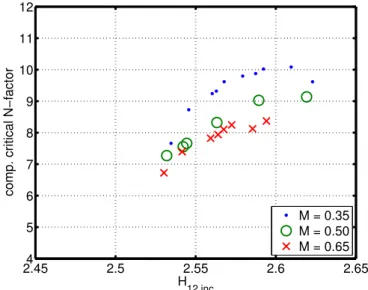
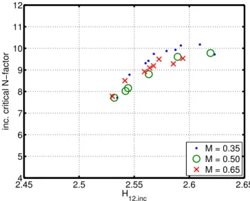
7. The finding of the criticalN-factor ofNcomp≈9.0, for compressible linear stability calculations, andNinc≈9.5 for incompressible calculations for the modifiedPaLASTramodel in DNW-KRG. It was shown that the exclusive incorporation of compressibility into linear stability analysis leads to a larger deviation in the determined critical N-factors (maximal variation of all data points:

∆Ncomp=4.90), as compared to the criticalN-factors calculated by incompressible linear stability analysis (∆Ninc=4.29).

8. A correction method was proposed that takes into account the varying influence of the spectral level of total pressure fluctuations (p?) on the initial T-S wave amplitude. By this correction the standard deviations and maximal variations of the critical N-factors were reduced and led to compressible criticalN-factors (∆Ncomp,p? =4.02) which are similar to or smaller than in the

incompressible case (∆Ninc,p? =4.06).

9. It was found that the determined critical N-factors show a dependency onH₁₂ which is in agreement with earlier findings. It is plausible that this effect is related to the receptivity process, which can be reduced by incorporating the receptivity dependency of acoustic disturbances (C) on incidence angles. A correction method was developed which reduces the dependency onH12

and leads to even smaller maximal variations of the critical N-factors of∆Ninc,p?_,_C =3.81 and ∆Ncomp,p?_,_C=3.53.

10. It was found that the correlated critical N-factors are dependent on Mach number. The dependency is larger for the compressible than for the incompressibleN-factors, with a variation of the mean ofδNcomp≈1.7 andδNinc≈0.6, respectively. The Mach number dependency was further reduced by the correction methods described above.

(8)

(9)

Abstract vi Nomenclature xiii I PREAMBLE 1 1 Motivation 3 2 Introduction 5 2.1 Historical introduction . . . 5

2.2 Relevance for today’s world . . . 6

2.3 Outline and major achievements of the thesis . . . 7

2.4 Impact of the work and other achievements . . . 8

II ANALYSIS AND RESULTS 11 3 Determination of heat transfer in a hypersonic flow (Risius et al., 2017) 13 3.1 Abstract . . . 13

3.2 Introduction . . . 14

3.3 Experimental section . . . 16

3.4 Temperature determination using TSP . . . 17

3.5 Determination of heat loads . . . 19

3.5.1 Temperature sensors . . . 19

3.5.2 Evaluation of heat transfer from Medtherms and TSP . . . 19

3.6 Results and discussion . . . 20

3.6.1 HEG results; TSP images (raw data) . . . 20

3.6.2 TSP temperature results . . . 23

3.6.3 TSP heat load results . . . 24

3.6.4 Accuracy of TSP temperature and heat load results . . . 26

3.6.4.1 Thermal parameterρck: material properties . . . 26

3.6.4.2 The interrogation area . . . 28

3.6.4.3 Correction for time response of the paint . . . 29

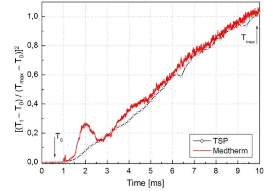
3.6.4.4 Normalized TSP and Medtherm temperatures . . . 33

(10)

4 Mach number effects in the Cryogenic Ludwieg-Tube Göttingen (Risius et al.,

2018a) 35

4.1 Abstract . . . 36

4.3 Experimental Setup and Test Conditions . . . 37

4.4 Results . . . 41

4.4.1 Mach number influence on the transition Reynolds number . . . 41

4.4.2 Compressible and incompressibleN-factor analysis . . . 43

4.5 Conclusions . . . 44

5 Unit Reynolds number, Mach number and pressure gradient effects on laminar-turbulent transition in two-dimensional boundary layers (Risius et al., 2018b) 47 5.1 Abstract . . . 48

5.2.1 Unit Reynolds number effect . . . 49

5.2.2 Mach number effect . . . 49

5.2.3 Transition prediction by theeN-method and correction of determined criti-calN-factors . . . 50

5.2.4 Compressible and incompressibleN-factor analysis . . . 51

5.2.5 Scope of the work . . . 51

5.2.5.1 Unit Reynolds number effect . . . 51

5.2.5.2 Mach number effect . . . 52

5.2.5.3 Correction of compressible and incompressible criticalN-factors 52 5.2.6 Outline of the paper . . . 52

5.3 Experimental setup and boundary layer computations . . . 53

5.3.1 The Cryogenic Ludwieg-Tube Göttingen . . . 53

5.3.2 The two-dimensional wind tunnel modelPaLASTra . . . 53

5.3.3 Boundary layer computations . . . 55

5.3.4 Linear stability analysis . . . 57

5.4 Analysis of stability modifiers . . . 58

5.4.1 Spectral analysis of total pressure fluctuations . . . 59

5.4.2 Correction of non-adiabatic surface temperature . . . 60

5.4.3 Influence of shape factor on transition Reynolds number . . . 62

5.4.4 Influence of unit Reynolds number (Re?₁) on transition Reynolds number (Re?_tr) . . . 63

5.4.5 Relation between frequency of most amplified T-S wave at the transition location (ftr) and the unit Reynolds number (Re?₁) . . . 65

5.4.6 Combination of equations . . . 67

5.4.6.1 Relationship between the unit Reynolds number (Re?₁) and the spectral level of total pressure fluctuations (p?) . . . 68

(11)

5.4.6.2 Transition Reynolds number (Re_tr?) as a function of spectral level

of total pressure fluctuations (p?) andH₁₂ . . . 68

5.5 Compressible and incompressible criticalN-factors and methods for correction . 69 5.5.1 Correction of the criticalN-factors with the spectral level of total pressure fluctuations (p?-correction) . . . 71

5.5.2 Correction of the determined criticalN-factors by receptivity dependency of acoustic disturbances on incidence angles (C-correction) . . . 72

5.6 Uncertainties and repeatability . . . 74

5.6.1 Uncertainties of measured parameters . . . 74

5.6.2 Uncertainties in the transition Reynolds number analysis . . . 76

5.6.3 Uncertainties in the criticalN-factor analysis . . . 78

5.6.4 Repeatability of wind tunnel entries . . . 78

5.7 Discussion of results . . . 78

5.7.1 Factors influencing transition Reynolds number . . . 78

5.7.1.1 Unit Reynolds number effect . . . 78

5.7.1.2 Mach number effect . . . 79

5.7.2 Calculation and correction of the criticalN-factor . . . 80

5.7.2.1 Mach number influence on compressible and incompressible criticalN-factors . . . 80

5.7.2.2 Influence of unit Reynolds number on criticalN-factors . . . . 81

5.7.3 Correction of the determined criticalN-factors . . . 81

5.7.3.1 Correction of total pressure fluctuations . . . 82

5.7.3.2 Correction of the dependence on incidence angle of receptivity of acoustic disturbances . . . 82

5.8 Conclusion . . . 83

III CONCLUSION 87

6 Summary and conclusion 89

7 Closing remarks and outlook 95

Bibliography 97

IV Appendices 109

(12)

B Principles of temperature-sensitive paint and advances in the measurement

system 117

B.1 Thermographic measurements and the temperature-sensitive paint (TSP) technique 117

B.1.1 Basics of photophysical processes . . . 117

B.1.2 Quenching . . . 118

B.1.3 The Arrhenius equation . . . 118

B.1.4 Temperature sensitive molecules . . . 119

B.2 Setup for TSP data acquisition . . . 120

B.2.1 Calibration chamber for TSP . . . 120

B.2.2 LEDs . . . 120

B.2.3 Optical filters . . . 121

B.2.4 Cameras . . . 122

B.2.5 Periscope setup in DNW-KRG . . . 122

B.2.6 Result images of the advanced TSP measurement system . . . 123

(13)

Abbreviation Meaning

CAD computer aided design

CCD charge-coupled device

CMOS complementary metal-oxide-semiconductor

COCO program to compute velocity and temperature profiles for local and non-local stability analysis of compressible, conical boundary layers with suction

DLR Deutsches Zentrum für Luft- und Raumfahrt e.V. / German Aerospace Center

DNW-KRG Cryogenic Ludwieg-Tube Göttingen of the German-Dutch Wind Tunnels

ETW European Transonic Windtunnel

HEG High Enthalpy Shock Tunnel Göttingen

HIEST High Enthalpy Shock Tunnel at Kakuda Space Center

HST Hypersonic Shock Tunnel

LASER light amplification by stimulated emission of radiation

LED light emitting diode

LILO program to conduct linear local stability analysis based on boundary-layer calculations withCOCO

Medtherm manufacturer of heat flux sensors (Medtherm Corporation) NAL National Aerospace Laboratory of Japan

NASA National Aeronautics and Space Administration of the United States

NLF natural laminar flow

nToPas new three-dimensional optical pressure analysis system

PaLASTra flat-plate model for the analysis of the effect on laminar-turbulent transi-tion of surface imperfectransi-tions, wall temperature ratio and pressure gradient PCO camera manufacturing company: Pioneer in Cameras and Optoelectronics

PSP pressure-sensitive paint

RMS root-mean square

SCRAMJET supersonic combustion ramjet

TSP temperature-sensitive paint

T-S Tollmien-Schlichting

WT wind tunnel

2D two-dimensional

(14)

Latin Letters

Notation Meaning

A area (under a curve)

A0 initial amplitude of T-S wave

a slope of a linear approximation

b intercept of a linear approximation

C receptivity coefficient

c heat capacity/chord length/slope

F dimensionless frequency: 2π·f·ν/u2e

f frequency

ftr most amplified frequency at transition location

fmin minimal frequency

fmax maximal frequency

H12 incompressible shape factor

h₀ specific enthalpy

hi coefficient used to approximate the shape factor

I intensity

k heat conductance

L lenght scale

M Mach number

N (critical)N-factor

Ncomp compressible criticalN-factor

Ninc incompressible criticalN-factor

Np? criticalN-factor with corrected influence of normalized spectral level

of total pressure fluctuations

NC criticalN-factor with corrected influence of receptivity

Np?_,_C criticalN-factor with corrected influence of receptivity and normalized

spectral level of total pressure fluctuations

n number of camera window

p pressure

p0₀ total pressure fluctuations ¯

p0 average total pressure fluctuations

p? normalized spectral level of total pressure fluctuations: p0₀/p¯₀

Re Reynolds number

Re1 unit Reynolds number

Re?₁ normalized unit Reynolds number: Re₁/106m

Retr transition Reynolds number based on extent of laminar flow

Re?_tr normalized transition Reynolds number:Retr/106

Re?_tr_,_naw non-adiabatic normalized transition Reynolds number

(15)

Notation Meaning

Taw adiabatic wall temperature

Tnaw non-adiabatic wall temperature

Tu turbulence level

Tuu turbulence level based on velocityu

T0 temperature before gas arrival

Tt temperature at timet

Tmax maximum temperature

T∞ free stream temperature

Tc charge temperature

t time step

tE camera exposure time

U flow velocity

U∞ free stream velocity

ue streamwise velocity at the boundary-layer edge

x,y,z Cartesian coordinates

x Cartesian coordinate in flow direction

y Cartesian coordinate in spanwise direction

z Cartesian coordinate perpendicular to spanwise and flow direction

re f reference value

max maximum value

∞ free stream value

Greek Letters

Notation Meaning

α slope of linear approximation, angle-of-attack β zero intercept of linear approximation

∆ difference, maximal variation

δ1 incompressible displacement boundary-layer thickness

δ2 incompressible momentum boundary-layer thickness

θ incidence angle of acoustic waves

λ wave length µ dynamic viscosity ν kinematic viscosity ρ density p ρck thermal parameter σ standard deviation

τ time, fluorescence decay time

(16)

(17)

PREAMBLE

1 Motivation

(18)

(19)

Even though the computational power of super computers has been continuously increasing over the last decades, wind tunnel measurements are still the most important basis for modern aerodynamics (Melber-Wilkending et al., 2007). The complexity of fluid dynamic problems prohibits the complete simulation of high Reynolds number flows, making it necessary to conduct extensive wind tunnel tests in order to investigate aerodynamic flow features (Davidson, 2004). One important aspect of these wind tunnel measurements is the determination of pressure and temperature distributions on the surface of wind tunnel models. Within the last thirty years pressure- and temperature-sensitive paints (PSP and TSP) have been developed for the use in wind-tunnel testing. The PSP and TSP techniques allow the non-intrusive measurement of pressure and temperature distributions by detecting luminescent light, emitted from an excited PSP or TSP layer (Engler et al., 1991; Klein, 1997; Vollan and Alati, 1991).

The range of flow speeds at which wind tunnel tests are performed varies from very low subsonic flow speeds of only a few meters per second up to hypersonic flow speeds, which are several times faster than the speed of sound and relevant for vehicles (re-)entering the earth’s atmosphere. Each flow speed poses its own difficulties and challenges for a measurement of the relevant aerodynamic parameters. With respect to the measurement technique TSP, such challenges are, for example, to obtain sufficient illumination of the test model and to detect the luminescent intensity in the available time frame. In the case of a hypersonic flow facility the available time frame may be limited to a few hundred micro-seconds only, as in the High Enthalpy Shock Tunnel Göttingen (HEG) (Hannemann et al., 2008). The first part of this thesis describes the time-resolved measurement of temperature distributions via TSP and the subsequent calculation of heat loads on a ramp model in HEG.

One important aspect in order to allow the transfer of results from wind tunnel measurements to free flight conditions is the preservation of dimensionless similarity parameters, such as the Mach and Reynolds numbers (Schlichting and Gersten, 2000). One way to maintain the Reynolds number for small scaled wind tunnel models is to decrease the kinematic viscosity of the fluid. A decreased kinematic viscosity can be achieved by an increase in pressure or a decrease in temperature. In the Cryogenic Ludwieg-Tube (DNW-KRG), which is operated with nitrogen as a working fluid, the effects of temperature and pressure are combined in order to adjust both Mach and Reynolds numbers to the appropriate values. The required encapsulation and the resulting space limitations in the test section of the wind tunnel pose additional challenges to TSP measurements. These challenges have to be overcome by the design of a dedicated TSP measurement system. As the second part of this thesis a new measurement setup was developed, allowing accurate and time-resolved measurement of surface temperature distributions and the reliable detection of laminar-turbulent transition locations to be made. This information is complemented by pressure

(20)

measurements on the wind tunnel model surface in order to conduct a linear stability analysis of Tollmien-Schlichting waves in the boundary layer.

Another important aspect, to be considered for the transfer of wind tunnel measurement results to free flight conditions is the correct consideration of free flow disturbances. This aspect is especially relevant when measuring laminar-turbulent transition locations, because the excitation of Tollmien-Schlichting waves in the boundary layer depends strongly on the level of external disturbances. These disturbances are coupled into the boundary layer by the ‘receptivity’ process. In the third part of this thesis, the described improvements regarding the surface-temperature measurement system are combined with an analysis of the free stream disturbance spectrum of DNW-KRG and a linear stability analysis of Tollmien-Schlichting waves in order to correct the influence of the disturbance spectrum on laminar-turbulent transition. This aspect can be of vital importance since wind tunnels generally exhibit significantly larger disturbance levels than in free flight conditions. In summary, the development of a time-resolved and quantitative surface temperature mea-surement technique and its application in short-duration wind tunnel tests, as presented in this thesis, leads to considerable results which are important for a better understanding of wind tunnel measurements and their practical applications. To better interpret the measurement results, the following ten questions shall be investigated within the presented thesis:

1. How can the temperature on a model surface be measured non-intrusively, time-resolved and quantitatively?

2. How can heat transfer be determined from the time-resolved temperature information? 3. How can locations of laminar-turbulent transition be reliably determined from surface

tem-perature (or TSP intensity) distributions?

4. How can the influences of surface temperature distributions on the transition Reynolds number of two-dimensional flows be quantified and used as a correction?

5. What is the effect of pressure gradient variations on the transition Reynolds number and how can it be quantified?

6. How can the unit Reynolds number effect on transition Reynolds numbers be quantified? 7. What are the effects of free stream disturbances on boundary-layer transition and how can

they be quantified and corrected?

8. What is the effect of compressibility on the transition Reynolds number and how can it be quantified?

9. How can transition prediction based on linear stability theory and analysis of the free stream disturbance spectrum be improved?

10. Which influences do compressible and incompressible linear stability analysis have on the correlation of the criticalN-factors?

(21)

2.1 Historical introduction

In 1884 Osborne Reynolds published the first systematic experiments on the subject of laminar-turbulent transition and stated that his results “have both a practical and a philosophical aspect” (Reynolds, 1884). As aphilosophical aspectReynolds saw the description of two possible states of motion which a fluid flowing through a pipe might take. The first state is thelaminar flow, where the fluid is arranged in sheet-like parallel layers with no disruption between the layers. The second state isturbulent flowwhere a large mixing between the fluid elements occurs and unsteady vortices of many sizes appear in the flow. Reynolds (1884) described his observation with the words “the internal motion of water assumes one or other of two broadly distinguishable forms — either the elements of the fluid follow one another along lines of motion which lead in the most direct manner to their destination, or they eddy about in sinuous paths the most indirect possible.” Reynolds (1884) also found that the question of, which one of the two states of flow takes, depends on the size of initial disturbances and on the dimensionless parameter referred to as Reynolds number

Re=U L

ν , (2.1)

which he described in the following way: “the general character of the motion of fluids contact with solid surfaces depends on the relation between physical constant of the fluid (ν) and the product of the linear dimensions of the space occupied by the fluid (L) and the velocity (U).”

As thepractical aspect Reynolds (1884) considered the law of resistance in pipes, which he found rises linearly with velocity in case of a laminar flow and in a quadratic manner in the case of a turbulent flow. Until this day, both thepracticalandphilosophicalaspects remain active fields of scientific research in the case of pipes (Hof et al., 2006) but also for more complex geometries such as airfoils (Styles and Risius, 2016).

In 1904 Prandtl developed the boundary-layer theory which still forms an important basis for modern aerodynamics (Prandtl, 1905). Prandtl’s boundary-layer theory divides the flow into two different regions: a region close to an object which forms the boundary layer and which is dominated by viscosity and a region further away from the object where viscosity can be neglected. This separation allows the individual approximation of the equations of fluid motion in both regions which makes their independent solution possible.

For large Reynolds numbers a temperature boundary layer can be defined together with the velocity boundary layer. Inside the thermal boundary-layer heat conductance plays a dominating role comparable to viscosity in the velocity boundary-layer. These two boundary layers need not, of course, have the same thickness. The dimensionless similarity parameters relevant for thermal

(22)

boundary-layers are the Prandtl number and Eckart number (Schlichting and Gersten, 2000). The flow inside the boundary layer can be either laminar or turbulent which is comparable to the description of pipe flow given by Reynolds (1884). Because the viscous drag of an object moving in a fluid depends strongly on the boundary layer, it is important to determine whether the boundary layer is in a laminar or turbulent state, in order to calculate the drag and lift of the object. Therefore, it is of great practical importance to know the location where laminar-turbulent transition takes place.

A standard test case which is often used for the study of laminar-turbulent transition in boundary layers is the flow over a flat plate. A solution for a laminar boundary-layer on a flat plate was first given by Blasius (1908). It was extended to boundary layers with a pressure gradient developing in a flow over a wedge (Falkner and Skan, 1931), which leads to a pressure gradient in flow direction. In order to investigate the process of laminar-turbulent transition in a two-dimensional boundary layer theoretically, a stability analysis of small distortions has to be conducted for the momentum equations. The basis for this stability analysis is the Orr-Sommerfeld equation, which is a differential equation of fourth order (Orr, 1907; Sommerfeld, 1908).

The stability on a flat plate was first investigated by Tollmien (1928) and Schlichting (1933) who predicted the appearance of two-dimensional waves, known as Tollmien-Schlichting (T-S) waves, leading to transition as they become unstable. The appearance of T-S waves in a Blasius boundary layer developing on a flat plate was first discovered experimentally by Schubauer and Skramstad (1948).

2.2 Relevance for today’s world

Due to an increased anthropogenic emission of greenhouse gases the average temperature of the earth’s atmosphere and oceans have already increased by about 0.8◦C since the 1950s (Pachauri and Mayer, 2015). Anticipated effects of the increasing global warming include rising sea levels, changing precipitation and expansion of deserts in the subtropics (Sol, 2007). The wish to reduce greenhouse gas emissions and to slow down the rise in global temperature due to aircraft trafic has led the European Commission to define the goal of a reduced CO2 emission by 75 % and a

reduced NOxemission by 90 % per passenger kilometre until 2050, compared to a new aircraft

manufactured in 2000 (ACARE, 2017). In order to reach this goal the European Commission has launched the Clean Sky Program which contains the goal to develop a Natural Laminar Flow (NLF) wing for transport aircraft (CleanSky).

Because the skin-friction coefficient of laminar flow is about one order of magnitude smaller than that in turbulent flow (Schlichting and Gersten, 2000), the NLF technology is a promising way to reduce drag of commercial aircraft by about 15 % (Schrauf, 2005). Reduced aircraft drag leads to lower fuel consumption and reduced emission of CO2. The study of laminar-turbulent transition

is therefore of great importance for the earth’s future.

However, the universal problem of transition has many other important technical applications in aerodynamics. The extent of turbulent flow over a certain body can also influence various other parameters such as propulsive efficiency (Heister, 2016) and thermal load (Wagner et al., 2013).

(23)

The determination of thermal load is especially relevant for spacecraft travelling at hypersonic velocities because heat loads which arise during atmospheric entry are so large that they may lead to destruction of a spacecraft during the re-entry process, such as happened with NASA’s Columbia Space Shuttle in 2003. Therefore, the measurement of heat loads is of major interest for the designers of re-entry vehicles.

2.3 Outline and major achievements of the thesis

One major achievement of this thesis is the development of a measurement system which allows the quantitative and time-resolved measurement of temperature distributions on surfaces non-intrusively via temperature-sensitive paint. This measurement technique is combined with a calibration of the thermal properties of the TSP layer in order to determine the heat transfer into a wedge model placed in a hypersonic flow of the High Enthalpy Shock Tunnel Göttingen. Furthermore, the relevant measurement uncertainties for the described test are investigated. The development of the measurement technique and the obtained results are presented in Chapter 3, which was published as Risius et al. (2017).

The developed measurement technique was also used in the transonic Cryogenic Ludwieg-Tube Göttingen. In this case it was not used to measure heat transfer but in order to determine the location of laminar-turbulent transition with a higher temporal and spatial resolution than had been possible in earlier measurements. Due to the operation principle of DNW-KRG a temperature step is induced by the expansion of the driving gas, which expands through the test section. This temperature step leads to a temperature difference between the flow and the model, which influences the location of laminar-turbulent transition. However, when this quantitative temperature measurement is used, the influence of the temperature distribution on laminar-turbulent transition can be determined and applied as a correction. A correction procedure was developed and applied as described in Chapters 4 and 5 and the corresponding publications Risius et al. (2018a) and Risius et al. (2018b), respectively.

The existing measurement setup was optimized to obtain results at higher signal-to-noise ratio and increase temporal and spatial resolution. As a first step, the LEDs and optical filters which are required for TSP measurements were replaced, leading to an increase in intensity by a factor of ten. The required characterization of the optical properties of TSP, optical filters and LEDs are summarized in Risius et al. (2015a) and Appendix B.

Furthermore, a new setup for TSP data acquisition in DNW-KRG was developed in order to increase the signal-to-noise ratio, as well as the spatial and temporal resolutions of TSP result images. In the new setup, the cameras are mounted behind two mirrors, which are arranged similar to the arrangement in a submarine periscope. The new setup allows a very flexible installation of larger cameras in DNW-KRG, which makes it possible to install high end camera models. The basic principle of the setup and the required pre-investigations are described in more detail in Risius (2014) and Appendix B.

For the detection of laminar-turbulent transition an algorithm was developed which uses the maximal intensity gradients in order to determine the transition locations (Costantini et al., 2018).

(24)

This method was extended to automatically detect the transition over the complete span. The new algorithm is more reliable and leads to a better reproducibility of the results compared to a transition detection which was conducted at selected spanwise locations only. A further advantage of the new method is the quantification of spanwise variations of the detected transition locations and the corresponding root mean square of the variation (Risius et al. (2018a,b) or Chapters 4 and 5).

Using a combination of the above measurement analysis tools, a quantitative investigation of Mach number, Reynolds number and pressure gradient effects was carried out (Chapters 4 and 5 or Risius et al. (2018a,b)). This is the first time that these effects have been quantified systematically for a transonic wind tunnel which operates at flow velocities most relevant for commercial aircraft today. Therefore, this work is relevant for research concerning the development of Natural Laminar Flow wings, with the aim of reducing fuel consumption of transport aircraft.

A standard method for transition prediction on airfoils is theeN-method, based on linear stability theory (van Ingen, 2008). Standard tools which are used for this purpose are the boundary-layer solverCOCOand the linear stability analysis toolLILO(Schrauf, 1998, 2006). These software packages were modified to incorporate the measured temperature distributions, as measured by TSP. The calculatedN-factor distributions were correlated with transition locations in order to determine criticalN-factors for compressible and incompressible stability theory. The new features of the linear stability analysis and its results are described in Chapters 4 and 5 or Risius et al. (2018a,b). To allow a profound investigation of the influences of free stream disturbances on laminar-turbulent transition, a detailed analysis of the free flow properties is required. Measurements of the free flow in DNW-KRG have been performed by Koch (2004) and have been reanalyzed in the current study to quantify the frequency dependency of free stream total pressure fluctuations. The disturbance amplitude in the relevant frequency range of T-S waves leading to transition was used to correct the measured transition Reynolds numbers and criticalN-factors.

2.4 Impact of the work and other achievements

Surface imperfections such as steps, gaps and surface waviness can influence the location of laminar-turbulent transition. For the implementation of laminar flow technology on a transport aircraft it is required to determine the maximum surface roughness requirements which allow the achievement of laminar flow on the airfoil. In order to find maximum manufacturing tolerances for steps on an airfoil, the impact of forward facing steps was investigated with thePaLASTra1model in DNW-KRG and the found results were presented in Costantini et al. (2015b, 2016b).

A further requirement for the realization of laminar flow technology on transport aircraft is the achievement of laminar flow on three-dimensional models. Three-dimensional half and full aircraft models can be tested at flight Reynolds numbers in the European Transonic Windtunnel (ETW) (Green and Quest, 2011). The TSP technique was established in cryogenic environments about fifteen years ago and has become a standard method for transition detection in ETW (Fey et al., 2003; Green and Quest, 2011). Some of the work in this thesis was also used to automate

1_{The acronym}_PaLASTra_{stands for: flat-}_P_{late for the}_a_{nalysis of the effects on}_LA_{minar-turbulent transition of} Surface imperfections, wallTemperature ratio and pressure gradient (Costantini et al., 2016a)

(25)

and optimize the TSP measurement system at ETW (Risius et al., 2013, 2014b, 2015a) leading to more reliable and accurate wind tunnel results (Risius et al., 2014a; Wild, 2014). The obtained results were compared with calculations based on linear stability analysis and computational fluid dynamics (CFD), in order to allow a comparison of calculated and measured aircraft drag (Hue et al., 2018; Styles and Risius, 2016). Besides the investigation of transition locations, the TSP technique was also used in ETW to detect other flow features such as boundary-layer separation and footprints of vortices (Wild, 2014). Various flow features measured by TSP were also compared with CFD calculations and in-flight measurements of start and landing configurations (Risius et al., 2014a; Rudnik et al., 2015).

Results from the analysis of free stream disturbances, as mentioned above and described in Chapter 5, were also used for the analysis of free atmospheric flows at the Schneefernerhaus research station, located close to the peak of mount Zugspitze in the German Alps (Risius et al., 2015b). The obtained results were combined with a detailed analysis of turbulence parameters in free atmospheric flows and cloud microphysical properties in order to study the formation of clouds and cloud-turbulence interactions from macroscopic down to microscopic dimensions (Risius et al., 2015b; Siebert et al., 2015).

(26)

(27)

ANALYSIS AND RESULTS

3 Determination of heat transfer in a hypersonic flow (Risius et al., 2017) 4 Mach number effects on boundary-layer transition (Risius et al., 2018a)

5 Unit Reynolds number, Mach number and pressure gradient effects on laminar-turbulent transition in two-dimensional boundary layers (Risius et al., 2018b)

(28)

(29)

hypersonic flow (Risius et al., 2017)

Citation and credit: Reprinted with permission fromExperiments in Fluids, volume 58, article 117, 2017, doi:10.1007/s00348-017-2393-z, Copyright 2017, Springer International Publishing AG Reference:Risius et al. (2017)

Title:“Determination of heat transfer into a wedge model in a hypersonic flow using temperature-sensitive paint”

Authors:Steffen Risius, Walter H. Beck, Christian Klein, Ulrich Henne and Alexander Wagner Contributions of the first author:

• processed and evaluated all measurements

• performed the calibration of temperature-sensitive paint (TSP)

• used the calibration to retrieve temperature information from the intensity images • implemented the heat transfer calculation in the evaluation software

• applied the heat transfer calculation to the temperature results to determine heat loads • analyzed the results by comparing heat transfer measurements obtained by TSP with results

measured with aMedthermsensor • compared the material-basedρckvalues

• made the first draft of the resulting figures and their final version

• contributed to the writing of the manuscript and edited the final version of it

• carried out the correspondence with the editor and implemented the corrections suggested by the referees

3.1 Abstract

Heat loads on spacecraft travelling at hypersonic speed are of major interest for their designers. Several tests using temperature-sensitive paints (TSP) have been carried out in long duration shock tunnels to determine these heat loads; generally paint layers were thin, so that certain assumptions could be invoked to enable a good estimate of the thermal parameterρck (a material property)

(30)

to be obtained – the value of this parameter is needed to determine heat loads from the TSP. Very few measurements have been carried out in impulse facilities (viz. shock tunnels such as the High Enthalpy Shock Tunnel (HEG)), where test times are much shorter. Presented here are TSP temperature measurements and subsequently derived heat loads on a ramp model placed in a hypersonic flow in HEG (specific enthalpyh0≈3.3 MJ kg−1, Mach numberM=7.4, temperature

T =277 K, densityρ∞=11 g/m3). A number of fluorescence intensity images were acquired,

from which, with the help of calibration data, temperature field data on the model surface were determined. From these the heat load into the surface was calculated, using an assumption of a 1D, semi-infinite heat transfer model.ρckfor the paint was determined using aninsitucalibration with a Medtherm coaxial thermocouple mounted on the model; Medthermρckis known. Finally presented are sources of various measurement uncertainties, arising from: (i) estimation ofρck (ii) intensity measurement in the chosen interrogation area (iii) paint time response.

3.2 Introduction

Test models coated with temperature-sensitive paints (TSP) have been used in the DLR over recent years in various wind tunnels (WT) to measure temperatures and/or temperature changes on the model surface - see Costantini et al. (2015b); Engler et al. (2000); Fey et al. (2013); Klein et al. (2005, 2013, 2014); Streit et al. (2011) for results with TSP (and also with its pressure analogue PSP – this is also referenced here since many details and difficulties of the technique are common to both TSP and PSP). Absolute temperatures as a function of time during the flow are needed to determine heat transfer from the (usually much hotter) test gas into the model surface – this will be the main topic of interest in this paper, and will be further elucidated in following sections. (Measurement of temperature changes alone can be used to determine boundary layer transition in some WT flows – this will not be further discussed here, but an example can be seen in Costantini et al. (2015b).) Since objects (missiles, space transporters and capsules, . . . ) moving at supersonic and especially hypersonic speeds through some atmospheric gas are exposed to very high gas temperatures behind the generated bow shock, it is essential for the optimization of the external aerodynamics and for the design of the insulation of these vehicles to be able to determine the heat loads that prevail during the various stages of the ascent and descent trajectories. The WT used are often so-called impulse facilities (such as shock tubes or tunnels), giving test times in some cases only in the millisecond (or even microsecond) range; this provides a particular challenge for the TSP technique to be able to carry out measurements in these short times. In recent years, an increased interest (Gardner et al., 2014; Gregory et al., 2014) in the study of instationary flow physical phenomena (transition, turbulence, separation, heat transfer) has led to a requirement for fast acquisition systems: high speed cameras, high power (pulsed) LED’s and, above all, paints with sufficiently fast response times to enable these instationary or short-duration phenomena to be captured quantitatively and faithfully.

Some of the first measurements using TSP (and PSP) in a shock tunnel to measure heat loads (and pressure distribution) on a test model were carried out in the early 2000’s by the research group of Prof. Asai (then at NAL Chofu, Japan, now at Tohoku University in Sendai, Japan): see, for

(31)

example Nakakita et al. (2003); Ohmi et al. (2006), wherein other work in hypersonic flows is also referenced. The 0.44 m Hypersonic Shock Tunnel (NAL-HST) has two different operation modes to generate the shock: the Long Duration Mode (1) using fast-acting valves or the High Enthalpy Mode (2) using a bursting diaphragm, with both modes delivering flows with different durations of about 20 ms and 1 ms to 5 ms, respectively. The TSP measurements cited in the above-mentioned papers were carried out using operation mode (2). The paint consisted of a Ru(phen) luminophore embedded in a polyacrylic acid binder. Very thin layers (≤1 µm) were applied, and the assumption was then made that the temperature measured by TSP differs only slightly from that under the layer on the model surface – this difference was estimated to be only about 4 %. Hence, one could take values for the thermal parameter (ρck) for the model material (known) rather than that of the TSP layer (unknown) to calculate heat load from the measured TSP temperature. The thin TSP layers have the disadvantage, however, that the fluorescence intensity is quite low, although this is to some extent compensated by the long flow test times of around 20 ms. In a recent paper by Peng et al. (2016) the results from PSP and TSP measurements carried out in a long-duration hypersonic tunnel have also been presented.

In this paper a different approach is suggested for measurements in the DLR High Enthalpy Shock Tunnel (HEG) with its much shorter test times (<10 ms). The DLR Eu-based paint OV322 active (see later) used here has a high fluorescence intensity, but is much thicker (80 µm) than that used in long duration tunnels, so that the assumptions forρckmade there do not apply here. Here a Medtherm coaxial thermocouple (see later) is flush mounted with the coated test surface, so that temperature measurements from both TSP and Medtherm are available; one can use contiguous regions for temperatures from Medtherm and TSP to do an insitu calibration ofρckfor the TSP layer, using the known value for the Medtherm. Measurement uncertainties and errors are discussed in great detail in the present paper. (Whilst preparing this manuscript, a measurement using TSP in the High Enthalpy Shock Tunnel HIEST had been presented at the recent 55’th AIAA Aerospace Sciences Meeting: Nagayama et al. (2017).)

Flows in hypersonic facilities present several challenges in adapting the TSP technique to these difficult environments, especially in HEG with its test times of less than 10 ms; however, these challenges have been met and addressed, and are discussed in a recent paper which was presented at the 2015 AIAA SciTech Meeting (Beck et al., 2015). TSP based on a different (blue-shifted) luminophore has been studied by Martinez Schramm et al. (2015) and used successfully in HEG to visualize boundary layer transition (Ozawa et al., 2015) and to examine internal SCRAMJET flows (Laurence et al., 2012).

Presented here are temperature measurements and derived heat loads using TSP on a ramp model placed in a hypersonic flow in HEG in order to demonstrate the feasibility of measuring heat transfer into the model surface under these conditions. Results from one only available HEG run are presented. A discussion of derivedρckvalues for the paint is presented, along with a more detailed analysis of measurement errors arising from uncertainties inρckvalues, statistical fluctuation in the interrogation area and the finite time response of the paint relative to the camera shutter window.

(32)

3.3 Experimental section

The HEG tunnel, the test model (ramp) and TSP measurement procedure have been described in greater detail elsewhere (Hannemann and Martinez Schramm, 2007; Hannemann et al., 2008), so that only a short summary will be presented here. Temperature measurements on a ramp model in a low enthalpy flow in the DLR free piston-driven shock tunnel HEG were carried out at one location with a Medtherm thermocouple and over the whole surface which was coated with the TSP paint. The used HEG test condition XIV (Hannemann et al., 2008) was chosen in order to minimize the effect of HEG background radiation (Beck et al., 2015) with specific enthalpy

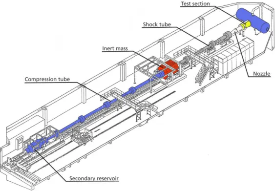
h₀≈3.3 MJ kg−1, Mach numberM=7.4 and the freestream properties temperatureT_∞=277 K and densityρ∞=11 g/m3. A schematic drawing of HEG is shown in Fig. 3.1.

Figure 3.1:Schematic drawing of the High Enthalpy Shock Tunnel Göttingen, HEG. (Source: Wagner et al. (2013))

The ramp model, consisting of a flat aluminium plate (with dimensions 80 mm×20 mm) with a sharp leading edge was placed at an angle of 15° to the flow direction. It was coated with the DLR OV322 paint (Eu-based luminophore and polyurethane (PU) binder), which had been developed in collaboration with the University of Hohenheim (Ondrus et al., 2015). The ramp model had two small holes, one for a point-wise pressure measurement (using a Kulite®piezo-resistive pressure sensor mounted below the plate in the plate holder) and one for a point-wise temperature measurement (using the coaxial thermocouple Medtherm®protruding from the holder and inserted in the ramp model hole so as to be flush-mounted with the plate surface) – see Figs. 3.2 and 3.3.

(33)

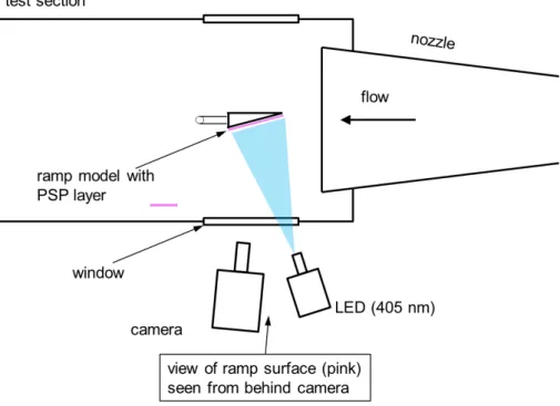
Figure 3.2:Block diagram (plan view) of experimental setup in HEG test section.

and the images were captured with a Photron® HiSpeed Camera SA1 (provided by LaVision®) running at a sampling rate of 5 kHz and with exposure times of 200 µs; recordings were carried out over 10 ms, so that 50 images in all were obtained.

Figure 3.3:Left: Detailed photograph of the ramp model, mounted in the test section. (Flow is from right to left.) Right: Photo of irradiated ramp model (pink color) in test section, showing camera and LED light source.

3.4 Temperature determination using TSP

The quenching processes which reduce the intensity of the excited paint luminophore fluorescence

(34)

obtains (Liu and Sullivan, 2005): ln I(T) I(Tre f) =Ea R 1 T − 1 Tre f (3.1) HereEais the activation energy for the non-radiative process andRis the universal gas constant. In practice, Eq. 3.1 does not always hold exactly, so that one tends (Liu and Sullivan, 2005) to carry out a calibration at knownT (andP) and perform a fit (e.g. polynomial) ofI(T)/I(Tre f)toT/Tre f:

I(Tre f)

I(T) = f(T/Tre f) (3.2)

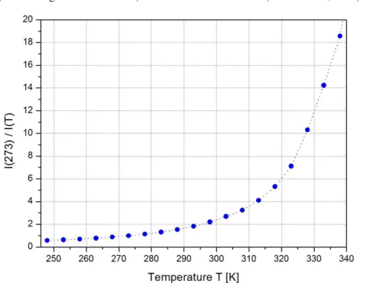
This is the standard approach adopted here, and was carried out in the laboratory using small coupons coated with the same paint as used on the test model and then calibrated in a test rig with known test conditions (viz. temperatureT and pressure p). A calibration plot for the OV322 paint used here is shown in Fig. 3.4, from which can be seen that this paint has good temperature sensitivity in the range 290 K to 340 K (ca.−3 % K−1_to_{−5 % K}−1_{(Ondrus et al., 2015).}1

Figure 3.4:Calibration of OV322 paint: intensity ratioI(273K)/I(T)vs. temperatureT. (Source: Ondrus et al. (2015).

With this calibration plot, and assuming that the conditions used in the HEG test were sufficiently similar (camera settings, lens settings, LED light source) to those of the calibration, one needs only one reference image in HEG to obtain the temperature results for all other images; these reference images in HEG are those which are obtained before gas arrival (att<1 ms) – see Fig. 3.5 and later discussion in Sects. 3.6.1 and 3.6.2.

1_{The normalization with a different temperature would also be possible, which would lead to a constant multiplicative}

(35)

3.5 Determination of heat loads

3.5.1 Temperature sensors

Measurement of heat transfer into a model surface for hypersonic flows of high enthalpy (up to 22 MJ kg−1) and short duration (down to 100 µs) places stringent requirements on the performance of the adopted temperature sensors: they must have a fast response and be able to survive the extreme environments of these flows (especially the high temperatures and, in some cases, presence of foreign particulate matter). Over the years coaxial thermoelements have become established as the sensor of choice in HEG (and most shock tunnels) to fulfil the abovementioned requirements. The firm Medtherm supplies these sensors, and also provides a calibration (see later) to be used for the evaluation of heat transfer from temperature measurements. Obviously, these sensors yield point-wise measurements only, so that a test model must be equipped with many to obtain overall heat loads; this may be difficult, especially with some complex geometries. The advantage of a field measurement technique such as TSP lies clearly to hand.

3.5.2 Evaluation of heat transfer from Medtherms and TSP

Following an approach suggested by Schultz and Jones (1973), with a modification by Cook and Felderman (1966), two key assumptions were made to obtain a simple relationship for determining heat transfer from temperature measurements:

1. Heat transfer into the model surface (or paint) is one-dimensional; 2. The surface is assumed to be semi-infinite in depth.

Obviously these requirements are only met if the time over which measurement occurs is very short – for the typical test times in shock tunnels (<10 ms), it can be shown (Martinez Schramm et al., 2015) that these assumptions are valid. Following Hannemann and Martinez Schramm (2007) (wherein a good discussion of heat transfer measurements in shock tunnels can be found), the following equation for heat transfer has been derived:

qw(t) = r ρck π T(t) √ t + 1 2 Z t 0 T(t)−T(τ) (t−τ)3/2 dτ (3.3) whereT =measured temperature,ρ=material density;c=heat capacity;k=heat conductivity; τ =time;t=integration time step. The factorρckis also known as the thermal parameter, and is strictly a function of the (sensor) material properties only. This is not fully correct, since c

andkmay also have temperature dependence – see discussion in Sect. 3.6.4. Since there are no available calibration values forρckof the TSP paint (but see later), the approach adopted here is the following: using temperatures measured by the Medtherm sensor, and using its knownρck value (as supplied by the manufacturer:ρck=7.95×107kg2K−2s−5), determine the heat load at its position using a discretized form of Eq. 3.3. Then assume that the heat load in an adjoining interrogation region (see Fig. 3.5, to be discussed later) is the same as for the Medtherm location, so that, by adjusting (varying) theρckvalue for the TSP paint in this region, the same heat load as

(36)

for the Medtherm is determined. This is effectively an insitu calibration of the TSP paint, with the foundρckbeing assumed to be the same and applicable over all the whole coated surface.

3.6 Results and discussion

This section addresses the following: raw TSP results; TSP temperature results; TSP heat load results; an estimation of the accuracy of and uncertainties in the TSP temperature and heat load results.

3.6.1 HEG results; TSP images (raw data)

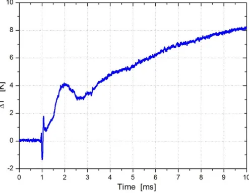
The results from only one HEG run were available, so that measurements of reproducibility could not be carried out. The temperature (Medtherm) and adjacent pressure (Kulite) measurements at the respective sensor locations (as shown in the inset in Fig. 3.5 are given in Fig. 3.7; temperature is plotted as∆T (whereT0=293 K before gas arrival) as a function of time. The bump seen peaking

at 2 ms in the Medtherm trace (also in the Kulite trace, but less marked) is due to the nozzle starting processes for this HEG condition. Fifty TSP images were recorded, one every 200 µs, over the 10 ms test time period. Fig. 3.5 shows one of these raw images (with only background correction applied, but with no correction by a reference image).

Figure 3.5:Average intensity (counts) in interrogation area vs. time (ms) for all 50 recorded raw images. Intensity and time error bars – note asymmetry - for early and late times are shown. A detailed discussion about the measurement uncertainty is given in Sect. 3.6.4.3. Inset: raw unprocessed image att=1.8 ms showing interrogation area. (Flow in the image is fromrighttoleft)

(37)

As mentioned before, and for reasons alluded to there, a small (square) interrogation region close to the Medtherm sensor location was chosen; it was situated equidistant between the Medtherm and Kulite sensors, and had a size of 15×15 pixels, which corresponds to an area on the ramp of approximately 2.5 mm×2.5 mm – see inset in Fig. 3.5. The average (over all pixels) intensity in this region was determined for all 50 images, and then plotted as a function of time, as also shown in Fig. 3.5. (Intensity and time error bars – note asymmetry - for early and late times are shown: for a discussion, see Sect. 3.6.4.3.) The abscissa time zero (origin) corresponds to the arrival of the shock wave at the end of the driven section, at which time data recording is triggered. It can be seen that it takes about 1 ms for the test gas to arrive at the test section window; hence, for times less than 1 ms, the intensity is at a maximum, after which it subsequently drops as the model surface temperature increases.

The results att<1 ms will later be used as reference values, since the conditions (viz. tempera-ture) are well-known at these early times before the test gas has arrived. They will also be used to apply intensity distribution corrections to the results att>1 ms, allowing for various geometrical effects (camera angle and settings), and for the uneven LED illumination – see Sect. 3.5.2. Interest-ingly, the bump seen clearly in the Medtherm result att=2 ms, as referred to before (see Figs. 3.6 and 3.7), appears as a change of gradient in the TSP result att≈2.5 ms – see Fig. 3.8. This slight time shift between the Medtherm and TSP results is due to the finite response time of the TSP paint, and will be discussed in more detail in Sect. 3.6.4.3. The evolution (drop) of intensity is as expected from the model described by Eq. 3.3 and with the inherent assumptions referred to before. Note from Fig. 3.5 that the intensities after 7 ms are only about 100 counts or less, so that the accuracy of the temperature determination will be lower than at early times. This is not a serious restriction, however, since typically the customarily adopted HEG test time window lies much earlier than this (around 3 ms to 4 ms) (see for example Laurence et al. (2014)); the flow at later times may be influenced by effects such as driver gas arrival and presence of other disturbances such as boundary layer leakage, arrival of the contact surface or of the reflected expansion wave, and so is often not further considered.

The change in intensity distribution on the model surface over time, brought about by the increasing surface temperature, can be clearly seen in the four raw images shown in Fig. 3.8 for the timest=1.8 ms, 2.6 ms, 5.0 ms and 9.0 ms. As expected, the average intensity drops steadily. At this stage, however, without application of the reference image corrections referred to before, nothing can be inferred about the change of temperature as a function of time over the surface – this will be addressed in the next section. Nevertheless, one can already see some physical features: for example, a wake downstream of the Medtherm (its position is shown in Fig. 3.5), clearly visible att=2.6 ms. The wake most likely arises from the sensor being mounted not fully flush with the paint surface, but recessed slightly (by about 10 µm to 100 µm) below it.2 Note again that the results at later times are most likely subject to disturbances which influence the state of the test gas; in spite of this, the development in intensity over time all the way up to 10 ms looks reasonable and

2_{The slight dent at the sensor location is not expected to influence the temperature and heat flux measurements of}

the Medtherm sensor significantly, since the boundary layer thickness at the sensor location is expected to be at least one order of magnitude larger.

(38)

Figure 3.6:Temperature change∆T measured by a Medtherm sensor on ramp model in this HEG run.

Figure 3.7:Pressure changePmeasured by a Kulite sensor on ramp model in this HEG run.

(39)

3.6.2 TSP temperature results

Using the first four recorded images as reference (Tre f =293 K), and with the help of the calibration plot shown in Fig. 3.4, one can then obtain temperatures over the whole model surface for all remaining 46 images. Ten results at different times (0.4 ms, 2 ms, 3 ms, 4 ms, 5 ms, 6 ms, 7 ms, 8 ms, 9 ms and 10 ms) are shown in Fig. 3.9, where the first image (att=0.4 ms) is a typical reference image before gas arrival. (The apparent asymmetry (e.g. see direction of the streak wakes) is due to non-parallel alignment of the wedge relative to the flow direction, which can already be inferred from the non-horizontal orientation of the raw images seen in Figs. 3.5 and 3.8.)

Figure 3.8:Average intensity (counts) in interrogation region vs. time (ms) for all 50 recorded raw images, showing four sample raw intensity images at times shown. (Flow in these images is fromrighttoleft)

Quite clearly one can see the development of temperature on the surface over time. (The result at t=0.4 ms corresponds to a reference image, viz. before gas arrival.) Results fort>5 ms suggest temperatures in excess of 330 K close to the leading edge; these lie outside the calibration range, so that the TSP results close to the leading edge for these late times can only be seen as semi-quantitative. However, it should be noted that the used TSP has been shown to work up to 380 K in a laboratory environment (Ondrus et al., 2015).

One can now plot the obtained average TSP temperatures in the interrogation region (referred to before) for all 46 images and compare the temperature development with the Medtherm results – this comparison is shown in Fig. 3.10. (Temperature and time error bars for early and late times are shown: for a discussion, see later.) Even though the TSP results aftert=2.5 ms look good and follow the expected trend, nevertheless recall the remarks made earlier. The difference in development of the actual temperature values obviously arises from the vastly different thermal

(40)

Figure 3.9:TSP temperature results (2D images) over the whole model surface for 10 different times during the HEG run. (Flow in these images is fromrighttoleft)

properties (ρck) of the Medtherm and TSP paint. This becomes clear from Table 3.1, whereρ,cand

kvalues (Eng, 2015) for three typical materials are listed, along with the productsρckand(ρck)1/2 - recall the presence of(ρck)1/2in Eq. 3.3. These materials have been chosen as ‘representative’:

Al represents the test model material, Ni the Medtherm and PMMA (polymethylmethacrylate, a polymer commonly used in TSP) the paint. The values of (ρck) and(ρck)1/2for the Medtherm, as supplied by the manufacturer, are also shown. (An aside: note that Ni has different (ρck) values to that of the Medtherm. This is not surprising, since the Medtherm is not made of just Ni, and some abraded dust from its test preparation has also been rubbed into the sensor.) The final row shows the values of(ρck)1/2for the various materials normalized to the value(ρck)1_PMMA/2 . As can be seen, mainly the much smaller k (heat conductance) value for PMMA compared with the other three materials leads also to the vastly different(ρck)1/2values – factors are up to about 40 times larger. The polymer based paint (represented by PMMA in Table 3.1) cannot conduct away the absorbed heat quickly enough, so that the paint surface heats up to higher values compared to those measured by the Medtherm.

3.6.3 TSP heat load results

Using the discretized form of Eq. 3.3 referred to before, the TSP temperature results shown in Fig. 3.9 can now be processed to give the heat loads on the model surface. This local heat load can be determined from the Medtherm measurement at its position (see Fig. 3.5 for location), so that the TSP average temperatures over time in the adjacent interrogation region can be used to determine a local heat load from TSP measurements, withρckinsitubeing varied as a parameter to

yield the same heat load from both the TSP and the adjacent Medtherm measurements – this is effectively an insitu calibration of the TSP paint using the Medtherm. The value obtained for the TSP paint with this approach wasρckinsitu=4.5×106kg2K−2s−5. It is again assumed that this

(41)

Figure 3.10:Medtherm and adjacent TSP temperatures vs. time in the HEG run, the latter using TSP calibration data. (Average TSP temperature in the interrogation area – see Fig. 3.5.)

value ofρckpertains over the whole model surface and over the whole time, so that heat loads for all 46 images (fromt=1 ms to 10 ms) over the whole ramp surface can be obtained. (The validity and inherent uncertainties of this assumption will be further discussed in Sect. 3.6.4.) Ten sample heat load results at different times (0.4 ms, 2 ms, 3 ms, 4 ms, 5 ms, 6 ms, 7 ms, 8 ms, 9 ms and 10 ms), as already shown for temperatures in Fig. 3.9, are shown in Fig. 3.11. (For the image before gas arrival att=0.4 ms the heat load is obviously zero.) Note that maximum heat loads of 1.6 MWm−2and more are obtained in the upstream (right hand side) positions on the model, even at earlier times (but recall earlier comments on paint calibration and possible damage).

As before with temperature (Fig. 3.10), one can now compare the heat load obtained from Medtherm with that from TSP in its adjacent interrogation region. This comparison is shown in Fig. 3.12. (Average error bars in time and heat transfer are shown: see discussion later.)

Here, at times aftert≈3 ms (i.e. after the initial disturbances seen in the Medtherm results), both heat load results are the same over all times and have average values of 0.73±0.07 MWm−2 for TSP and 0.70±0.08 MWm−2for Medtherm. But recall: this must obviously be so, since the Medtherm results had been used to calibrate the TSP, so that the agreement has been ‘forced’. Nevertheless, the constancy and agreement of heat loads over the whole time for both TSP and Medtherm is very encouraging. The bump in the Medtherm result att=1.6 ms to 2.0 ms correlates well with the smaller one in the TSP result att=2 ms when one considers the TSP negative time correction of 0.4 ms due to the finite paint response time – this will be discussed later in Sect. 3.6.4.

(42)

Table 3.1:Comparison of material properties (ρ density,cheat capacity,kheat conductance) and the thermal parameter(ρck)1/2for nickel Ni (representing the Medtherm thermoele-ment), aluminum Al (test model) and PMMA (a typical TSP paint polymer). (Source: see text)

Property Units Medtherm Ni Al PMMA

Densityρ kg/m3 - 8800 2712 950 Heat capacity Jkg−1K−1 - 540 870 1450 Heat conductance Js−1K−1m−1 - 90 110 0.18 ρck J 2_m−4_K−2_s−1 7.95×107 ₄_.₃_×₁₀8 ₂_.₆_×₁₀8 ₂_.₅_×₁₀5 (kg2K−2s−5) p ρck Jm −2_K−1_s−1/2 8915 20 700 16 000 500 (kgK−1s−5/2) p ρck/p(ρck)_PMMA - 18 41 32 1

3.6.4 Accuracy of TSP temperature and heat load results

Here an attempt will be made to address and identify possible sources of errors leading to uncer-tainties in the derived temperature and heat load results. These sources are both systematic and random. The final goal will be to determine confidence limits for these measured properties; they have already been shown in the foregoing plots as error bars. Specific other sources such as stray illumination (considered the major problem with quantitative TSP in shock tunnels) and particles (as dust) are not considered explicitly here; they have been discussed elsewhere (Beck et al., 2015). However, for the HEG run condition chosen here (lowh0, lowρ∞), the influence of these sources

was minimal and could therefore be neglected here.

3.6.4.1 Thermal parameterρck: material properties

The TSP paint consists of three layers sprayed onto an aluminum substrate: the bottom primer layer, a screen layer and finally the active layer consisting of the polymer (here PU) with its embedded luminophores (Eu complex). Sottong (DLR Cologne, private communication (2015)) carried out material and thermal analyses of the aluminum substrate and these three layers. Each layer thickness and thence its density were determined; Fig. 3.13 shows a scanning electron microscope (SEM) image of a sectional cut through the aluminum substrate and its paint coatings, showing the thicknesses of the three layers and the structure of their surfaces. Heat conductance coefficientsk

for the layers and substrate at temperatures from 25◦C to 50◦C were also measured; these values fork(in Wm−1K−1) are plotted as a function of temperature in Fig. 3.14. The coefficientkfor aluminum is much larger than that for the active layer, by a factor of about 100. However, in the previous estimate ofkin Table 3.1, the factor was more like 600 (≈110/0.18), which is obviously a huge over-estimate, based on these new measurement results. The conclusion remains the same, however: the main driving force for the different response of the Medtherm and TSP paint to an externally applied heat load is the large difference ink. The largest temperature dependence is