Forecasting with DSGE models

Working PaPer SerieS

no 1185 / May 2010

ForecaSting

With DSge

MoDelS

By Kai Christoffel,

Günter Coenen and

Anders Warne

W O R K I N G PA P E R S E R I E S

N O 118 5 / M AY 2 010

In 2010 all ECB publications feature a motif taken from the €500 banknote.

FORECASTING WITH DSGE MODELS

by Kai Christoffel, Günter Coenen,

and Anders Warne

1 The paper is in preparation for appearing as a chapter in an ‘Oxford Handbook’ on Economic Forecasting, edited by Michael P. Clements and David F. Hendry. We have received valuable comments and suggestions by the editors and an anonymous referee of the Handbook chapter. We are particularly grateful to Marta Bańbura who has estimated and computed the forecasts for the two large Bayesian VAR models we have used in the paper. We have received valuable comments from participants at the 2009 Nottingham workshop on DSGE modelling, seminar participants at the Humboldt University in Berlin, December 2009, and participants in the meeting of the Ökonometrie-Ausschuss des Vereins für Socialpolitik in Rauischholzhausen, March 2010. We are very grateful for discussions with and comments from Richard Anderson, Michael Burda and Alexander Meyer-Gohde. Any remaining errors are the sole responsibility of the authors. 2 All authors: Directorate General Research, European Central Bank, Kaiserstrasse 29, 60311 Frankfurt am Main, Germany; e-mail: [email protected], [email protected], This paper can be downloaded without charge from http://www.ecb.europa.eu or from the Social Science

Research Network electronic library at http://ssrn.com/abstract_id=1593643.

NOTE: This Working Paper should not be reported as representing the views of the European Central Bank (ECB). The views expressed are those of the authors and do not necessarily reflect those of the ECB.

© European Central Bank, 2010 Address

Kaiserstrasse 29

60311 Frankfurt am Main, Germany

Postal address

Postfach 16 03 19

60066 Frankfurt am Main, Germany

Telephone +49 69 1344 0 Internet http://www.ecb.europa.eu Fax +49 69 1344 6000

All rights reserved.

Any reproduction, publication and reprint in the form of a different publication, whether printed or produced electronically, in whole or in part, is permitted only with the explicit written authorisation of the ECB or the author(s).

Information on all of the papers published in the ECB Working Paper Series can be found on the ECB’s website, http://www. ecb.europa.eu/pub/scientific/wps/date/ html/index.en.html

Abstract 4

Non-technical summary 5

1 Introduction 7

2 The New rea- ide odel of the euro area 9

2.1 A bird’s eye view on the model 9

2.2 Some key model equations 10

3 Bayesian estimation of DSGE models 13

3.1 Methodology 13

3.2 Data and shock processes 14

3.3 Empirical results 16

4 Bayesian forecasting by sampling the future 17

4.1 Estimating the predictive distribution

of a DSGE model 17

4.2 Alternative forecasting models 19

5 Evaluating forecast accuracy 23

5.1 Point forecasts 23

5.2 Density forecasts 27

5.3 Relating the forecast performance

of the DSGE model to its structure 31

6 Summary and conclusions 33

Appendices 35

Figures and tables 39

References 48

CONTENTS

Abstract: In this paper we review the methodology of forecasting with log-linearised DSGE

models using Bayesian methods. We focus on the estimation of their predictive distributions, with special attention being paid to the mean and the covariance matrix ofh-step ahead fore-casts. In the empirical analysis, we examine the forecasting performance of the New Area-Wide Model (NAWM) that has been designed for use in the macroeconomic projections at the Euro-pean Central Bank. The forecast sample covers the period following the introduction of the euro and the out-of-sample performance of the NAWM is compared to nonstructural benchmarks, such as Bayesian vector autoregressions (BVARs). Overall, the empirical evidence indicates that the NAWM compares quite well with the reduced-form models and the results are there-fore in line with previous studies. Yet there is scope for improving the NAWM’s there-forecasting performance. For example, the model is not able to explain the moderation in wage growth over the forecast evaluation period and, therefore, it tends to overestimate nominal wages. As a consequence, both the multivariate point and density forecasts using the log determinant and the log predictive score, respectively, suggest that a large BVAR can outperform the NAWM.

Keywords:Bayesian inference, DSGE models, euro area, forecasting, open-economy macroe-conomics, vector autoregression.

Non-Technical Summary

Since the turn of the century, we have witnessed the development of a new generation of dynamic stochastic general equilibrium (DSGE) models that build on explicit micro-foundations with optimising agents. Major advances in estimation methodology allow the estimation of variants of these models that are able to compete, in terms of data coherence, with more standard time series models, such as vector autoregressions (VARs); see, among others, the empirical models in Christiano, Eichenbaum, and Evans (2005), Smets and Wouters (2003, 2007), Adolfson, Laséen, Lindé, and Villani (2007), and Christoffel, Coenen, and Warne (2008). Accordingly, the new generation of DSGE models provides a framework that appears particularly suited for evaluating the consequences of alternative macroeconomic policies; see, e.g., the historical overviews in Galí and Gertler (2007) and Mankiw (2006).

Efforts have also been undertaken to bring these models to the forecasting arena. Results in Smets and Wouters (2004) suggest that the new generation of closed-economy DSGE models compare well with conventional forecasting tools such as VAR models; see also Rubaszek and Skrzypczyński (2008) and Edge, Kiley, and Laforte (2009) for studies using real time data, and Wang (2009) for a forecast comparison with the factor models popularised by Stock and Watson (2002a,b). Similarly, the study by Adolfson, Lindé, and Villani (2007) shows that open-economy DSGE models can also compete well with reduced-form models; see also Adolfson, Laséen, Lindé, and Villani (2008) and Lees, Matheson, and Smith (2010). While the evidence collected in these studies indicates that DSGE models may be taken seriously from a forecasting perspective, it should be kept in mind that the number of studies is still quite limited and that the forecast samples considered do not cover events, such as a deep recession, that are particularly difficult to foresee.

Against this background, the goal of the current paper is to review and illustrate the method-ology of forecasting with DSGE models using Bayesian methods. We limit the scope of the paper to log-linearised DSGE models, and, hence, we do not consider DSGE models based on higher-order approximations, as in Fernández-Villaverde and Rubio-Ramírez (2005). We illustrate the tools discussed in the paper by applying them to a particular DSGE model. We have selected the New Area-Wide Model (NAWM), developed at the European Central Bank (ECB), which is designed for use in the (Broad) Macroeconomic Projection Exercises regularly undertaken by ECB/Eurosystem staff and for policy analysis; cf. Christoffel, Coenen, and Warne (2008). The specification of the NAWM was influenced by both economic and statistical criteria. For example, impulse-response functions and forecast-error-variance decompositions were used for assessing alternative specifications from an economic perspective, while the marginal likelihood and comparisons between model-based sample moments and estimates from the data were ap-plied as statistical model evaluation criteria. In addition, a small forecast evaluation exercise was conducted, but it was treated as one among many criteria for assessing the performance of

the model. Here we extend the forecast evaluation exercise to the full set of the NAWM’s en-dogenous variables. The forecast sample covers the period following the introduction of the euro and focuses on the 12 observed variables in the NAWM that are endogenously determined by the model. We shall study both point and density forecasts from 1 up to 8 quarters ahead. The DSGE model forecasts are compared to those from a VAR and three Bayesian VARs (BVARs), as well as the naïve random walk and (sample) mean benchmarks. We shall also consider differ-ent subsets of the observed variables included in the NAWM, as well as differdiffer-ent transformations of these variables.

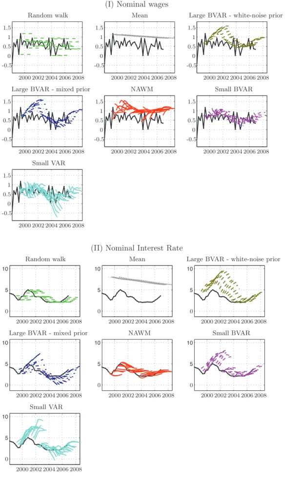
Overall, the results suggest that the NAWM performs quite well when compared with the reduced-form forecasting tools. In particular, the model compares favourably when forecasting real GDP growth, the trade variables, employment, the real exchange rate, and the short-term nominal interest rate. However, the NAWM is less successful when forecasting certain nominal variables, in particular nominal wage growth. One explanation for this is that the year-on-year steady-state growth of nominal wages is 3.1 percent in the NAWM, while wage moderation over the forecast evaluation period has kept nominal wage growth down at around 2.3 percent. The relatively strong mean reversion properties of the model therefore lead to persistent negative forecast errors.

Nevertheless, the results in this paper support earlier studies of the forecasting ability of DSGE models. At this stage of their development, they can compete when we use out-of-sample forecast performance as a measure of fit. Naturally, this does not mean that they necessarily “win” forecasting competitions in all dimensions. Moreover, it has been emphasised by, e.g., Granger (1999) and Clements and Hendry (2005) that forecast performance is not a good instrument for evaluating models in general, except when the model is intended for forecasting.

Still, the forecasting performance of the NAWM in this study is quite impressive. Yet, it is important to recall that a DSGE model—like all macroeconomic models—is a simplification of an actual economy and is therefore, one may argue, misspecified. Nevertheless, forecasting (and policy analysis) with false restrictions may not hurt the performance of a model and, as pointed out by, e.g., Sims (1980), they may even help a model to function for these purposes when the restrictions are not “very false”. The degree to which such misspecification matters may be diagnosed by making use of tools that allow us to study departures from the restrictions implied by the model. With the aid of one such tool, the so-called DSGE-VAR, Del Negro, Schorfheide, Smets, and Wouters (2007) note that misspecification of the DSGE model they estimate is not so large as to prevent its use in policy analysis. Not least in view of the findings in this article, the extent to which possible misspecification matters for the NAWM is an important question that we shall examine in a future study of the model.

Structural econometric forecasting, because it is based on explicit theory, rises and falls with the theory, typically with a lag.

Francis X. Diebold (1998, p. 175).

1. Introduction

Since the turn of the century, we have witnessed the development of a new generation of dynamic stochastic general equilibrium (DSGE) models that build on explicit micro-foundations with optimising agents. Major advances in estimation methodology allow the estimation of variants of these models that are able to compete, in terms of data coherence, with more standard time series models, such as vector autoregressions (VARs); see, among others, the empirical models in Christiano, Eichenbaum, and Evans (2005), Smets and Wouters (2003, 2007), Adolfson, Laséen, Lindé, and Villani (2007), and Christoffel, Coenen, and Warne (2008). Accordingly, the new generation of DSGE models provides a framework that appears particularly suited for evaluating the consequences of alternative macroeconomic policies; see, e.g., the historical overviews in Galí and Gertler (2007) and Mankiw (2006).

Efforts have also been undertaken to bring these models to the forecasting arena. Results in Smets and Wouters (2004) suggest that the new generation of closed-economy DSGE models compare well with conventional forecasting tools such as VAR models; see also Rubaszek and Skrzypczyński (2008) and Edge, Kiley, and Laforte (2009) for studies using real time data, and Wang (2009) for a forecast comparison with the factor models popularised by Stock and Watson (2002a,b). Similarly, the study by Adolfson, Lindé, and Villani (2007) shows that open-economy DSGE models can also compete well with reduced-form models; see also Adolfson, Laséen, Lindé, and Villani (2008) and Lees, Matheson, and Smith (2010). While the evidence collected in these studies indicates that DSGE models may be taken seriously from a forecasting perspective, it should be kept in mind that the number of studies is still quite limited and that the forecast samples considered do not cover events, such as a deep recession, that are particularly difficult to foresee.

Against this background, the goal of the current paper is to review and illustrate the method-ology of forecasting with DSGE models using Bayesian methods. We limit the scope of the paper to log-linearised DSGE models, and, hence, we do not consider DSGE models based on higher-order approximations, as in Fernández-Villaverde and Rubio-Ramírez (2005). As regards the initial steps of forecasting with DSGE models, Sargent (1989) was amongst the first to point out that a log-linearised DSGE model can be cast in the familiar state-space form, where the ob-served variables are linked to the model variables (and possibly to measurement errors) through the measurement equation. At the same time, the state equation provides the reduced form of the DSGE model, mapping current model variables to their lags and the underlying i.i.d. shocks, where the reduced form is obtained by solving for the expectation terms in the structural form of the model using a suitable method; see, e.g., Blanchard and Kahn (1980), Anderson and Moore (1985), Anderson (2010), Klein (2000), or Sims (2002). The Kalman filter can thereafter be used

to compute the value of the log-likelihood function for any value of the model parameters when a (unique) solution of the DSGE model exists. A classical approach to the estimation of these parameters would then be to maximise the log-likelihood function with numerical methods. A Bayesian approach would instead complement the likelihood with a prior distribution for the parameters and estimate the posterior mode through numerical optimisation, or other properties of the posterior distribution via Markov Chain Monte Carlo (MCMC) methods.

In this paper, we shall discuss an algorithm for estimating the predictive distribution of the observed variables based on draws from the posterior distribution of the DSGE model param-eters and simulation of future paths for the variables with the model. The general method, called sampling the future, was first suggested for univariate time series models by Thompson and Miller (1986). Their variant was simplified and adapted to VAR models by Villani (2001). The particular version of the algorithm that can be used for state-space models was suggested in Adolfson, Lindé, and Villani (2007). If the forecast evaluation exercise only requires moments from the predictive distribution, such as the mean and the covariance, then the simulation al-gorithm is not necessary. Estimation of such moments can instead be achieved by properly combining population moments for fixed parameter values with draws from the posterior dis-tribution and, thus, without sampling the future via the model. However, if we also wish to estimate, e.g., quantiles, confidence intervals or the probability that the variables reach some barrier, then the simulation algorithm may prove useful. We note that the algorithm does not rely on a particular posterior sampler. It only requires that a sufficiently large number of random draws is available from the posterior distribution of the parameters.

We illustrate these tools by applying them to a particular DSGE model. We have selected the New Area-Wide Model (NAWM), developed at the European Central Bank (ECB), which is designed for use in the (Broad) Macroeconomic Projection Exercises regularly undertaken by ECB/Eurosystem staff and for policy analysis. The specification of the NAWM was influ-enced by both economic and statistical criteria. For example, impulse-response functions and forecast-error-variance decompositions were used for assessing alternative specifications from an economic perspective, while the marginal likelihood and comparisons between model-based sam-ple moments and estimates from the data were applied as statistical model evaluation criteria. In addition, a small forecast evaluation exercise was conducted, but it was treated as one among many criteria for assessing the performance of the model. Here we extend the forecast evaluation exercise to the full set of the NAWM’s endogenous variables. The forecast sample covers the period following the introduction of the euro and we shall study both point and density fore-casts from 1 up to 8 quarters ahead. The DSGE model forefore-casts are compared to those from a VAR and three Bayesian VARs (BVARs), as well as the naïve random walk and (sample) mean benchmarks. We shall also consider different subsets of the observed variables included in the NAWM, as well as different transformations of these variables.

The remainder of the paper is organised as follows. Section 2 sketches the NAWM, while Section 3 reports on our implementation of Bayesian inference methods and on some selected estimation results for the NAWM. Section 4 first discusses how the predictive distribution of a DSGE model can be estimated, and it then presents the alternative forecasting models that are used in the empirical analysis. Section 5 covers the forecast evaluation of the NAWM, focusing first on point forecasts and then on density forecasts. Section 6 summarises the main findings of the paper and concludes.

2. The New Area-Wide Model of the Euro Area

In this section we provide a brief overview of the NAWM to set the stage for our review of the methodology for forecasting with log-linearised DSGE models. The NAWM is a micro-founded open-economy model of the euro area designed for use in the ECB/Eurosystem staff projections and for policy analysis; see Christoffel, Coenen, and Warne (2008) for a detailed description of the NAWM’s structure. Its development has been guided by a principal consideration, namely to provide a comprehensive set of core projection variables, including a number of foreign variables, which, in the form of exogenous assumptions, play an important role in the projections. As a consequence, the scale of the NAWM—compared with a typical DSGE model—is rather large, and it is estimated on 18 macroeconomic time series.

2.1. A Bird’s Eye View on the Model

The NAWM features four classes of economic agents: households, firms, a fiscal authority and a monetary authority. Households make optimal choices regarding their purchases of consumption and investment goods, they supply differentiated labour services in monopolistically competitive markets, they set wages as a mark-up over the marginal rate of substitution between consumption and leisure, and they trade in domestic and foreign bonds.

As regards firms, the NAWM distinguishes between domestic producers of tradeable differen-tiated intermediate goods and domestic producers of three types of non-tradeable final goods: a private consumption good, a private investment good, and a public consumption good. The intermediate-good firms use labour and capital as inputs to produce their differentiated goods, which are sold in monopolistically competitive markets domestically and abroad. Accordingly, they set different prices for domestic and foreign markets as a mark-up over their marginal costs. The final-good firms combine domestic and foreign intermediate goods in different proportions, acting as price takers in fully competitive markets. The foreign intermediate goods are imported from producers abroad, who set their prices in euros, allowing for an incomplete exchange-rate pass-through. A foreign retail firm in turn combines the exported domestic intermediate goods, where aggregate export demand depends on total foreign demand.

Both households and firms face nominal and real frictions, which have been identified as im-portant in generating empirically plausible dynamics. Real frictions are introduced via external

habit formation in consumption and through generalised adjustment costs in investment, im-ports and exim-ports. Nominal frictions arise from staggered price and wage-setting à la Calvo (1983), along with (partial) dynamic indexation of price and wage contracts. In addition, there exist financial frictions in the form of domestic and external risk premia.

The fiscal authority purchases the public consumption good, issues domestic bonds, and levies different types of distortionary taxes. Nevertheless, Ricardian equivalence holds because of the simplifying assumption that the fiscal authority’s budget is balanced each period by means of lump-sum taxes. The monetary authority sets the short-term nominal interest rate according to a Taylor-type interest-rate rule, with the objective of stabilising inflation in line with the ECB’s definition of price stability.

The NAWM is closed by a rest-of-the-world block, which is represented by a structural VAR (SVAR) model determining a small set of foreign variables: foreign demand, foreign prices, the foreign interest rate, foreign competitors’ export prices and the price of oil. The SVAR model does not feature spill-overs from the euro area, in line with the treatment of the foreign variables as exogenous assumptions in the projections.

2.2. Some Key Model Equations

To better understand the cross-equation restrictions implied by the NAWM’s structure, it is instructive to look at some key behavioural equations in their log-linearised form. We focus on those equations most closely related to the set of 12 observed variables that form the basis of the forecasting performance evaluation in Section 5; namely, private consumption, investment, imports and exports, the private consumption and the import deflator, wages and employment, the short-term nominal interest rate and the real effective exchange rate. Real GDP and the GDP deflator are obtained from the model’s aggregate resource constraint in real and in nominal terms, respectively.

In order to derive the log-linearised equations, the NAWM is first cast into stationary form. To this end, all real variables are measured in per-capita terms and scaled by trend labour productivity z_t. This variable is assumed to follow a random walk with stochastic drift and defines the model’s balanced growth path. Similarly, we normalise all nominal variables with the price of the consumption goodP_C,t. For example, we usec_t=C_t/z_tto denote the stationary level of per-capita consumption, while we usep_I,t=P_I,t/P_C,t to represent the stationary relative price of the investment good. We then proceed with the log-linearisation of the transformed NAWM around its deterministic steady state, where the logarithmic deviation of a variable from its steady-state value is denoted by a hat (‘’). For example, the log-deviation from steady state for the scaled consumption variable isc_t= log(c_t/c).

With these conventions, private consumptionc_tis characterised by an intertemporal optimal-ity condition (Euler equation), which relates the log-difference of current and expected future consumption to the ex-ante real interest rate, r_t−Et[πC,t+1], noting that the specific form of

that lagged consumption also enters the consumption equation: c_t = 1 1 +κgz−1 E_t[c_t+1] + κg −1 z 1 +κgz−1 c_t−1−1−κg −1 z 1 +κgz−1 r_t−E_t[π_C,t+1] +RP_t (1) − 1 1 +κg−_z1 Et[gz,t+1]−κgz−1gz,t . Here, RP

t denotes a risk-premium shock, which drives an exogenous wedge between the riskless

interest rate set by the monetary authority and the effective interest rate faced by households. The expected quasi-difference of trend labour productivity growth, E_t[g_z,t+1]−κg_z−1g_z,t, enters as an additional term because of the scaling of the consumption variable with the level of trend productivity, where g_z denotes the steady-state value ofg_z,t=z_t/z_t−1.

Investmenti_tis characterised by an equation with a similar structure. The intertemporal price of investment is given by the log-difference of Tobin’s Q—the discounted sum of expected future returns of the existing capital stock, with discount factor β—and the price of newly installed capital goods,Q_t−p_I,t:

i_t = β 1 +βEt i_t+1 + 1 1 +βit−1+ 1 γ_Ig2_z(1 +β) Q_t−p_I,t+I_t (2) + 1 1 +β βE_t[g_z,t+1]−g_z,t .

The intertemporal price of investment is shifted by an investment-specific technology shock I t,

which affects the efficiency of newly installed capital goods. The lagged investment term reflects the existence of adjustment costs related to incremental changes in investment, with sensitivity parameter γ_I.

Private consumption and investment are composed of bundles of domestic and imported intermediate goods, imC_t and imI_t. The demand for these import bundles depends on the total demand for the consumption good, qC

t = ct, and the investment good, qtI =it, respectively.

Suppressing the consumption and investment superscripts for the sake of simplicity and focusing on the generic form of the import demand equation, the share of imports in total demand is then obtained as a function of the price of the imported intermediate-goods bundle relative to the price of the generic final good,p_IM,t−p_t:

im_t = −μ p_IM,t−p_t−Γ†_{IM ,t} +q_t. (3)

Here, the parameterμrepresents the price elasticity of import demand. As in the case of invest-ment, adjustment costs are incurred which, in their generic form Γ†_{IM ,t}, dampen the influence of changes in the relative price of imports on import demand.

The demand for euro area exports x_t is determined in a similar way as a share of euro area foreign demandy∗_t. This share varies with the price of euro area exports (translated into foreign currency with the real effective exchange rate s_t, denominated in terms of the GDP deflator

p_Y,t) relative to the price of exports of the euro area’s competitors,p_X,t−s_t−p_Y,t−pc X,t: x_t = −μ∗ p_X,t−s_t−p_Y,t−pc_X,t−Γ†_X,t +y∗_t +ν_t∗, (4) where the parameterμ∗ denotes the price elasticity of exports. The termΓ†_X,trepresents generic adjustment costs, and the term ν_t∗ is an exogenous shock to foreign export preferences.

Consumer prices are determined as a combination of the aggregate prices of the domestically produced and the imported intermediate goods,p_H,tand p_IM,t. The evolution of these prices is governed, in generic form, by forward-looking Phillips-curve equations according to which the rate of price inflationπ_tgradually adjusts in response to fluctuations in real marginal costsmc_t, subject to an exogenous price mark-up shock ϕ_t:

π_t = β 1 +βχEt[πt+1] + χ 1 +βχπt−1+ (1₋βξ) (1−ξ) ξ(1 +βχ) (mct+ϕt). (5)

This equation derives from the typical Calvo assumption that firms can only infrequently re-set their prices optimally, namely with probability 1−ξ. Those firms which are not permitted to do so are allowed to index their prices to past inflation π_t−1 with indexation parameter χ.

Real wages and hours worked are the key labour-market variables in the NAWM. Real wages

w_tadjust gradually according to a forward-looking Phillips-curve equation which closes the gap between the after-tax real wage w_tτ and the marginal rate of substitution mrs_t, subject to an exogenous wage mark-up shock ϕW_t :

w_t = β 1 +βEt[wt+1] + 1 1 +βwt−1+ β 1 +βEt[πC,t+1] (6) −1 +βχW 1 +β πC,t+ χ W 1 +βπC,t−1− (1₋βξ W) (1−ξW) (1 +β)ξ W(1 + ϕW ϕW−1ζ) wτ_t −mrs_t−ϕW_t .

As in the case of the price Phillips curves, the parameters 1−ξ_W and χ_W denote, respectively, the Calvo adjustment probability for (nominal) wages and the degree of indexation to past consumer price inflation π_C,t−1. The parameterϕW _{denotes the steady-state wage markup and}

ζ the Frisch elasticity of labour supply.

Since there exist no reliable data for hours worked in the euro area, we rely on employment data and relate the employment variable E_t to the NAWM’s unobserved hours-worked variable

N_t by an auxiliary equation following Smets and Wouters (2003),

E_t = β 1 +β Et[Et+1] + 1 1 +β Et−1+ (1₋βξ E) (1−ξE) (1 +β)ξ E N_t−E_t . (7)

Here, the parameterξ

E determines the sensitivity of employment with respect to hours worked,

similar to the role of the Calvo parameters in the price and wage Phillips curves.

The monetary authority sets the short-term nominal interest rate r_t according to a simple Taylor-type interest-rate rule, where the parameter φ_R represents the degree of interest-rate smoothing and the parameters φ_Π, φ_ΔΠ and φ_ΔY determine the sensitivity of the interest-rate response to, respectively, consumer price inflation, the change in inflation and real GDP growth

(relative to trend productivity growth):

r_t = φ_Rr_t−1+ (1−φ_R)φ_Ππ_C,t−1+φ_ΔΠ(π_C,t−π_C,t−1) +φ_ΔY (y_t−y_t−1) +ηR_t . (8) The termηR

t denotes a serially uncorrelated monetary policy shock.

Finally, the real effective exchange rates_tis determined by a risk-adjusted uncovered interest parity condition: s_t = Et[st+1]−rt+r∗t −RPt +Et π_Y,t+1−π∗_Y,t+1−γ_B∗s_B∗_,t+1−RP_t ∗, (9) where r_t∗ and π∗_Y,t+1 denote the foreign interest rate and foreign inflation, respectively. The last two terms represent an external risk premium. It is composed of an endogenous component related to the net holdings of foreign bonds, s_B∗_,t+1 with sensitivity γ_B∗, and an exogenous shock RP∗

t .

The NAWM’s log-linearised equations, including the equations presented above, can be cast in state-space form, where the state equation corresponds to the reduced-form solution of the model, which we obtain using the AIM algorithm developed in Anderson and Moore (1985) and Anderson (2010). The observed variables are related to the model’s state variables through an appropriate measurement equation.

3. Bayesian Estimation of DSGE Models

We adopt the empirical approach outlined in Smets and Wouters (2003) and An and Schorfheide (2007) and estimate the NAWM employing Bayesian inference methods. This involves obtaining the posterior distribution of the model’s parameters based on its log-linear state-space represen-tation using the Kalman filter. For the empirical analyses, we use YADA, a Matlab programme for Bayesian estimation and evaluation of DSGE models; see Warne (2010).

In the following we sketch the adopted approach and describe the data and the shock processes that we consider in its implementation. We then briefly report on the calibration of the model’s steady state and present some selected estimation results.

3.1. Methodology

Employing Bayesian inference methods allows the role of prior information obtained from earlier studies, at both the micro and macro level, to be formalised in the estimation of the parameters of possibly complex DSGE models. This seems particularly appealing in situations where the sample period of the data is relatively short, as for the euro area. From a practical perspective, Bayesian inference may also help to alleviate the inherent numerical difficulties associated with solving the highly non-linear estimation problem.

Formally, let p(θ_m|m) denote the prior distribution of the vector θ_m ∈ Θ_m with structural parameters for some modelm∈ M, and letp(Y_T|θ_m, m) denote the likelihood function for the observed data, Y_T ={y₁, . . . , y_T}, conditional on parameter vectorθ_m and modelm. The joint posterior distribution of θ_m for model m is then obtained by combining the likelihood function

for Y_T and the prior distribution of θ_m,

p(θ_m|Y_T, m)∝p(Y_T|θ_m, m)p(θ_m|m),

where ∝denotes proportionality.

The posterior distribution is typically characterised by measures of location, such as the mode or the mean, measures of dispersion, such as the standard deviation, or selected quantiles. Following Schorfheide (2000), we adopt an MCMC sampling algorithm to determine the joint posterior distribution of the parameter vectorθ_m. More specifically, we rely on the random-walk Metropolis algorithm with a Gaussian proposal density to obtain a large number of random draws from the posterior distribution of θ_m. The posterior mode and the inverse Hessian matrix are computed by a standard numerical optimisation routine, namely Christopher Sims’ optimiser

csminwel.1

As discussed in Geweke (1999), Bayesian inference also provides a framework for comparing alternative and potentially misspecified models on the basis of their marginal likelihood. For a given model mthe latter is obtained by integrating out the parameter vector θ_m,

p(Y_T|m) =

θm∈Θm

p(Y_T|θ_m, m)p(θ_m|m)dθ_m.

Thus, the marginal likelihood gives an indication of the overall likelihood of the observed data conditional on a model. To estimate the marginal likelihood one may use the modified harmonic mean estimator, suggested by Geweke (1999); see also Geweke (2005). An alternative estimator, suggested by Chib and Jeliazkov (2001), relies on rewriting Bayes theorem into the so-called marginal likelihood identity. The former estimator requires only draws from the posterior ofθ_m, while the latter also requires draws of these parameters from the proposal density.

3.2. Data and Shock Processes

In estimating the NAWM, we use time series for 18 macroeconomic variables which feature prominently in the ECB/Eurosystem staff projections: real GDP, private consumption, total investment, government consumption, extra-euro area exports and imports, the GDP deflator, the consumption deflator, the extra-euro area import deflator, total employment, nominal wages per head, the short-term nominal interest rate, the nominal effective exchange rate, foreign demand, foreign prices, the foreign interest rate, competitors’ export prices, and the price of oil. All time series are taken from an updated version of the AWM database (see Fagan, Henry, and Mestre, 2005), except for the time series of extra-euro area trade data, the construction of which is detailed in Dieppe and Warmedinger (2007). The sample period ranges from 1985Q1 to 2006Q4 (using the period 1980Q2 to 1984Q4 as a training sample). The last five variables are modelled using an SVAR, the estimated parameters of which are kept fixed throughout the estimation of the NAWM. Similarly, government consumption is specified by means of an autoregressive (AR)

1_{Thecsminwelsoftware is available from Sims’ homepage athttp://sims.princeton.edu/yftp/optimize/and from}

process with fixed estimated parameters. For details, see Christoffel, Coenen, and Warne (2008, Section 3.2).

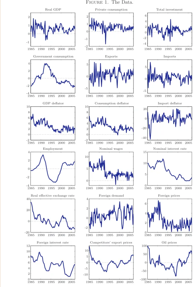
Prior to estimation, we transform real GDP, private consumption, total investment, extra-euro area exports and imports, the associated deflators, nominal wages per head, as well as foreign demand and foreign prices into quarter-on-quarter growth rates, approximated by the first difference of their logarithm. Furthermore, a number of additional transformations are made to ensure that variable measurement is consistent with the properties of the NAWM’s balanced-growth path and in line with the underlying assumption that all relative prices are stationary. First, the sample growth rates of extra-euro area exports and imports as well as foreign demand are matched with the sample growth rate of real GDP by removing the sample growth rate differentials, reflecting the fact that trade volumes and foreign demand tend to grow at a significantly higher rate than real GDP. Second, for the logarithm of government consumption we remove a linear trend consistent with the NAWM’s steady-state growth rate of 2.0 percent per annum which is assumed to have two components: labour productivity growth,

g_z, of roughly 1.2 percent and labour force growth of approximately 0.8 percent. The former is broadly in line with the average labour productivity growth over the sample period. Third, we take the logarithm of employment and remove a linear trend consistent with a steady-state labour force growth rate of 0.8 percent, noting that, in the absence of a reliable measure of hours worked, we use data on employment in the estimation. Fourth, we construct a measure of the real effective exchange rate from the nominal effective exchange rate, the domestic GDP deflator and foreign prices (defined as a weighted average of foreign GDP deflators) and then remove the mean. Finally, competitors’ export prices and oil prices (both expressed in the currency basket underlying the construction of the nominal effective exchange rate) are deflated with foreign prices before unrestricted linear trends are removed from the variables. Figure 1 shows the time series of the transformed variables for the sample period 1985Q1 to 2006Q4.

To ensure that the 1-step ahead covariance matrix in the likelihood function for the observed variables is non-singular, the NAWM features 12 distinct structural shocks, several of which have been discussed in Section 2.2 above, plus the 6 shocks in the AR and SVAR models for government consumption and the foreign variables, respectively. All shocks are assumed to follow first-order autoregressive processes, except for the monetary policy shock and the shocks in the AR and SVAR models, which are assumed to be serially uncorrelated. We recall in this context that assuming an autoregressive process for trend labour productivity growth g_z,t—referred to as the NAWM’s permanent technology shock—implies that all real variables, with the exception of hours worked and employment, share a common stochastic trend, in line with the model’s balanced-growth property.

In addition, we account for measurement error in extra-euro area trade data (both volumes and prices) in view of the fact that they are prone to revisions. We also allow for small errors in the measurement of real GDP and the GDP deflator to alleviate discrepancies between the

national accounts framework underlying the construction of official GDP data and the NAWM’s aggregate resource constraint.

3.3. Empirical Results

An extensive discussion of the empirical implementation of the NAWM is beyond the scope of this paper, and the reader is thus referred to Christoffel, Coenen, and Warne (2008) for details. Here we report selectively on the calibration of the model’s steady state and the posterior distribution of some key estimated parameters, which is deemed helpful for understanding the model’s forecasting performance analysed in Section 5.

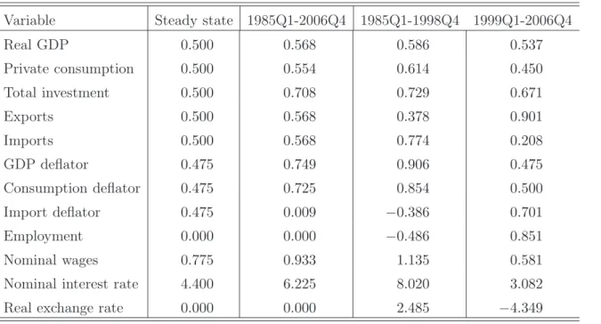
Regarding the NAWM’s steady state, all real variables are assumed to evolve along a balanced-growth path with a trend balanced-growth rate of 2 percent per annum, which roughly matches average real GDP growth in our estimation sample; see Table 1. Since the steady-state growth rate for the labour force can be seen as a proxy for population growth, all quantities within the NAWM can be interpreted in per-capita terms once it has been accounted for. Consistent with the balanced-growth assumption, we then calibrate key steady-state ratios of the model by matching their empirical counterparts over the sample period. For example, the expenditure shares of private consumption, total investment and government consumption are set to, respectively, 57.5, 21 and 21.5 percent of nominal GDP, while the export and import shares are set to 16 percent, ensuring balanced trade in steady state. On the nominal side the monetary authority’s long-run (net) inflation objective is set equal to 1.9 percent at an annualised rate, consistent with the ECB’s quantitative definition of price stability of inflation being below, but close to 2 percent. This implies that, within the NAWM, nominal wages grow with a steady-state rate of 3.1 percent, corresponding to the sum of trend labour productivity growth of 1.2 percent and the inflation objective of 1.9 percent.

As to the choice of prior distributions for the NAWM’s estimated parameters, we follow Smets and Wouters (2003) since their closed-economy model of the euro area is essentially nested within the NAWM. Our choice of prior distributions for the parameters concerning the NAWM’s open-economy dimension is informed by the priors employed in Adolfson, Laséen, Lindé, and Villani (2007). Comparing the plots of the prior and posterior distributions we find that the observed data provide additional information for most parameters. A number of estimation results are noteworthy. First, the estimates of the parameters shaping the dynamics of domestic demand in response to the model’s structural shocks—the degree of habit formation in consumption, κ, and the investment adjustment cost parameter, γ_I—are broadly in line with those reported by Smets and Wouters. Second, on the nominal side, we observe that the estimate of the Calvo parameter constraining the frequency of price-setting decisions of domestic firms selling in home markets,ξ

H, is rather high. Yet our posterior mode estimate of about 0.92 is comparable with

a point estimate of about 0.90 for the Calvo parameter in the model of Smets and Wouters. The estimate implies that the NAWM’s domestic Phillips curve is rather flat or, in other words, that the sensitivity of domestic inflation with respect to movements in real marginal cost is

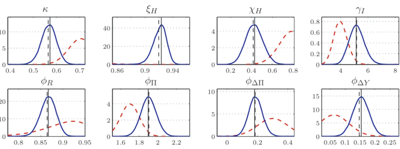
low. Similarly, the posterior mode estimate of the indexation parameterχ_His 0.42, suggesting a relatively low degree of inflation persistence. Third, regarding the interest-rate rule, we observe that the estimated response coefficientsφ_R,φ_Π,φ_ΔΠandφ_ΔY are close to the estimates reported in Smets and Wouters, despite the fact that the NAWM’s interest-rate rule does not feature a response to the so-called flex-price output gap, unlike the rule considered by Smets and Wouters. Finally, regarding the properties of the structural shocks, none of the estimated shock processes appears excessively persistent.

Figure 2 depicts the prior and posterior distributions of the structural parameters κ, γ_I,ξ_H

and χ_H, and the response coefficients of the interest-rate rule, φ_R, φ_Π, φ_ΔΠ and φ_ΔY, using the full sample, whereas Figure 3 shows the sequence of the posterior mode estimates when the sample is updated recursively over the period following the introduction of the euro. Overall, the recursively updated posterior mode estimates reveal a rather high degree of stability. Yet the gradual upward shift of the Calvo parameterξ

H suggests that domestic inflation has become

less sensitive to movements in marginal costs over time. The gradual fall in the indexation parameter χ_H implies a diminishing degree of inflation persistence, which may be interpreted as an indication that the anchoring of inflation expectations has been strengthened with the introduction of the euro area.

4. Bayesian Forecasting by Sampling the Future

4.1. Estimating the Predictive Distribution of a DSGE Model

Letθ∈Θbe the vector of parameters of the log-linearised DSGE model; to simplify notation we have omitted the modelm index in this section. Given that a unique convergent solution exists at a particular value for the parameter vector, we can express the model variables (defined as deviations from the steady state) as a VAR system. Specifically, letη_tbe aq-dimensional vector with i.i.d. standard normal structural shocks (η_t∼N(0, I_q)), whileξ_tis ther-dimensional vector of model variables, for t = 1,2, . . . , T. The solution (reduced form) of a log-linearised DSGE model can now be represented by:

ξ_t=F ξ_t−1+Bη_t, t= 1, . . . , T, (10) where F and B are uniquely determined by θ. The observed variables are denoted by y_t, an

n-dimensional vector, which is linked to the model variables ξ_t through the equation

y_t=Ax_t+Hξ_t+w_t, t= 1, . . . , T. (11) The k-dimensional vector x_t is here assumed to be deterministic, while w_t is a vector of i.i.d. normal measurement errors with mean zero and covariance matrix R. The measurement errors and the shocksη_t are assumed to be independent, while the matrices A,H, andRare uniquely determined by θ.

The system in (10) and (11) is a state-space model with ξ_t being partially unobserved state variables when, for example, r > n. Equation (10) gives the state or transition equation and (11) the measurement or observation equation. Provided the number of measurement errors and structural shocks is large enough, we can calculate the likelihood function for the observed data YT ={y1, . . . , yT} via the Kalman filter; see, e.g., Hamilton (1994) for details. The filter can

also be used to estimate all the unobserved variables in the model for a given value of θ. The predictive density ofy_T+1, . . . , y_T+H can be expressed as

p y_T+1, . . . , y_T+H|Y_T=

θ∈Θ

p y_T+1, . . . , y_T+H|Y_T, θp θ|Y_Tdθ, (12) wherep(θ|Y_T)is the posterior density of θbased on the data available at time T. If we wish to estimate quantiles, confidence regions or the probability that the variables reach some barrier, then we need a numerical algorithm for computing the predictive density since the integral in (12) cannot be solved analytically. On the other hand, if the forecast evaluation only requires moments from the predictive distribution, then such an algorithm is not needed since the mo-ments can be estimated with high precision using draws from the posterior distribution of the parameters.

A numerical algorithms for evaluating the integral in (12) for ARIMA models was suggested

by Thompson and Miller (1986). The basic idea is that M₁ paths are drawn randomly from

the densityp(y_T+1, . . . , y_T+H|Y_T, θ) for M₂ random draws ofθfrom its posterior density. This so-calledsampling the future algorithm has been adapted by Adolfson, Lindé, and Villani (2007) to state-space models. The 6 steps of the algorithm for such models are:

(1) Draw θfrom p(θ|Y_T);

(2) Draw the state variables at time T from ξ_T ∼ N(ξ_T|T, P_T|T), where ξ_T|T is the filter estimate of ξ_T and P_T|T is the covariance matrix of ξ_T given θand Y_T;

(3) Simulate a path for the state variables from (10) using the drawn value for ξ_T as the initial value and a sequence of structural shocks η_T+1, . . . , η_T+H drawn from N(0, I_q); (4) Draw a sequence of measurement errorsw_T+1, . . . , w_T+H fromN(0, R)and compute the

path for the observed variablesy_T+1, . . . , y_T+H using the measurement equation (11); (5) Repeat steps 2-4M₁ times for the sameθ;

(6) Repeat steps 1-5M₂ times.

The algorithm thus givesM =M₁M₂ paths from the predictive distribution in (12), and point and interval forecasts as well as quantiles can now be computed in a straightforward manner. Furthermore, the probability that a variable reaches some barrier during the forecast sample or that it turns at someT+h can be estimated by checking how often such a condition is satisfied for the different paths.

If the forecast evaluation exercise only requires moments from the predictive distribution, such as the mean and the covariance matrix, then the above algorithm is not needed. The population

mean of y_T+h givenY_T andθ is

Ey_T+h|Y_T, θ=Ax_T+h+HFhξ_T|T, h= 1, . . . , H. (13) To estimate the mean of the predictive distribution ofy_T+h we may simply compute the sample average of the right hand side of (13) for θ(i) _∼p(θ|Y

T), i = 1, . . . , M. By choosing M large

enough, the numerical standard error of this estimator of E[y_T+h|Y_T]is negligible. Similarly, the covariance matrix ofy_T+h conditional on Y_T and θ is

Cy_T+h|Y_T, θ=HFhP_T|T FhH+H ⎛ ⎝h j=1 Fj−1BB Fj−1 ⎞ ⎠H+R. (14)

The first term on the right hand side represents state-variable uncertainty given θ, the second term reflects uncertainty due to the structural shocks, and the third the uncertainty due to measurement errors. Following Adolfson, Lindé, and Villani (2007), the prediction covariance matrix ofy_T+h is given by

Cy_T+h|Y_T=E_T Cy_T+h|Y_T, θ+C_TEy_T+h|Y_T, θ, (15) where E_T and C_T denote the expectation and covariance with respect to the posterior of θ at time T. The second term on the right hand side of (15) measures the impact that parameter uncertainty has on theh-step ahead forecasts based on the population mean, while the first term can be decomposed into uncertainties due to unobserved state variables, structural shocks and measurement errors, where the dependence on the parameters has now been dealt with. The first term in (15) can be estimated by the sample average ofC[y_T+h|Y_T, θ(i)_{]in (14) for the M}

draws fromp(θ|Y_T), while the second term can be estimated by the sample covariance matrix of

E[y_T+h|Y_T, θ(i)]in (13) using these M draws. Again, we can choose M large enough such that the numerical standard errors of the estimators are negligible.

4.2. Alternative Forecasting Models

Sims (1980) convincingly argued that VARs provide a less restrictive environment for modelling macroeconomic time series than large-scale structural macroeconometric models, based on ‘in-credible’ identifying assumptions, that were prevalent at the time. However, while VARs often provide a reasonably good fit to macroeconomic time series data, a problem with using them is that they are not parsimonious and, hence, the number of variables that can be included is limited by a lack of long time series. To overcome this problem in forecasting situations, the so-called Minnesota prior (Doan, Litterman, and Sims, 1984) makes use of the old idea of shrink-age, a flexible method for constraining the dimension of the parameter space. Given the view that the random walk is relatively accurate for forecasting macroeconomic time series (in levels), the Minnesota prior is based on shrinking the VAR parameters towards univariate random-walk processes.

Moreover, VAR models may be considered as linear approximations of DSGE models. For instance, using the idea that VARs can be used to summarise the statistical properties of both observed time series data and data simulated from a DSGE model, Smith (1993) showed how they can serve as a device for estimating and conducting inference on structural parameters; see also Gouriéroux, Monfort, and Renault (1993). Furthermore, the state-space representation in (10)-(11) can, under certain conditions, be rewritten as an infinite order VAR model; see Fernández-Villaverde, Rubio-Ramírez, Sargent, and Watson (2007). If these conditions are not met, then the state-space representation of the DSGE model may have a VARMA representation, where the moving average term is not invertible.2

An early attempt at combining DSGE models with Bayesian VARs is Ingram and Whiteman (1994), who proposed a way of deriving priors for VARs from the economic model. This approach was further developed by Del Negro and Schorfheide (2004) into the so-called DSGE-VAR, where the DSGE model is used to determine the moments of the prior distribution of the VAR parameters using a normal/inverted Wishart form. The authors found that this model can compete in forecasting exercises with BVARs based on the Minnesota prior. Similar to the ideas in Smith (1993), they demonstrated how posterior inference about the DSGE model parameters can be conducted via the VAR by integrating out the dependence of the VAR parameters from the conditional posterior and thereby obtaining a marginal likelihood function for the parameters of the DSGE model; see also Del Negro and Schorfheide (2006, 2009). Moreover, they showed how the DSGE model can be utilised for providing identifying restrictions for the DSGE-VAR, thereby allowing for comparisons of, e.g., impulse responses between the DSGE model and the DSGE-VAR. The DSGE-VAR approach was further enriched by Del Negro, Schorfheide, Smets, and Wouters (2007) into a framework for assessing the time series fit of a DSGE model. Based on the goodness-of-fit tools they propose, the authors provide evidence that the Smets and Wouters model is misspecified when estimated on postwar U.S. data.

In this study, we shall consider two classes of BVARs, one that is intended for systems with a smaller dimension and one that has been proposed for large data sets; cf. Bańbura, Giannone, and Reichlin (2010). The usefulness of BVARs of the Minnesota type for forecasting purposes has long been recognised, as documented early on by Litterman (1986), and such models are therefore natural benchmarks in forecast evaluations. While a DSGE-VAR is also a relevant candidate forecast model, we have opted to focus on BVARs with statistically motivated priors since the latter are well established forecasting benchmarks.3 In addition to models estimated with 2_{In addition to the 18 structural shocks (18), the NAWM also has 4 i.i.d. measurement errors; cf. Section 3.2.}

The total number of shocks and errors of the NAWM is therefore greater than the number of observed variables (18), implying that the model does not satisfy the conditions in Fernández-Villaverde, Rubio-Ramírez, Sargent, and Watson (2007).

3_{While Del Negro, Schorfheide, Smets, and Wouters (2007) find that the DSGE-VAR model improves the point}

forecast accuracy relative to their DSGE model and to an unrestricted VAR, the exercise does not cover BVARs. The study by Del Negro and Schorfheide (2004) compares the DSGE-VAR to a BVAR with a Minnesota prior for the covariance matrix of the parameters, but where the mean for the first “own” lag takes into account if the corresponding variable is measured in (log) growth rates (zero mean) or in levels (unit mean). In addition, the prior on the autoregressive parameters is augmented with a proper inverted Wishart prior for the residual

Bayesian methods, we shall also consider more traditional forecasting models in our empirical exercise.

The small BVAR is based on the parameterisation and prior studied by Villani (2009). That is, we consider a VAR model with a prior on the steady-state parameters, and a Minnesota-style prior on the parameters on the lags of the endogenous variables; see also Adolfson, Lindé, and Villani (2007). For the p-dimensional covariance stationary vector z_t the VAR is given by:

z_t= Ψd_t+

k

l=1

Π_l z_t−l−Ψd_t−l+ε_t, t= 1, . . . , T. (16)

Thed-dimensional vectord_tis deterministic, and the residualsε_tare assumed to be i.i.d. normal with zero mean and positive definite covariance matrix Ω. The Π_l matrix is p×p for all lags, whileΨisp×dand measures the expected value of x_tconditional on the parameters and other information available at t= 0.

One advantage of the parameterisation in (16) is, as pointed out by Villani (2009), that the steady state (or mean) of the endogenous variables is directly parameterised via Ψ. For the standard parameterisation of a VAR model the parameters on the deterministic variables are written asΦ = (I_p−k_l=1Π_l)Ψwhend_t= 1. This makes it difficult to specify a prior onΦwhich gives rise to a reasonable prior distribution on the steady state. Moreover, when z_t is a subset of the observed variables used in the estimation of the NAWM, we can directly form a prior on the steady state ofz_t that is consistent with the steady-state prior for the NAWM as captured by a prior on A. This allows for a more balanced comparison between the models since they can share the same prior mean, or steady state, for the variables that appear in both models. The steady state in the NAWM is calibrated, while the steady-state prior covariance matrix is positive definite for the BVAR. Hence, some imbalance between the models remains for the steady-state parameters. Details on the small BVAR model specification and the computation of forecasts from the model are given in Appendix A.

In this paper, the variables in the BVAR with a steady-state prior are the same as those that were used by Smets and Wouters (2003), except for that they are measured as in the NAWM. That is, we use the following variables: real GDP growth, real private consumption growth, real total investment growth, GDP deflator inflation, employment, nominal wage growth, and the short-term nominal interest rate. Hence, two of the variables are given in levels (employment and the short-term nominal interest rate), while the remaining appear in first differences.

covariance matrix. Del Negro and Schorfheide find that the DSGE-VAR can compete with (and sometimes improve upon) the point forecasts of the BVAR. Ghent (2009) reaches a similar conclusion using the Litterman (1986) implementation of the Minnesota prior for detrended levels of U.S. data. Lees, Matheson, and Smith (2010) compare the forecast performance of a DSGE-VAR model to the Reserve Bank of New Zealand’s published forecasts as well as to those of a DSGE model and a BVAR with the same implementation of the Minnesota prior as in Del Negro and Schorfheide (2004). They find that although the forecasting performance of the DSGE-VAR is competitive with the published judgmental RBNZ forecasts, the BVAR generally outperforms both the DSGE-VAR and the Bank’s own forecasts. Moreover, the DSGE model compares well with the DSGE-DSGE-VAR, especially at longer forecast horizons.

Bańbura, Giannone, and Reichlin (2010) advocate the use of high-dimensional BVARs for macroeconomic forecasting purposes. Building on the well-known Minnesota prior and its de-velopments (Doan, Litterman, and Sims, 1984; Litterman, 1986), the authors suggest that as the dimension of the model increases, the overall shrinkage should be stronger; i.e., that the prior should be tighter. Building on this idea, the authors find that the forecasting performance of a small VAR model can be much improved upon by considering a high-dimensional VAR model (131 macroeconomic indicators). Moreover, their results suggest that forecasting performance is already substantially improved when the VAR model has 20 (carefully) selected macroeconomic variables.

We will therefore include two large BVARs that cover the same 18 variables as the NAWM in the study. That is, we letd_t= 1andz_t=y_tso thatp=nin (16). Moreover, we reparameterise the deterministic part such that we can use the constant term (Φ) instead of the steady-state term (Ψ). The VAR may therefore be expressed as:

y_t= Φ +

k

l=1

Π_ly_t−l+ε_t, t= 1, . . . , T. (17)

The prior distribution is based on the extension of the usual Minnesota prior to a nor-mal/inverted Wishart, as in Kadiyala and Karlsson (1997) and Robertson and Tallman (1999), and this prior is implemented via dummy observations (see, e.g., Lubik and Schorfheide, 2006). Additional dummy observations are added through a prior on the sum of theΠlmatrices, thereby

yielding non-zero prior correlations between the autoregressive parameters (see Sims and Zha, 1998). Details concerning the implementation of the dummy observations prior are given in Bańbura, Giannone, and Reichlin (2010); see also Appendix B below.

The BVARs differ in how the prior mean of the autoregressive parameters is treated. In both models, the prior mean of Πl for all l ≥ 2 as well as for the off-diagonal elements of Π1 are

zero. For the diagonal elements ofΠ₁, the prior mean is zero in one of the large BVAR models, henceforth the white-noise prior. The second large BVAR sets the prior mean of these diagonal elements equal to unity if the variable is measured in levels, and zero if in first differences. Below we shall refer to this as a mixed prior. Apart from these differences in the treatment of the mean, the priors of the two large BVARs differ only in terms of the numeric value given to the overall tightness hyperparameter; cf. Appendix B.

Posterior sampling is straightforward for the large BVAR models. Specifically, the marginal posterior ofΩis inverted Wishart, while the posterior distribution of (Φ,Π)conditional onΩis normal; see Appendix B for details. To sample from the joint posterior we may therefore use direct sampling; see, e.g., Geweke (2005, Chapter 4.1).

Since we will compare the forecasting performance of the NAWM with a small BVAR, we shall also estimate a VAR model for the same choice of variables inz_twith maximum likelihood, with the same lag length as all the BVARs (k = 4). Moreover, we shall check how well the DSGE model fares when comparing it to the naïve random-walk and mean benchmarks. The mean is

here estimated by the within-sample mean of the variables to be forecast. Similarly, we shall consider a random walk in the variables that are forecasted. Below we shall study the forecasting performance for both quarterly and annual changes of (a subset of) the variables that appear in first differences in the NAWM. Hence, the NAWM and the various VAR models do not change with these changes in the forecasted variables (although their forecasts are affected by it), the mean and the random-walk models do change. Accordingly, no matter which criterion is used for evaluating the forecasting performance across annual and quarterly changes, the ranking of the mean and random-walk models relative to the other models is likely to change.4

5. Evaluating Forecast Accuracy

The forecast performance of the NAWM along with the 6 reduced-form models will be assessed in this section using a rolling procedure. The parameters are estimated up to period T, when the predictive distribution of periods T + 1, . . . , T +H is to be computed, and when T is the 4th quarter of the year. WhenT corresponds to some quarter i= 1,2,3, the DSGE model and the alternative Bayesian models are estimated using data until T −i. Hence, these models are re-estimated annually. The other models are always estimated with data until periodT.

The first out-of-sample forecasts are computed for 1999Q1, i.e., the first quarter after the introduction of the euro, while the final period is 2006Q4. The length of the maximum forecast horizon, H, is 8 quarters, yielding 32 observations of the 1-step ahead forecasts and 25 of the 8-step ahead forecasts. Most variables in the NAWM, such as real GDP, are measured in first differences at a quarterly frequency. Since year-on-year changes are often of interest in practice we shall also, as mentioned above, study how the models perform when forecasting annual changes.

The forecast comparisons involve both point forecasts and density forecasts. For the point forecasts we analyse univariate and multivariate mean squared error (MSE) measures. The univariate tool is the usual root mean square error, while the trace and log determinant statistics of scaled MSE matrices for the different horizons are used when examining multivariate point forecasts. For the density forecasts we focus on the log predictive score.

5.1. Point Forecasts

Figure 4 shows the root mean squared forecast errors (RMSE) when forecasting quarterly changes of the variables in first differences. To facilitate the comparisons with the multivariate point forecast analysis below, the forecast errors have here been scaled with the estimated standard deviation of the variable over the period 1995Q1-2006Q4.

4_{If a variablex}

tappears in first differences in the NAWM,Δxt=xt−xt−1, the random-walk model for quarterly changes is simplyΔxt = Δxt−1+t, while the random-walk model for annual changes isΔ4xt = Δ4xt−1+t. The latter model can be rewritten as Δxt = Δxt−4+t. Similarly, the mean model for quarterly changes is

Δxt =μq+t, while the mean model for annual changes is Δ4xt =μa+t. The latter model can equivalently be expressed asΔxt=μa−Δxt−1−Δxt−2−Δxt−3+t.