Infrastructure Development and Economic Growth in Ethiopia
Biruk Birhanu Ashenafi (M.Sc.), Lecturer, Wolkite University, College of Business and Economics, Departmentof Economics Abstract
The study elucidates the mystery surrounding the belief that, infrastructure development induces economic growth. The relationship between infrastructure development and economic growth is investigated for Ethiopia during the period 1974/75-2014/15. Theoretically and empirically it has been tested that infrastructure affects economic growth either by reducing the cost of intermediate goods or through externality effect. To analyze the long run and short run dynamics between these variables the study applied ARDL; bounds tests, and ECM. The long run estimation shows both economic and social sector infrastructure development have a positive impact on economic growth. However, the bounds test doesn’t support the evidence that variables move together in the long run. Furthermore, the short run dynamics shows the speed of adjustment is too slow, only 6% disequilibrium corrected each year towards the long run path. Based on the findings the study highlights major issues policymakers should give due attention towards effective formulation and implementation of infrastructure development policies.
Keywords: Economic growth, Ethiopia, Infrastructure. 1. INTRODUCTION
The impact, infrastructure development played on economic growth trajectory of a country is the center of debate in academia, research and policy circle. The basic theoretical framework of the impact of public capital on economic growth was developed first by Arrow and Kurz (1970). Based on this framework, the endogenous growth literature shows that an increase in the stock of public capital can raise the steady state growth rate of output per capita, with permanent growth effects (Barro 1990, 1991, and Barro and Sala-I-Martin, 1992). Other studies focus on the differential impact of capital and current components of public spending on growth (Devarajan et al., 1996), showing a positive effect from capital expenditures and often negative effects from current or consumption expenditures.
On the other hand, such development indirectly enhances the productivity of existing resources. It can lead to “agglomeration effects” by pulling resources to the infrastructural developed areas by lowering production and distribution costs, stimulating private investment, improving labor productivity and engendering technological innovations. Therefore, in light of the considered effect of infrastructure development on economic growth, it would be imperative to extend the debate and empirically examine whether there is relationship in Ethiopian context.
The Ethiopian economy is highly characterized by following tight fiscal and monetary policy. According to Admit, et.al (2014) the government continued to pursue prudent fiscal policy better coordinated with monetary policy to combat inflation, while maintaining the momentum of spending in physical and social infrastructure.
One study examine prospects and perspective of infrastructure development and economic growth in India (Srinivasu and Srinivasa Rao, 2013), the result showed that, infrastructure is the prerequisite for the development of an economy. Moreover, infrastructure plays a crucial role in promoting economic growth and thereby contributes to the reduction of economic disparity, poverty and deprivation in a country. This study establishes the relationship empirically using growth theories and indicators of investment in transport, power, communication and informatics, education, and health which strongly influence the quality of life of the people.
Oyesiku Kayode et.al, (2013), investigated the impact of public sector investment in transport with economic growth in Nigeria. The finding revealed that transportation played an insignificant role in the determination of economic growth.
In the Ethiopian context, researches are scarce. According to Teklebirhan Alemu (2015), physical public infrastructure investment has a crowding in effect on private investment and shows significant positive impact on output growth, and above stimulate private investment both in the short and long run. Admasu Shiferaw et.al, (2013), in his study on road infrastructure and enterprise development dynamics showed that better road access increases a town’s attractiveness for manufacturing firms. The study also confirms towns with initially large number of firms continue to attract more firms, and there is a tendency towards convergence in the distribution of firms through reducing their geographic concentration. Yetnayet Ayalneh (2012), in evaluating transport network structure in Addis Ababa identified there is inadequate levels of infrastructure in parts of the current road network, particularly, the peripheral areas suffer from lack of roads and roads in the central areas have capacity limitation.
Generally, the brief review suggests that the effect of public capital or infrastructure differs across countries, regions, and sectors depending upon quantity and quality of the capital stock and infrastructure development.
Furthermore, additional source of variation is also exhibited in the theoretical framework used in the analysis (Pravakar. S, et al, 2012).
In light of the forgoing studies, studies are inconclusive. Besides, only few studies conducted in Ethiopia, which doesn’t follow a detailed econometric analysis. Therefore, this study fills the existing knowledge gap. literature on the growth effects of infrastructure has focused on one single infrastructure sector/indicator or public expenditure as proxy for infrastructure1. Since, constructing a single index of physical characteristics of widely varying types of infrastructure is a difficult task, this study develops a composite index of a stock of leading physical infrastructure indicators.
Every economy either developing or developed has two basic objectives; providing basic needs and facilities to their population and achieving higher growth rates. This paper provides an empirical result on how infrastructure affects growth and development. How infrastructure plays a dynamic role to fulfill the growth targets as well as achieving higher living standards. It provides insight for government in building infrastructure facilities from stimulating growth point of view.
The main objective of this study is to investigate the relationship between infrastructure development and economic growth in Ethiopia. More specifically, the research attempts; to examine the impact of economic and social sector infrastructure development on economic growth in the long run and short run. The conduct of the analysis is limited to the availability of data from 1974/75-2014/15 of the fiscal year, a period spanning 40 years.
1.1.A GLIMPSE AT FISCAL POLICY AND INFRASTRUCTURE DEVELOPMENT IN ETHIOPIA
Developments in the overall balance over time, particularly when related to GDP (or GNI), provide an indication of the changing impact of the government sector on the economy (IMF, 2014). The trend in budget balance, i.e., government revenue and expenditure shows the country, since 1974/75 never experiences fiscal surplus, if it has, can be used to finance productive expenditure, stabilize the economy, sustain debt and build up wealth.
On the expenditure frontier, average share of expenditure to GDP during the Dergue regime2 were 20.49% while during the Ethiopian People Revolutionary Democratic Front (EPRDF) it reaches 20.98%. To the side, percentage change in expenditure between the two regimes has shown also 3.50% decline in nominal terms at percentage point. While looking at the trend, it has grown dramatically.
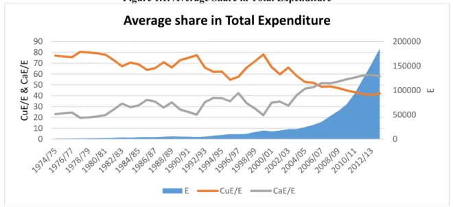
Figure 1.1. Average Share in Total Expenditure
Source: Own computation using NBE data.
Where Cu/E, CaE/E is share of recurrent and capital expenditure to total expenditure respectively. It can be evident from figure 1.1 there is huge involvement of government in the economy. In addition, over the period under review all the time expenditure exceeds revenue and even the direction of expenditure were on recurrent budget until 2006/07. It was after 2006/07 that government expenditure pattern has changed to pro-poor sectors. Thus capital expenditure share to GDP has grown significantly and the current economic growth among other factors is expected to come as a result of the development in infrastructure, education, telecommunication, energy and other allied activities.
Most literatures deal with government expenditure structure in terms of capital and current expenditure. Capital expenditure refers to those expenditures on fixed assets such as land, buildings, plant and
1Public expenditure/infrastructure investment as proxy for infrastructure development may not be right given the lack of governance and poor
outcomes of infrastructure investment in developing countries like Ethiopia.
2 The ruling regime from 1974/75-1990/91 in Ethiopia. The name Dergue means committee in local language in Ethiopia (Geez). 0 50000 100000 150000 200000 0 10 20 30 40 50 60 70 80 90 E Cu E/ E & C aE /E
Average share in Total Expenditure
machinery, which are long lasting. These are outlays on develop-mental projects that enhance the capacity of he economy for the production of goods and provision of economic and social services. Current expenditure, on the other hand, includes expenditure on wages and salaries, supplies and services, rent and so on, which are considered as consumables and recurring in the process of delivering government services (Bailey, 2002).
The average percentage share of current expenditure (CuE) to total expenditure (E) during the Dergu regime were 72.89% while under the current government witnessed 56.80%, showing a decline at 16.09% at percentage point. On the other hand the average share of capital expenditure (CaE) to total expenditure (E) before the current regime was 27.10% while under the current regime reaches at 42.21% showing an increment of 15.11% at percentage point. Moreover, the evolution of expenditure tell us, until 2005/06 the share of (CuE) to (E) has shown decline whereas the share of (CaE) to (E) shows increment. It was in 2005/06 that the two were equal and since then the share of (CaE) got a lion share.
Moreover, the two regimes under consideration has significant difference interms of the intended objectives and where the expenditure were directed. Under the Dergue regime all the time expenditure were made to recurrent budgets which means future gain from the expenditure were almost insignificant, even if, it was little. For the country once government has huge involvement in the economy it has to play in a manner that pave the way for private sectors to invest. To do that government investment in capital goods play a paramount importance. In this regard though comes latter, the current government have so much to talk about than the previous regime. And it will enhance the economy.
The study conducted by Tofik (2014), during the Dergue regime public spending had a slight increase and the real GDP too. This could mainly be due to the limited revenue source of the government as the private sector involvement in the economy, the potential tax payers, was very low due to the socialist ideology of the government. Besides, the flow of official development assistance (ODA) to the country, which is another source of revenue for the government, was very low since the then policy and ideology was not in conformity with the western states’ interest. It was after the downfall of Dergue that total public spending increased significantly following the reconstruction of the country. Spending on infrastructure development and provision of social services had grown tremendously during this period. As a result, the real GDP had registered a significant growth. The change in economic policy to a relatively free market economic system and the subsequent private sector involvement could also be the reason behind.
As mentioned earlier the country never experiences fiscal surplus since 1974/75. During the Dergue regime the share of fiscal deficit to GDP were 6.54% while during the current regime it reaches at 7.10%, so in other words the average percentage change in fiscal balance to GDP has shown 9.45% decline in nominal terms at percentage point between the two regimes. This has an implication for the usage and the direction of usage on the country’s resource. The two regimes has so much difference regarding resource mobilization and expenditure composition.
Pursuant to this change in resource mobilization and expenditure composition, the current government among the measures taken, includes changing the economy to market oriented system and made reform in diverting spending on the production of private goods and services, leaving it for the private sector towards the development of infrastructure and accumulation of capital. As a result, there was a sharp decline in the size of government expenditure as a percentage of GDP during the early post 1991/92.
Now a day’s government exert a great effort to enhance education, health, transportation and communication, energy and agricultural sector by spending great sum of money. Thus, compared to the previous regime the direction of spending in terms of principle and relevance favors the current regime. To galvanize this idea, the Dergue regime were busy to establish huge military army; thus both in theory and practices mobilizing domestic investment to defense sector has by far lower impact on growth than investing on social developments, capital goods and sectors that make the economy more integrated.
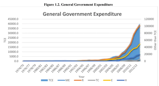
Over the past one decade one of the defining feature of Ethiopia’s economy has been huge government attention towards infrastructure development. The common argument among macroeconomist is that a large increase in public spending in infrastructure service may have a strong growth promoting effect. From 1974/75 onwards government of Ethiopia exert huge amount of money on the development of mining and energy (ME), road (R), transport and communication (TCE), health (H) and education (E). Especially during the growth and transformation periods (GTP) period providing affordable economic and social service infrastructure has given due attention in order to enhance economic growth, creating employment opportunities and expansion of industrial sector.
Figure 1.2. General Government Expenditure
Source: Own computation using NBE data.
From the above figure it is possible to observe government total capital expenditure shows a galloping increment from 2000/01. This can be justified by expenditures on main economic and social service provision sectors. For instance, average expenditure growth in mining and energy sector under the Dergu regime was 52.5% while under the current regime it accounts about 38.9%, showing a decline of 13.5% at percentage point.
The other sector that shows a tremendous positive change under the two regimes is the road sector. The average growth in road sector expenditure under the Dergu regime was 7% while under EPRDF it reached at 37.3% shows a 30.3% increment at percentage point. The transport and communication sector also be regarded as the sector that shows a positive development under the two regimes. The average growth in transport and communication sector under the Dergue regime was 53.4% but under the current regime it reached at 71% exhibited 17.6% growth at percentage point.
Social service sectors (i.e., education and health) are also important sectors that government engaged enormously for the past 40 years. In order to provide quality education to citizens both regimes in different magnitude exert huge amount of money. Under the previous regime the average growth of expenditure in education sector was 12% while under the current regime it reached at 36.5% that shows a 24.51% increase at percentage point. On the other hand, the health sector expenditure during the Dergue regime exhibited an annual growth rate average of 14.7% while under the current government it reached at 44.3% which shows 29.5% average growth at percentage point.
In nutshell total capital expenditure over the period under investigated grows on average by 20% and more specifically it has shown 6.1% increment at percentage point to the current regime. Moreover, examining the source of finance for these infrastructure development will have a paramount importance to judge the capacity of domestic economy to build infrastructure stock.
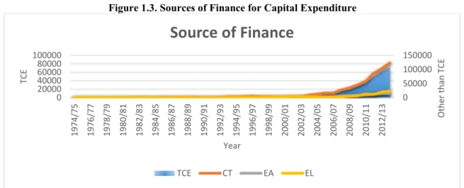
Figure 1.3, shows the source of capital expenditure for the period under investigation. As it is shown majority of capital expenditures come from central treasury, about 73% and the remaining from external loan and assistance in their order of importance. Thus, it is evident that country’s reliance in domestic capacity to develop infrastructure facilities will reduce the adverse effect of external loan.
0 20000 40000 60000 80000 100000 120000 0.0 5000.0 10000.0 15000.0 20000.0 25000.0 30000.0 35000.0 40000.0 45000.0 O th er t ha n TC E TC E Year
General Government Expenditure
Figure 1.3. Sources of Finance for Capital Expenditure
Source: Own computation using NBE data. 2. METHODOLOGY
2.1. ANALYTICAL FRAMEWORK
The linkage between infrastructure and economic growth is multiple and complex, because not only does it affect production and consumption directly, but it also creates many direct and indirect externalities, and involves large flows of expenditure thereby creating additional employment. In this framework infrastructure affects output in two ways. One is the direct channel where infrastructure increases the output by reducing the cost of intermediate goods. The other channel is through externality effect. This channel works through higher human capital returns due to education, good quality health and higher efficiency of human capital due to lower marginal depreciation of capital.
The channels through which infrastructure investment affects output and economic growth is summarized by (Seetanah, 2009). It is indicated that infrastructure development reduce the cost of intermediate goods and have a positive externality effect. This in turn improve gains in competitiveness, welfare, facilitate trade flows, improve access to school and health centers, improve environmental conditions, and reduce vulnerability of the poor. All these effects ultimately lead to improved aggregate productivity, hence, enhance economic growth. Moreover, experience across the world has shown that increase in stock of infrastructure is associated with the increase in output and the quality of life of the people.
Using theoretical framework that shows the linkage between infrastructure development and economic growth provided in the literature, the linkage often discussed in this context take the form of the following labor augmenting model. , 2.1 ; , , ! "# $$ % $ , " " & .
Equation (2.1) assumes that at any point in time, the economy has some amount of K, L, and A. so that these are combined to produce output Y. Hence, output changes overtime only if the input to production change. In particular, the amount of Y obtained from given quantities of K and L rises overtime. The model also assumes that there is technological progress only if the amount of A increases.
Since the basic motive of this study is investigating the determinants of growth, that is, how much growth over some period is due to increase in various factors of production, and how much stems from other forces; growth accounting which was pioneered by (Abramovitz, 1956; Solow, 1957), provides a basis for exploring the issue.
From equation (2.1), the growth of output can be represented as follows; Where; the dot over a variable denotes a derivative with respect to time, that is
. Dividing both sides by Y(t) and rewriting the terms on the right hand side yields.
Where; is the growth rate of O which refers to its proportional rate of change. Equation (2), is rewritten as follows; 0 50000 100000 150000 0 20000 40000 60000 80000 100000 19 74 /7 5 19 76 /7 7 19 78 /7 9 19 80 /8 1 19 82 /8 3 19 84 /8 5 19 86 /8 7 19 88 /8 9 19 90 /9 1 19 92 /9 3 19 94 /9 5 19 96 /9 7 19 98 /9 9 20 00 /0 1 20 02 /0 3 20 04 /0 5 20 06 /0 7 20 08 /0 9 20 10 /1 1 20 12 /1 3 O th er t ha n TC E TC E Year
Source of Finance
TCE CT EA ELWhere;
Finally equation (2.3) provides a way of decomposing the growth of output into the contribution of growth of capital, growth of labor, and residual.
2.2. MODEL SPECIFICATION
Following from the above analytical framework, many scholars empirically examine the contribution of infrastructure to economic growth based on the production function and closely related to a literature focused on macroeconomic role of productive public expenditure. Arrow and Kurz (1970), were the first to provide formal analysis of the effects of public capital on output.
Therefore, the econometric model adapted in this study is akin to the aforementioned researchers, by assuming a generalized Cobb-Douglas production function. The study decomposes capital investment into private capital and public capital (or Infrastructure index) as an additional input of production function along with labor force. The production function is written as follows;
'=$( )*', )+,, ', - 2.4
Where, ' # / / "/ " &0 / # / / ;
)*' % ;
)+, / ; ' $ ;
The model admits the possibility of constant or increasing returns to capital. However, shocks to infrastructure can raise the steady state income per capita in an endogenous growth model. Besides, social capital and human capital are also crucial parts of the endogenous growth model for economic growth (Lucass, 1988; Barro, 1991)1. Higher public expenditure on social infrastructure induces more literacy, better health and manpower skill, which leads to higher productivity and growth. In order to assess the impact of human capital on growth the study considers public expenditure on health and education. Hence, proxy variables is used in order to inculcating their impact on growth and provide with better insight about the role of infrastructure. In this study infrastructure development2 and economic growth is written in a semi-log linear form as follows;
Where, 1234' 1 2 3 & "/ ; 5 " 6' $ / / " 6; 77' 6 " / "/ ; 87' 6 " / ; 459:' " & % % & ; ' / $ ; ; &; 1234 #1234, 77 #77, 87 #87, 459: #459:, # . 2.3. DATA SOURCES AND DISCRIPTION
All of the data contained in the study is obtained from National Bank of Ethiopia (NBE) 1974/75-2014/15, Ministry of Finance and Economic Development (MoFED) 1974/75-2014/15, Regional Bureau’s, World Bank Africa Development Indicator Data Base 1974/75-2014/15, Ethiopian Electric Power Corporation (EEPCo), Ethiopian Road Authority (ERA), Ethiopian Airlines (EAl), Ministry of Mining and Energy (MoME). Most of the studies conducted to study the relationship between economic growth with any variables (Colombage, 2009, Koch et al., 2005, Soli et al., 2008, Karran, 1985, Hahn, 2008, Butkiewicz and Yanikkaya, 2005) used the Gross Domestic Product (GDP) as the measurement of economic growth. This study uses RGDP as a proxy of economic growth (EG) and the value of GDP (using 2010/11 as base year). Base-year analysis expresses economic measures in base-year prices to eliminate the effects of inflation.
Real Gross Domestic Product (RGDPt):- is a macroeconomic measure of the value of economic output adjusted for price changes (i.e., inflation or deflation).
Health and Education Expenditure (HEEt):- it is capital spending in both sectors to represent the development of social service infrastructure. The figure is in million birr.
1Mankiw, Romer and Weil (1992) state that: “particularly for the developing countries, investment in human capital also becomes more
quantitatively important when a more open trading environment and a better public infrastructure are in place.”
2 Infrastructure development in this study is represented by both stock and flow variables. In contrast to previous studies that assumed that
public services are derived from either flow expenditures or the stock of public capital, Tsoukis and Miller (2003) consider the case where public services are derived from both public capital stocks and expenditure flows.
Infrastructure Index (Indext):- the study develop a composite index of major infrastructure indicators to examine the impact of infrastructure development on growth. Principal Component Analysis (PCA)1 is used to create the infrastructure index by taking five major infrastructure indicators i.e., electric Power Consumption (Kwh per capita of electric consumption), energy Use (kg of oil equivalent), Telephone Subscriptions (mobile cellular subscription plus fixed subscription per 100 people), Air Transport (freight million ton-km), Road Density (the ratio of the length of the country’s total road network to the country’s land area in (sq. km)).
Private Investment (PIt):-the monetary value of private investment is used as a proxy to represent private investment.
Labor Force (LFt):- labor force is simply defined as the people who are willing and able to work. It’s the sum of male and female labor used in this study.
2.4. RESEARCH HYPOTHESIS
Regarding the long run relationship between variables; H0: There is no cointegration between series. HA: There is cointegration between series. 2.5. DATA ANALYSIS
2.5.1. UNIT ROOT ANALYSIS
Various time series techniques can be used in order to model the dynamic relationship between time series variables (Gujarati, 2004). However, it is important to determine the characteristics of the individual series before conducting further analysis. Therefore, unit root tests for stationary is examined on the levels and first differences for all variables using the most common unit root tests, which is the Augmented Dickey-Fuller (ADF). In this research the ADF test is employed since there are no missing gaps and significant structural breaks in the dataset.
2.5.2. OPTIMAL LAG LENGTH
Another key element in a model specification process is to determine the correct lag length. Several studies in this area demonstrate the importance of selecting a correct lag length. Estimates of the model would be inefficient and inconsistence if the selected lag length is different from the true lag length (Brooks, 2004). Selecting a higher order lag length than the true one over estimates the parameter values and increases the forecasting errors and selecting a lower lag length usually underestimate the coefficients and generates autocorrelated errors. Therefore, accuracy of parameters and forecasts heavily depend on selecting the true lag length. There are so many criteria used in the literature to determine the lag length of an autoregressive (AR) process. Hence, the ability to correctly locating the true lag length depends on information criterion (IC). The ordinary least Squares regression model has been run starting with lag zero upwards, since according to (Engle et al, 1995) it is the mostly used and recommended methodology used to determine the lag length. Thus, lag that provides the minimum value is chosen as the optimal lag length, in other words, among the IC that provides majority lag has been chosen as optimal lag length.
2.5.3. COINTEGRATION: AUTOREGRESSIVE DISTRIBUTED LAG MODEL (ARDL)
The autoregressive distributed lag (ARDL) model deals with single cointegration and is introduced originally by Pesaran and Shin (1999) and further extended by Pesaran et al. (2001). The ARDL approach has the advantage that it does not require all variables to be I(1) as the Johansen framework and it is still applicable if we have I(0) and I(1) variables in our set. Using bounds test method cointegration has certain econometric advantages in comparison to other methods of cointegration which are; all variables of the model are assumed to be endogenous, bounds test method for cointegration is being applied irrespectively the order of integration of the variable. There may be either integrated first order Ι(1) or Ι(0), and the short-run and long-run coefficients of the model are estimated simultaneously.
The ARDL representation of equation (2.5) is formulated as follows;
Where,
1 Principal components analysis models the variance structure of a set of observed variables using linear combinations of the variables. These
linear combinations, or components, may be used in subsequent analysis, and the combination coefficients, or loadings, may be used in interpreting the components. While we generally require as many components as variables to reproduce the original variance structure, we usually hope to account for most of the original variability using a relatively small number of component. The principal components of a set of variables are obtained by computing the eigenvalue decomposition of the observed variance matrix. The first principal component is the unit-length linear combination of the original variables with maximum variance. Subsequent principal components maximize variance among unit-length linear combinations that are orthogonal to the previous components. For additional details see Johnson and Wichtern (1992).
The left hand side is the real gross domestic product. The first until sixth expressions (β1–β6) on the right hand side correspond to the long run relationship. The remaining expressions with the summation sign (<1 <6) represent the short run dynamics of the model.
Thus, to investigate the presence of long run relationships among the lnRGDP, Index, lnEE, lnHE, lnPINV, lnLF, bound testing under Pesaran, et al. (2001) procedure is used. The bound testing procedure is based on the F-test. The F-test is actually a test of the hypothesis of no cointegration among the variables against the existence or presence of cointegration among the variables, denoted as:
H0=
HA=
The ARDL bound test is based on the Wald-test (F-statistic). The asymptotic distribution of the Wald-test is non-standard under the null hypothesis of no cointegration among the variables. Two critical values are given by Pesaran et al. (2001) for the cointegration test. The lower critical bound assumes all the variables are I(0) meaning that there is no cointegration relationship between the examined variables. The upper bound assumes that all the variables are I(1) meaning that there is cointegration among the variables. When the computed F-statistic is greater than the upper bound critical value, then the H0 is rejected (the variables are cointegrated). If the F-statistic is below the lower bound critical value, then the HA cannot be rejected (there is no cointegration among the variables). When the computed F-statistics falls between the lower and upper bound, then the results are inconclusive.
2.5.4. VECTOR ERROR CORRECTION MODEL (VECM)
Consequently, we develop the unrestricted error correction model (UECM) based on the assumption made by Pesaran et al. (2001). From the unrestricted error correction model, the long run elasticities are the coefficient of the one lagged explanatory variable (multiplied with a negative sign) divided by the coefficient of the one lagged dependent variable.
Finally, with the ARDL it is possible that different variables have differing optimal number of lags. Thus, equation (2.6) in the ARDL version of the error correction model can be expressed as equation (2.7). The error correction version of ARDL model pertaining to the variables in the former equation is as follows:
Where, is the speed of adjustment parameter; and should be negative and significant.
ECT is the residuals that are obtained from the estimated cointegration model of equation (2.6). The error correction term (ECT) contains the information of long run causality. Significance of lagged explanatory variable depicts short run causality while a negative and statistical significant ECT is assumed to signify long run causality.
The size of the coefficient is an indication of the speed of adjustment towards equilibrium in that;
• Small values of tending to -1, indicate that economic agents remove a large percentage of disequilibrium in each period.
• Larger values, tending to 0, indicate that adjustment is slow.
• Extremely small values, less than -2, indicate an overshooting of economic equilibrium. • Positive values would imply that the system diverges from the long-run equilibrium path. 3. RESULT AND DISCUSSION
3.1. Unit Root Test Results
One of the major problems encountered in studying economic relationships is the likelihood of spurious regression (seemingly related variables). To deal with this problem it is crucial to study the long run relationship of the variables. This is often done by checking if the variables are cointegrated. The first step in cointegration analysis is studying the order of integration of the variables under consideration. The order of integration of the variables in this study is determined using unit root tests.
Both from economic theories and practices for all the variables (i.e., real GDP, infrastructure index, education expenditure, health expenditure, private investment, and labor force) we can expect an increasing and decreasing trend. The trend properties of the data will determine the form of the test regression used. Thus, the test regression onwards must include a constant and trend to capture the deterministic trend. The following table revealed the ADF test results.
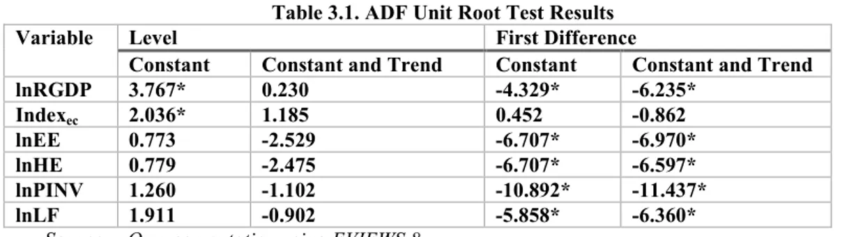
Table 3.1. ADF Unit Root Test Results
Variable Level First Difference
Constant Constant and Trend Constant Constant and Trend
lnRGDP 3.767* 0.230 -4.329* -6.235* Indexec 2.036* 1.185 0.452 -0.862 lnEE 0.773 -2.529 -6.707* -6.970* lnHE 0.779 -2.475 -6.707* -6.597* lnPINV 1.260 -1.102 -10.892* -11.437* lnLF 1.911 -0.902 -5.858* -6.360*
Source: - Own computation using EVIEWS 8. Note: - * imply level of significance at 5%.
Table 3.1 shows, at level we couldn't reject the null-hypothesis of a unit root at 5% significance level, except for (RGDP and Indexec) indicating variables are non-stationary at level I(0). However, after first difference all the dependent and independent variables become stationary, the implication is that we would reject the null hypothesis of a unit root at 5% significance level. Overall, the results are somewhat inconclusive, and this is precisely the situation that ARDL modelling and bounds testing is designed for. The variables are integrated of different order I(0) and I(1), besides it is confirmed that none of the variables are I(2) which is important for the legitimate application of the bounds test below.
The existence of cointegrating vectors in the model will now be tested using ARDL model. But in advance it has to be decided the optimal lag length.
3.2. Lag Length Selection
Another important issues in constructing a model is determining the model’s lag length. When there is no structural break the lag length of an auto regressive (AR) process is estimated using any of the criteria discussed under IC. On the other hand when the lag length is known the parameter stability may be tested by employing various testing procedures (Yang, 2001).
Even if the lag order selection test provides five methods, this study focuses on the three criterions that have high relevance for our data set. Therefore, to determine the optimal lag order lag length is run up to four lags to include after running the vector autoregressive (VAR) model. The following table provides the correct lag length determination procedure according to the six information criterion.
From the following table 3.2, there is a star on the results where the criteria had optimal lag. So that we need to select the majority, even if we focus on only (AIC, SC, and HQ), it’s double confirmed by other criterions that majority support lag-3 to include in the model. Hence, it would be taken to use this lag order to examine the short run and long run properties among variables.
Table 3.2. Lag Order Selection Criterion VAR-Lag order selection criterion
Endogenous Variable: LNRGDP
Endogenous Variables: INDEXEC, LNEE, LNHE, LNPINV, LNLF Sample: 1974/75-2014/15
Lag LogL LR FPE AIC SC HQ
0 45.10981 NA 0.006688 -2.172767 -1.908847 -2.080652 1 59.56038 23.28147 0.003174 -2.920021 -2.612115 -2.812554 2 59.72722 0.259525 0.003332 -2.873734 -2.521841 -2.750914 3 63.23366 5.259666* 0.002909* -3.012981* -2.617102* -2.874809* 4 63.95539 1.042498 0.002966 -2.997522 -2.557655 -2.843997
Source: - Own computation using EVIEWS 8. Note: - * indicates lag order selected by the criterion.
LR: - Sequential modified LR test statistics (each test at 5% level) FPE: - Final prediction error
AIC: - Akaike information criterion SC: - Schwarz information criterion HQ: - Hannan-Quinn information criterion
3.3. Long Run Relationship
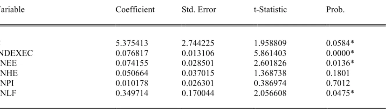
Table 3.3. Long run Estimation Dependent Variable: LNRGDP
Method: Least-Squares Sample: 1974/75-2014/15 Included Observation: 40
Variable Coefficient Std. Error t-Statistic Prob.
C 5.375413 2.744225 1.958809 0.0584* INDEXEC 0.076817 0.013106 5.861403 0.0000* LNEE 0.074155 0.028501 2.601826 0.0136* LNHE 0.050664 0.037015 1.368738 0.1801 LNPI 0.010178 0.026301 0.386974 0.7012 LNLF 0.349714 0.170044 2.056608 0.0475*
Source: - Own computation using EVIEWS 8. Note: - * indicates level of significance at 5%.
R2=0.984 F-Stat=418.2986 Prob (F-Stat)=0.0000 D.W. Stat=0.6684
Table 3.3, provides the long run relationship between variables. The coefficients of INDEXEC, LNEE, LNHE, LNPI, and LNLF appears with the expected sign and statistically significant at 5% level except LNHE and LNPI.
The result suggests that a one unit increase in economic infrastructure stock leads to an increase in real GDP by 0.076 percent and statistically significant. The intuition behind this result is that, extensive and efficient infrastructure is critical for ensuring the effective functioning of the economy as it is an important factor determining the location of economic activity and the kinds of activities or sectors that can develop in the domestic economy. Well-developed infrastructure reduces the effect of distance between regions, integrating the national market and connecting it at low cost to markets in other countries and regions. In addition, the quality and extensiveness of infrastructure networks significantly impact economic growth. A well-developed transport, communications, and energy infrastructure stock is thus a prerequisite for the access of less-developed communities to core economic activities and services in the country.
On the other hand the relationship with education sector development unveil that a one percent increase in education expenditure leads real GDP to increase by 0.074 percent and statistically significant. The result tells us knowledge and skills development also be key considerations of public sector infrastructure policies in Ethiopia, such policies are often justified in public expenditure in education. In terms of the theoretical model, skills acquisition constitutes an increase in the stock of human capital, so such acquisition may in fact have positively impact on economic growth.
Another social service sector examined in this study is expenditure pertinent to health sector development. A one percent increase in health expenditure leads real GDP to increase by 0.050 percent, but it’s not statistically significant. As a matter of fact, health affects economic growth directly through labor productivity and the economic burden of illnesses. Health also indirectly impacts economic growth since aspects such as child health affect the future income of people through the impact health has on education. This indirect impact is easier to understand if it is observed on a family level. When a family is healthy, both the mother and the father can hold a job, earn money which allows them to feed, protect and send their children to school. Healthy and well-nourished children will perform better in school and a better performance in school will positively impact their future income.
Ample empirical findings support this positive linkage between health status and economic growth. For instance in Britain, the combined impact of improved diets, reductions in infectious disease, better living standards, and environmental health resulted in increased labor force participation by poor, and increased output (Fogel, 2002). Similarly, East Asian countries experience shows, health improvements are identified as a major pillar of ‘economic miracle’, accounting for 1/3 of economic growth (Bloom and Canning, 2000).
As opposed to the above argument, some authors debate an expanding economy can co-exist with problems of income inequality and poverty. They point out that economic growth does not always lead to improvements in health and, conversely, improvements in health are not necessarily dependent on economic growth. They maintain that some countries (example, Brazil) have managed to receive impressive gains in reducing infant mortality rate during a period of just 1% growth in GDP per capita per year. (Ruhm, 2006) has argued that the
empirical evidences supporting the view of positive relationship between health status and economic growth are quite weak and come from studies containing methodological shortcomings that are difficult to remedy. Thus, the reason why expenditure on health results insignificant may be due to the proxy used in the study, it might results significant relationship if we use life expectancy or mortality rate.
The relationship real GDP has with private investment also results insignificant, a one percent increase in private investment leads to an increase in real GDP by 0.010 percent for the period under investigation.
This study examined the role of labour force; a one percent increase in labor force leads the real GDP to increase by 0.349 percent and statistically significant. This relationship is expected as working age population would help the economy to grow in both the exogenous and endogenous growth models.
Following the long run estimation using OLS method, the long run coefficients are estimated using ARDL model. The following table provides the long run relationship between the dependent and independent variables over the period under investigation. As in conventional cointegration testing, we're testing for the absence of a long-run equilibrium relationship between the variables. This absence coincides with zero long run coefficients for equation (2.6). A rejection of H0 implies that we have a long-run relationship.
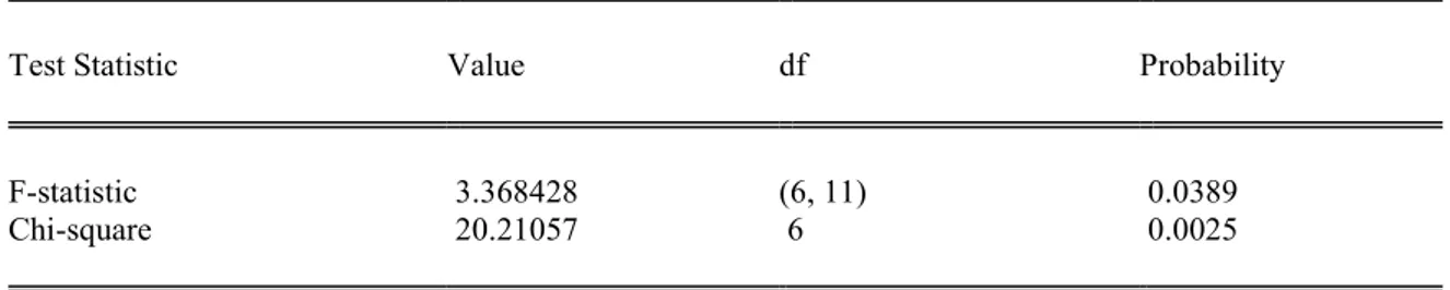
3.3.1. Bounds Test
The ARDL approach test for long run relationship between variables is conducted using bounds test method, and the computed F-statistics is identified. The Pesaran et.al (2001) table provides the upper and lower bound for the computed F stat, which is with in [2.476, 3.546] at 95% confidence interval.
Exact critical values for the F-test aren't available for an arbitrary mix of I(0) and I(1) variables. However, Pesaran et al. (2001) supply bounds on the critical values for the asymptotic distribution of the F-statistic. For various situations (example, different numbers of variables, (k + 1)), they give lower and upper bounds on the critical values. In each case, the lower bound is based on the assumption that all of the variables are I(0), and the upper bound is based on the assumption that all of the variables are I(1). The following table provides the bounds test result shown using Wald test.
If the computed F-statistic falls below the lower bound we would conclude that the variables are I(0), so no cointegration is possible, by definition. If the F-statistic exceeds the upper bound, we conclude that we have cointegration. Finally, if the F-statistic falls between the bounds, the test is inconclusive. Thus using the following table we can decide whether there is an evidence of a long run relationship between variables.
Table 3.4 Wald Test1
Source: - Own computation using EVIEWS 8.
From table 3.4, we can see that the F-statistics is 3.3684 which is within the range of [2.476, 3.546], that makes the long run relationship inconclusive or unsettled between variables. Therefore, we don’t have evidence to say the variables move together in the long run.
3.4. Short Run Relationship: ECM
The term error-correction relates to the fact that last-periods deviation from a long-run equilibrium, the error, influences its short-run dynamics. Thus ECMs directly estimate the speed at which a dependent variable returns to equilibrium after a change in other variables.
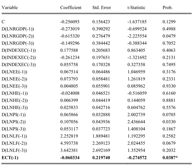
Accordingly, using the ARDL frame work after generating the ECT we can estimate the ECM. The optimal lag length is selected based on the information criterion (AIC, SIC, and HQ criterion). Thus, in order to determine the short run dynamics between variables the same lag order is used as ARDL model. The following table provides the ECM at lag 3.
The model estimates the short run coefficients of variable. An important term we generate to capture the short run dynamics of the system is the ECT, which measures the disequilibrium corrected each year if shock happens to the model. The speed of adjustment or the error correction term (ECT) in the model is represented by ECT (-1) and come up with the expected sign and level of significance. In an empirical sense, it implies 6% of
1 Recall, Null Hypothesis: C(2)=C(3)=C(4)=C(5)=C(6)=C(7)=0, which are the coefficients for LNRGDP(-1), INDEXEC(-1), LNEE(-1),
LNHE(-1), LNPI(-1), LNLF(-1).
Test Statistic Value df Probability
F-statistic 3.368428 (6, 11) 0.0389
the disturbance in the short run is corrected each year or the system is getting adjusted towards long run equilibrium at the speed of 6% annually.
Vis-à-vis about the model, the coefficient of determination (R2), indicates 64% of real GDP is explained by the variables included in the regression. Moreover, the overall significance of (F-test) established all variables are jointly significant.
Table 3.5 Results of ECM Dependent Variable: D (LNRGDP)
Method: Least Squares Sample (adjusted): 1984-2014 Included Observation: 31 observation
Variable Coefficient Std. Error t-Statistic Prob.
C -0.256093 0.156423 -1.637185 0.1299 D(LNRGDP(-1)) -0.273019 0.390292 -0.699524 0.4988 D(LNRGDP(-2)) -0.615320 0.276479 -2.225554 0.0479 D(LNRGDP(-3)) -0.149296 0.384442 -0.388344 0.7052 D(INDEXEC(-1)) 0.177588 0.205683 0.863405 0.4063 D(INDEXEC(-2)) -0.261234 0.197651 -1.321692 0.2131 D(INDEXEC(-3)) 0.055758 0.170328 0.327358 0.7495 D(LNEE(-1)) 0.067514 0.064486 1.046959 0.3176 D(LNEE(-2)) 0.073793 0.058481 1.261819 0.2331 D(LNEE(-3)) 0.004805 0.055901 0.085962 0.9330 D(LNHE(-1)) -0.024008 0.046521 -0.516059 0.6160 D(LNHE(-2)) 0.006399 0.044419 0.144059 0.8881 D(LNHE(-3)) 0.025833 0.042716 0.604762 0.5576 D(LNPI(-1)) 0.065866 0.032888 2.002739 0.0705 D(LNPI(-2)) 0.107056 0.043936 2.436644 0.0330 D(LNPI(-3)) 0.053117 0.037723 1.408104 0.1867 D(LNLF(-1)) 2.252819 1.889481 1.192295 0.2582 D(LNLF(-2)) 4.593738 2.269123 2.024455 0.0679 D(LNLF(-3)) 3.642381 2.692169 1.352954 0.2032 ECT(-1) -0.060334 0.219740 -0.274572 0.0387*
Source: - Own computation using EVIEWS 8. Note: - * Imply level of significance at 5%.
R2=0.6460 F-Stat=1.0565 Prob (F-Stat) =0.4790 D.W. Stat=1.8327 4. CONCLUSION AND RECOMMENDATION
This research challenges a belief that, there is relationship infrastructure development has with economic growth in the long run as well as short run. To this end, time series data is used from 1974/75-2014/15, a period spanning 40 years. The econometric analysis starts from identifying the time series nature of variables, identifying the correct lag length and proceed with the long run and short run analysis. ARDL bounds test, and ECM has been used to infer the long run relationship and short run dynamics within variables.
The long run dynamics using cointegration procedure allows us to specify the dynamic adjustment among the cointegrated variables. The bounds test confirms there is no evidence for the existence of long run relationship; i.e., all the variables moving together in the long run. However, estimation using OLS provides economic growth has a positive relationship with economic infrastructure stock (INDEXEC), education expenditure (LNEE), health expenditure (LNHE), private investment (LNPI), and labor force (LNLF) even though statistical significance is not supported by (LNHE, LNPI). The notation we derive from such kind of relationship is infrastructure development is crucial for economic growth in Ethiopia over the periods under investigation.
The short run dynamics is estimated using the error correction mechanisms. The model came up with the expected sign and level of significance. The negative sign affirms the whole system get adjusted towards the long run equilibrium. Based on the above findings the study forward some policy issues that should be considered in order to strengthen the relationship between infrastructure development and economic growth in Ethiopia.
Given a positive impact from economic and social service infrastructure development on economic growth, health sector and private investment development doesn’t play significant role on economic growth for the period under investigation. Hence, it would be more effective if government give due attention on the quality aspect of the health sector development and also government huge intervention in the economy crowds in private investment role in the economy. It is therefore, useful for the government to reduce its huge intervention in the economy.
In the long run there is no evidence regarding the movement of variables together. Its implication is that policy issues are not designed concurrently with economic growth to address the infrastructure gap the country faces.1 Thus, it would be very helpful for an efficient and effective implementation of economic growth policies, the provision of developed infrastructure facilities in advance.
In the short run the role of infrastructure to adjust short run disequilibrium is too small. It shows us if shock happens to the economy its role to bring the shock back to long run growth path is minimal. Therefore, mechanisms should developed to galvanize its role either private-public partnership or creating conducive private investment environments at policy level.
There are several ways to extend this paper. Since the impact infrastructure and economic growth is the center of debate, it could be possible to extend the debate for Ethiopia by examining the correlation side, using social sector infrastructure index, and some more quality measure indicators.
References
Abramowitz, M. 1956. “Resource and Output Trends in the United States since 1870”. American Economic Review 46 (May): 5-23.
Admasu Shiferaw, Eyerusalem Siba, Getnet Alemu, Mans Soderbom, (2013), “Road Infrastructure and enterprise Dynamics in Ethiopia”, Unpublished Thesis, The College of William and Mary, USA.
Admit, Haile & James, 2014, Ethiopia, African economic outlook, Various Issues, pp.15.
Arrow, K., and M. Kurz (1970), Public Investment: The Rate of Return and Optimal Fiscal Policy, Johns Hopkins.
Barro RJ (1990) Government spending in a simple model of endogenous growth. J Polit Econ 98 (5):103–125. Barro, R. (1991), “Economic Growth in a Cross Section of Countries,” Quarterly Journal of Economics, 106,
407-443.
Bloom, D. E. and D. Canning. (2000), “The Health and Wealth of Nations.” Science 287: 1207–8.
Boopen Seetanah, the economic importance of education: evidence from Africa using dynamic panel data analysis, Journal of Applied Economics, Vol. 12, no. 1, pp. 137-157.
Butkiewicz, JL & Yanikkaya, H 2005, 'The effects of IMF and World Bank lending on long-run economic growth: an empirical analysis', World Development, vol. 33, no. 3, pp. 371-391.
Christopher Ruhm, Deaths rise in good economic times: Evidence from the OECD, Economics & Human Biology, 2006, vol. 4, issue 3, pages 298-316
Colombage, SRN 2009, ‘Financial markets and economic performances: Empirical evidence from five industrialized economies’, Research in International Business and Finance, vol. 23, no. 3, pp. 339-348. Devarajan, Swaroop, and Heng-fu Zou (1996), The Composition of Public Expenditure and Economic Growth,
Journal of Monetary Economics, 37, pp.313-44.
Engle, RF, Newbold, P & Granger, CWJ, 1995, 'Co-integration and error correction: representation, estimation and testing', Econometrica, vol. 55, no. 2, pp. 251-276.
Fogel, R. W. (1994), “Economic Growth, Population Theory, and Physiology: The Bearing of Long Term Process on the Making of Economic Policy”. American Economic Review 84 (3): 369–395.
Gary Fogel, Evolutionary computation in bioinformatics, 2002, Morgan Kautmann Publisher. Gujarati, D.N, 2004, Basic Econometrics, 4th ed. McGraw-Hill Companies.
Hahn, FR 2008, 'the finance-specialization-growth nexus: evidence from OECD countries', Applied Financial Economics, vol. 18, no. 4, pp. 255-265.
IMF, Annual Report of the Executive Board, From Stabilization to Sustainable Growth, 2014.
Karran, T 1985. The determinants of taxation in Britain: an empirical test, Journal of Public Policy, vol. 5, no. 3, pp. 365-386.
Koch, S, Schoeman, N & Tonder, J 2005, ‘Economic growth and the structure of taxes in South Africa: 1960–
2002', The South African Journal of Economics, vol. 73, no. 2, pp. 190-210.
Lucas, R. (1988), “On the Mechanics of Economic Development,” Journal of Monetary Economics, 22, 3-42. Oyesiku Kayode, Onakoya, Adegbemi Babatunde, Folawewo Abiodun. An Empirical Analysis of Transport
Infrastructure Investment and Economic Growth in Nigeria. Social Sciences. Vol. 2, No. 6, 2013, pp. 179-188. doi: 10.11648/j.ss.20130206.12.
Pesaran, M.H. and B. Pesaran, 1997. Working with microfit 4.0: Interactive econometric analysis. Oxford: Oxford University Press.
Pesaran, M.H., Y. Shin and R.J. Smith, 2001. Bounds testing approaches to the analysis of level relationships. Journal of Applied Econometrics, 16(3): 289-326.
Pravakar S, Ranjan.K. D, Geethanjali N, (2012), Chia’s Growth Story: The Role of Physical and Social Infrastructure, Journal of Economic Development, Volume 37, Number 1.
Robert M. Solow, Technical Change and the Aggregate Production Function, The Review of Economics and Statistics, Vol. 39, No. 3 (Aug., 1957), pp. 312-320.
Robert. J. Barro, Xavier Sala-Martin, The Journal of Political Economy, 1992, Vol. 100, no. 2, pp. 223-251. Romp W, de Haan J (2005) Public capital and economic growth: A critical survey, EIB papers 10 (1). European
Investment Bank, Luxemburg.
Soli, VO, Harvey, SK & Hagan, E 2008, ‘Fiscal policy, private investment and economic growth: the case of Ghana', Studies in Economics and Finance, vol. 25, no. 2, pp. 112-130.
Teklebirhan Alemnew, (2015), “Public Infrastructure Investment, Private Investment and Economic Growth in Ethiopia: Co-Integrated VAR Approach”, Unpublished MSc Thesis, Addis Ababa University, Addis Ababa, Ethiopia.
Tofik S. 2012, “Official Development Assistance (ODA), Public Spending and Economic Growth in Ethiopia”, Journal of Economics and International Finance, vol.4 (8), pp.173-191.
Tsoukis C, Miller NJ (2003) Public services and endogenous growth. J Policy Model 25.
Yang, W. Z.; Beauchemin, K. A; Rode, L. M., 2001. Barley processing, forage: concentrate, and forage length effects on chewing and digesta passage in lactating cows. J. Dairy Sci., 84: 2709-2720
Yetnayet Ayalneh, (2012), “Evaluating Transport Network Structure: Case Study in Addis Ababa, Ethiopia”, Unpublished MSc Thesis, University of Twente, the Netherlands.