SPE 163585
A New Approach to Load Balance for Parallel Compositional Simulation
Based on Reservoir Model Over-decomposition
Yuhe Wang, SPE, John E. Killough, SPE, Texas A&M University
Copyright 2013, Society of Petroleum Engineers
This paper was prepared for presentation at the SPE Reservoir Simulation Symposium held in The Woodlands, Texas USA, 18–20 February 2013.
This paper was selected for presentation by an SPE program committee following review of information contained in an abstract submitted by the author(s). Contents of the paper have not been reviewed by the Society of Petroleum Engineers and are subject to correction by the author(s). The material does not necessarily reflect any position of the Society of Petroleum Engineers, its officers, or members. Electronic reproduction, distribution, or storage of any part of this paper without the written consent of the Society of Petroleum Engineers is prohibited. Permission to reproduce in print is restricted to an abstract of not more than 300 words; illustrations may not be copied. The abstract must contain conspicuous acknowledgment of SPE copyright.
Abstract
The quest for efficient and scalable parallel reservoir simulators has been evolving with the advancement of high performance computing architectures. Among the various challenges of efficiency and scalability, load imbalance is a major obstacle that has not been fully addressed and solved. The reasons that cause load imbalance in parallel reservoir simulation are both static and dynamic. Robust graph partitioning algorithms are capable of handling static load imbalance by decomposing the underlying reservoir geometry to distribute a roughly equal load to each processor. However, these loads determined by a static load balancer seldom remain unchanged as the simulation proceeds in time. This so called dynamic imbalance can be further exacerbated in parallel compositional simulations. The flash calculations for equations of state in complex compositional simulations not only can consume over half of the total execution time but also are difficult to balance merely by a static load balancer. The computational cost of flash calculations in each grid block heavily depends on the dynamic data such as pressure, temperature, and hydrocarbon composition. Thus, any static assignment of grid blocks may lead to dynamic load imbalance in unpredictable manners. A dynamic load balancer can often provide solutions for this difficulty. However, traditional techniques are inflexible and tedious to implement in legacy reservoir simulators. In this paper, we present a new approach to address dynamic load imbalance in parallel compositional simulation. It over-decomposes the reservoir model to assign each processor a bundle of subdomains. Processors treat these bundles of subdomains as virtual processes or user-level migratable threads which can be dynamically migrated across processors in the run-time system. This technique is shown to be capable of achieving better overlap between computation and communication for cache efficiency. We employ this approach in a legacy reservoir simulator and demonstrate reduction in the execution time of parallel compositional simulations while requiring minimal changes to the source code. Finally, it is shown that domain over-decomposition together with a load balancer can improve speedup from 29.27 to 62.38 on 64 physical processors for a realistic simulation problem.
Introduction
High performance computing including parallel computing plays a vital role in many areas of engineering, such as defense, energy and financial engineering. Nowadays, these devices are being widely used by domain application engineers and scientists to solve a variety of commercially and scientifically interesting computationally intensive problems. Many of the techniques utilized are associated with solving the discretized partial differential equations that describe the underlying physics. Reservoir simulation, which mimics or infers the behavior of fluid flow in a petroleum reservoir system through the use of mathematical models, is one of the methods that is widely used in petroleum upstream development and production. Reservoir simulator was born as an efficient tool for reservoir engineers to better understand and manage assets. However, like any numerical simulation tool, reservoir simulation is inherently computationally intensive and easily becomes inefficient if larger and larger grids or more components are necessary to describe accurately the complex phenomena occurring in the subsurface of the earth. Therefore, execution of reservoir simulation on parallel computers seems be the apparently feasible way to tackle the computational demand of reservoir simulation. Although running reservoir simulation in parallel sounds extremely attractive, developing an efficient parallel reservoir simulator is far more challenging than developing the underlying serial reservoir simulator. For decades there have remained many open problems associated with high performance computing and reservoir simulation.
The quest for efficient and scalable parallel reservoir simulators has been evolving with the advancement of high performance computing architectures. The mainframes of decades ago quickly gave way to workstations, clusters, and finally
PCs as technology advanced and costs were dramatically reduced. Each of these evolutionary steps led to significant changes in reservoir simulators. The era of serial reservoir simulation was replaced by vectorized and finally parallelized simulation. An elusive goal of reservoir simulation has been the ability to efficiently utilize massively parallel processing.
In the past the majority of effort has been spent on developing robust parallel linear solvers (Killough and Wheeler 1987; Cao et al. 2005; Fung and Dogru 2007). As Graphic Processing Units (GPUs) have become more and more popular in the oil industry (Foltinek et al. 2009; Appleyard et al. 2011; Klie et al. 2011; Liu et al. 2012; Bayat and Killough, 2013), it is expected that the reservoir simulation community will soon have a GPU accelerated linear solver commercially implemented for reservoir simulation.
Massively parallel linear solver development has by no means been completed; however, little effort has been spent on investigating another important aspect of high performance simulation - load balancing. Load imbalance has become a major obstacle for parallel performance. The reasons that cause load imbalance in parallel reservoir simulation are both static and dynamic. Robust graph partitioning algorithms are capable of handling static load imbalance by decomposing the underlying reservoir geometry to distribute roughly equal load to each processor. This approach works well to distribute the load for parallel linear solver. Metis from the University of Minnesota is one of most popular tool for graph partitioning (Karypis and Kumar 1999) and has been applied in parallel linear solver packages and parallel reservoir simulation both commercially and academically (Shuttleworth et al. 2009; Zhang et al. 2001). In black oil simulation, where the linear solver can often take over 90% of the total execution time, graph partitioning can often cure the load imbalance problem. However, this is not the case for compositional reservoir simulation. In fully compositional simulation, the time spent on equation of state computations can be more than 70% of the total computational time. Although the underlying grid is divided equally (roughly) to each processor, the loads determined by a static load balancer such as Metis seldom remain unchanged for fully compositional simulation, especially for the equation of state computations. The changing of load as simulation running - the so-called dynamic load imbalance - is difficult to balance merely by a static load balancer. The reason for this is that each of the underlying grid blocks has an independent phase behavior calculation. The computational cost of the associated flash calculations in each grid block heavily depends on the dynamic data such as pressure, temperature, and fluid composition. It is well known that flash calculations can vary tremendously with time in each grid block. The cost can become very high when phase changes happen in a grid block or when the fluid mixture is near the critical point. Since the conditions that cause expensive flash calculations are difficult to predict a priori, any static assignment of grid blocks may lead to dynamic load imbalance in unpredictable manners. Removing this load imbalance in compositional reservoir simulation remains mostly an open problem. A dynamic load balancer is clearly needed to alleviate this difficulty.
Sherman (1992) proposed a dynamic load-balancing scheme for parallel compositional simulation base on Linda coordination language. However, this parallel programming model is not widely used as opposed to MPI (Massage Passing Interface). Killough and Anguille et al. (1995) developed an improved load-sharing and receiver-initiated dynamic load balancing algorithm for parallel compositional simulation and reported substantial improvement. Little or no research has been reported over the past decade in this area. In essence, to optimize the parallel performance by communicating information from one processor to another relies on message passing. The overhead, or the time involved in message passing creates extra elapsed time which is added to the total computational time. Thus, in principle, all load-balancing schemes can be treated as a compromise between the reduction of load imbalance and minimization of the overhead. However, this improvement is likely to degrade with more processors since this mechanism requires a significant amount of data exchange between processors. As a model is scaled to more processors, this overhead may offset any potential gain by a load-balancing scheme. Moreover, implementing dynamic load balancing requires intimate knowledge of the underlying reservoir simulator source code. It can be quite tricky and cumbersome to determine which variables must be exchanged between processors for legacy comprehensive reservoir simulators.
In this paper, we present a novel approach to address the dynamic load imbalance issue in parallel compositional simulation. This new methodology over-decomposes the underlying reservoir model into mini-subdomains. Based on the Charm++ infrastructure, a bundle of mini-subdomains are assigned to the available physical processors. Processors treat these bundles of mini-subdomains as virtual processes or user-level migratable threads, which can be dynamically migrated across processors in the runtime system. To our best knowledge, this is the first adaptation of domain over-decomposition or processor virtualization to reservoir simulation.
Our approach can seamlessly handle static and dynamic load imbalance in a uniform fashion. Further more, this new approach requires minimal changes to the original MPI based reservoir simulator. The main contribution of this paper is to demonstrate that domain over-decomposition implemented as virtual processes can be applied to improve parallel performance of MPI based compositional reservoir simulations that suffer from load imbalance issues. The rest of the paper is organized as follows. We first present the legacy comprehensive reservoir simulator used in this study and the main features of Charm++. Next, we describe the parallelization of equation of state calculation using MPI and how we adapted it to exploit processor virtualization followed by results from our experiments. Conclusions and outlooks are provided at last. Background
1. A Commercial Comprehensive Reservoir Simulator
A commercial comprehensive reservoir simulator (simulator hereafter) written by Fortran 90 and C is applied as the test bed in this study (Dean and Lo, 1988). Based on fully implicit and IMPES formulations, the simulator is capable of performing
black oil, limited compositional and fully compositional simulation for single and dual porosity reservoirs. It utilizes 3D radial and corner point grid system and supports multiple levels of local grid refinements. Wellbore parameters are treated implicitly during the simulation process and wells can be connected into surface networks. Geomechanics is also supported. Stress, strains, and displacements can be calculated throughout the simulation in a fully coupled fashion with flow calculations. The linearized equation system is solved by iterative solvers with preconditioning and acceleration options. In a word, this is a comprehensive reservoir simulator with production quality. The hope is to demonstrate that the technique introduced below is applicable to real-strength reservoir simulators.
2. Charm++ and Processor Virtualization
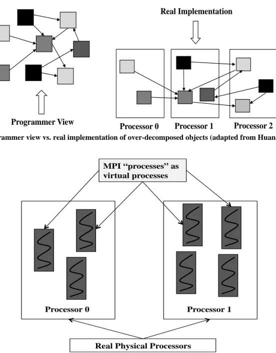
Charm++ (Kale et al. 2008) is an objective-oriented parallel programming library for C++/C/Fortran. It aims to improve productivity in parallel code development and enhance parallel scalability. Charm++ is message-driven. It does not block the processors while waiting for messages to be received. Based on migratable objects, Charm++ uses the idea of processor virtualization. In this framework, the programmer decomposes a domain into N subdomains to execute on P processors. In ideal case, we should have N >> P. In the programmer’s point of view, it is seen that the program is running using N subdomains. The Charm++ runtime system maps those subdomains or more specifically Charm++ objects to the P available processors. Fig. 1 provides a schematic illustration of the basic idea of processor virtualization. The ratio of N over P is the so called processor virtualization ratio. The mapping is dynamic and the subdomains can migrate across processors during program running. This unique capability is utilized by the underlying intelligent Charm++ runtime system, which provides potential for better overlapping between computation and communication and cache utilization.
The combination of a natural encapsulation mechanism and an intelligent runtime system has made Charm++ suitable for parallel code development over a range of computing architectures, from personal computers to large-scale parallel clusters, from multicore CPUs to massively-parallel GPUs. In addition, it has been applied to scale real-world applications to thousands of processors on several scientific and engineering fields, such as quantum chemistry (Bohm et al. 2008), computational cosmology (Jetley et al. 2008), rocket simulation (Jiao et al. 2005) and weather forecasting (Rodrigues et al. 2010, 2011).
3. Adaptive MPI
Adaptive MPI (AMPI) is an implementation of the MPI standard on top of Charm++ (Huang et al. 2003, 2006; Zheng et al. 2006). As abovementioned, the developer only sees the virtual processors while the mapping of virtual processors to physical processors is handled by the Charm++ runtime system. It is illustrated in Fig. 2 that in AMPI the original MPI processes from a programmer’s perspective are embedded in a Charm++ object as user-level threads. These user-level threads are not only migratable between physical processors but also have very short context switch times. In the context of AMPI, the N MPI tasks in a MPI code are referred as Virtual Processors (VPs). A VP is assigned as a user level thread and a bundle of VPs share one physical processor. Without any programming effort, the overlap between computation and communication is automatically achieved by having more VPs than real physical processors. When one VP is blocked from communication, the Charm++ scheduler picks up the next VP to execute. More specifically, when some VPs of a physical processor are waiting for messages to be received, other VPs can continue their execution in this particular physical processor. Since smaller subdomains may fit into cache if the over-decomposition is enough, better cache utilization is expected in this situation. Therefore, it is natural to see legacy MPI code will benefit substantially from AMPI and this potentially significant benefit comes with few catches and without major modifications of the original MPI code.
However, to utilize AMPI in practice, one must pay attention to global and static variables. Those variables are problematic for a multi-threaded programming model such as OpenMP and AMPI. In MPI, since only one thread exists in the allocated process’s address space, global and static variables are safe. But, if a single instance of a global or static variables is shared by more than one thread in the single address space, incorrect results are likely to be generated. In other words, VPs residing on a particular physical processor will access the same copy of global and static variables. If those variables are to be read and updated, conflicts will occur and correct results cannot be guaranteed. Thus, one has to privatize global and static variables. There are a few approaches for this privatization which will be discussed in following sections.
4. Native Load Balancing in AMPI and Charm++
Charm++ provides a native and powerful infrastructure for load balancing. Charm++ is based on the idea that load behaviors from the recent past provide sound predication for loads in the near future. By actually measuring the load information at runtime, it migrates VPs from heavily loaded processors to lightly loaded processors. Thus, Charm++ can be treated as a measurement-based load balancing technique. Several different load balancing policies have been made available by Zheng (2005). In addition, a new load balancer can be written simply by using the Charm++ API. The different load balancing schemes are selected in the command line at execution time.
The specific subroutine to invoke the load balancer in AMPI is MPI_Migrate(). When MPI_Migrate() is called, VPs may migrate between processors, if it is determined that such migration will improve parallel performance. Obviously, the frequency of calling MPI_Migrate() is determined by the compromise between the overhead and performance degradation caused by load imbalance.
5. Ideal Load Balancing Model
An ideal load balancing model can be stated as an optimization problem. We proposed an objective function to optimize the load of M threads among N processors based on (Rodrigues et al. 2010). The objective function f is as follows, which belongs to mixed integer quadratic programming.
1 0 1 0 1 1 1 0 2 1 0 N i N k N k l N k kb ka lb ka mean M j ij jx
L
Cx
x
Sx
x
f
is the weight of VP j and
L
meanis the average load. is a binary which represents the placement of VP j on processor i.
is the weight of communication cost.C
represents the inter-processor communication cost whileS
is the communication for VPs that reside in the same processor. This objective function penalizes both computational and communication cost. Even with the fastest machine and solver, solving this mixed integer quadratic programming problem for modest number of VPs and processors for optimality can take an excessive amount of time. Hence, a heuristic approach must be used to deal with realistic applications. Some of the heuristic approaches will be discussed in next section.Adaptation of Reservoir Simulator to AMPI
Generally speaking, adapting an MPI program to AMPI is a simple process. But as explained in the previous section, one must pay attention to the global and static variables. Since the original simulator is serial, the first required step is to parallelize a portion or all of the simulator using MPI. In this section, we present the parallelization of the equation of state of simulator, possible ways of global and static variables privatization, and different load balancing schemes.
1. Equation of State Parallelization
To serve as a proof of concept study, in this paper we only parallelize the equation of state computations which can take more than 70% of the total execution time. The idea of parallelization of this portion of the compositional simulator is rather straightforward. Since the flash calculations for each grid block are independent from other grid blocks, no subdomain boundary data exchange is needed. Basically, at the equation of state subroutine, we do the follow four steps:
1. Divide the key input and output arrays according to the domain decomposition setup. We use 2-D domain decomposition, i.e. the reservoir is divided in X and Y directions while keeping the Z direction undivided. This domain decomposition setting is reasonable since in general the Z direction extent is far less than the X and Y directions.
2. Let the master processor distribute necessary information to the slave processors. 3. Each processor performs equation of state computations independently.
4. Let the master processor gather computed information from the slave processors. Once the master has finish gathering, all processors then exit the equation of state subroutine.
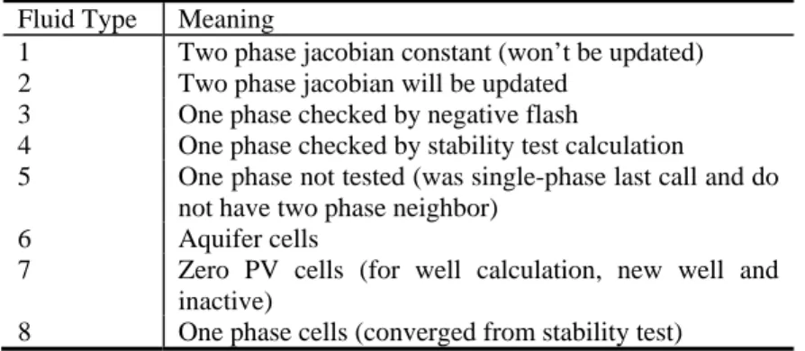
Although it seems to be an easy parallelization according to the above four steps, it is not the case for a comprehensive reservoir simulator. The equation of state and other involved code in this parallelization is about 20K lines. Moreover, the grid blocks are reordered inside flash calculation according to their fluid types. Table 1 lists the eight fluid types. Thus, we
Table 1 – Fluid types in the flash calculation Fluid Type Meaning
1 Two phase jacobian constant (won’t be updated) 2 Two phase jacobian will be updated
3 One phase checked by negative flash
4 One phase checked by stability test calculation
5 One phase not tested (was single-phase last call and do not have two phase neighbor)
6 Aquifer cells
7 Zero PV cells (for well calculation, new well and inactive)
8 One phase cells (converged from stability test)
could not expect a big DO loop over all grid blocks, which can be parallelized easily as shown in Table 2. N is the total number of grid blocks that are to be flashed. numproc is the number of requested processors. So, N_local is the number of
j
grid blocks that are assigned to each available processor. Note that, to shorten the presentation, it is assumed that N can be divided by numproc exactly. A and A_local represent the arrays which are to be updated by flash calculations. A_local is allocated to each available processor to store information computed. A is the global array to collect information from each available processor. To be concise yet complete, we omit the actually arguments of MPI and subroutine calls. As abovementioned, since the grid blocks are reordered according to fluid types, we construct and parallelize a derived type on top of the actual equation of state routine to govern the data structure in the flash calculations. In the derived type, pointers are set up to trace the grid blocks to be updated in each subdomain. In this setting, we do not need to worry about the grid reordering inside of the flash calculation.
Table 2 – Pseudo Fortran MPI code for flash calculation N_local = N/numproc
! Broadcast variables and arrays to slave processors CALL MPI_BCAST()
DO i = 1,N_local A_local(i) = flash() ENDDO
IF (myid == Master) THEN
! put A_local computed by master to global A A = A_local
DO i = 1,numproc-1 CALL MPI_RECV()
! put A_local computed by slaves to global A A = A_local
ENDDO
ELSEIF (myid /= 0) THEN CALL MPI_SEND() ENDIF
Since we only parallelize a portion of the simulator, we let the master processor perform the rest of the simulation. Special care must be paid to places where GOTO statements are used such as when the newton iteration is not converged and time step reduction is performed. Otherwise, a deadlock condition will be likely occurring. Table 3 lists a situation in which a deadlock might happen. No deadlock will happen if label 1000 is inside the IF_Master structure. However, when label 1000 is outside of IF_Master and slave processors need to perform computation after this label, deadlock will happen if trigger is true. This is because only the master processor gets the signal to go to label 1000 while other slave processors are hanging there. If this situation happens, the program will be waiting with slave processors at label 1000 and the program will stall. Since there is no OMP Flush like function in MPI to flush all the processes to have the same view of a variable, to fix this issue we should broadcast the triggers to all the processors and let all processors go to label 1000 explicitly. A quick fix for Table 3 is provided in Table 4.
Table 3 – Pseudo Fortran code that may cause deadlock IF_Master : IF (myid == Master) THEN
Perform computation
IF (trigger == .TURE.) THEN GOTO 1000
ENDIF
ENDIF IF_Master
Table 4 – Pseudo Fortran code to fix deadlock IF_Master : IF (myid == Master) THEN
Perform computation ENDIF IF_Master
CALL MPI_BCAST(trigger) IF (trigger == .TURE.) THEN GOTO 1000
ENDIF
It is readily seen that the slowest processor determines the time spent in equation of state. If one or few processors contain grid blocks that have phase changes or are at critical condition, those busy processors will dominate the computation time while other processors are idle. It is difficult to predict which processor will be busy. One may argue that a processor which has wells, will be busy; but such processors will not always be the busiest due to the processes occurring around the moving
injectant-displacement front. This front movement is generally unknown a priori (since predicting where the front will go and how long it will take is what the simulator is designed for). One may also argue that we can estimate where the fluid will go roughly from the permeability field, but decomposing a real world reservoir according to the permeability will complicate the coding to an even greater extent. Moreover, even we could assign more processors to high permeability channels; this will not help since we still do not know when the front arrives at a certain place a priori. The only feasible and unified approach for this issue is to use finer grained computation and migrate those fine-grained units when necessary in a smart run-time system, which Charm++ can provide.
2. Domain Over-Decomposition
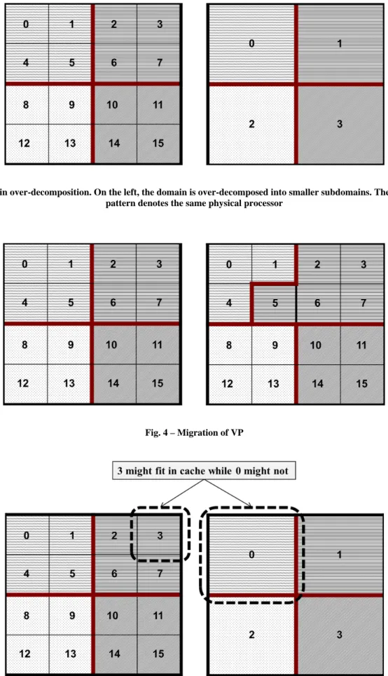
As explained in the previous section, processor virtualization is required to enhance parallel performance of an existing MPI code. It is not redundant to emphasize again that one can just decompose the domain as if as many as processors that are required are available. In other words, the MPI code does not need to be changed at all in this aspect. For example, as shown in Fig. 3, one just decomposes the domain as if there are 16 processors. But in fact, these are 16 VPs that are to be mapped to the 4 physical processors. In Fig. 3, the thick lines divide the physical processors while the thin lines separate the VPs. In this example, the processor virtualization ratio is 4. One should also appreciate that such over-decomposition may enhance cache utilization. As shown in Fig. 5, subdomain 3 might fit in cache while subdomain 0 might not. Note that over-decomposition is applicable if and only if the results are independent of the number of MPI tasks and one should be beware of the increase in memory usage due to over-decomposition.
3. Variable Privatization
As illustrated in Fig. 3, 4 VPs share one physical processor. We have discussed that such a scenario will cause problems if global and static variables are used. Thus, these variables have to be privatized. It is noted that, in Fortran, module variables, saved subroutine variables, and common blocks belong to this category. Fortunately, since we only execute the equation of state in parallel, the number of variables to be privatized is not significant. Table 5 lists the number of global, static variables and common blocks. Currently, there are 4 approaches to privatize global and static variables with different mechanisms and applicability:
Table 5 Number of variables to privatize Globals Static Commons
124 4 0 3.1 Manual Change
The thought behind manual change is to pass the information those global variables carry as subroutine arguments, since subroutine arguments are passed on a stack which are not shared across threads. We could gather global variables together in a single derived type in Fortran 90. This derived type is allocated by each thread dynamically. We then set up a pointer to this derived type. The pointer is passed across the subroutine as an argument. This mechanism will make sure each thread owns a private copy of the global variables. Static variables can be handled in the same way. As the name suggests, this privatization requires manual changes of all of these variables, which can be very tedious and bug-prone if the number of global variables is significant. Thus, it is clearly not a good approach for a large legacy reservoir simulator.
3.2 Source-to-source Transformation
There is a way to do the manual change automatically. A tool called Photran by Zheng et al. (2011) is available to transform the source code to change global and static variables in objects and then pass the objects across subroutines. Photran works by constructing abstract syntax trees of the program. However, at the time of preparation of this paper, Photran is only in beta phase. In our limited experiments, this tool works well for simple example code but is tends to be unstable or even crash for large code. Moreover, the readability of the transformed code by Photran decreases to some extent. Therefore, it is not recommended to apply Photran until a stable version is released.
3.3 Automatic Global Variables Swapping
AMPI provides a build-in compilation flag that can automatically privatize global variables on systems that support Executable and Linkable Format (ELF). ELF is now a standard for objective files in Unix-like systems. It works as it maintains a Global Offset Table (GOT) for global variables and switches GOT contents at thread context switching. It is very straightforward to apply this approach. All one need to do is to add the flag –swapglobals at compilation and link time, which will enforce that each VP has its own view of a certain global variable. It works for C/C++/Fortran and x86 and x86_64 platforms. However, the drawback is that it does not handle static variables and has a context switch overhead that grows with the number of global variables. For static variables, we could replace saved local variables with a module, which transforms static variables to global variables. Since in this study the number of global and static variables is not high, in this paper we apply this approach.
3.4 Privatization Based on Thread Local Storage (TLS)
It is easy to appreciate that when the number of global and static variables is significant, which is often the case for a comprehensive parallel reservoir simulator, the overhead caused at context switch by –swapglobals may become excessive. Thus, clearly automatic global variables swapping is not the silver bullet for a comprehensive parallel reservoir simulator. Rodrigues et al. (2010) developed a better privatization strategy based on TLS (Thread Local Storage). TLS is designed for thread safety. This approach works by allocating one instance of the variable per thread. To utilize TLS to privatize global and static variables, one just need to add C directive “__thread” before all global and static variables. This simple modification will make these variables have thread local storage duration, which means a unique instance of a particular global or static variable is created for each thread that uses it and is destroyed when the thread terminates in a multi-threaded environment. Privatization based on TLS not only has no context switch overhead but also can handle both global and static variables. However, unfortunately, only C/C++ compilers have implemented TLS at this time and there is no such directive in Fortran. As a workaround for Fortran program, one can write a GFortran patch file to modify GFortran to adopt the TLS method for global and static variables privatization. How to modify GFortran compiler is certainly beyond the scope of this paper. At the time when this paper was prepared, a patch file for GCC 4.5 is being developed for our future study based on (Rodrigues et al. 2010; Rodrigues 2012). This approach is recommended if one want to apply AMPI to a comprehensive parallel reservoir simulator written in Fortran.
In summary, although we apply automatic global variable swapping for variable privatization, the TLS based privatization might be the only applicable strategy for a comprehensive parallel reservoir simulator at this time. Even if one has to have a modified GFortran for Fortran MPI code, this obstacle is not significant to surmount if one can adsorb or find expertise on compiler writing. One must keep in mind that global variable swapping and TLS are not supported by all platforms. For example, Blue Gene/P and Mac OS X support neither of them and Cray/XT only supports TLS. In fact, only the first two methods are applicable for all platforms. Therefore, when a stable Photran is debuted, the adaptation of MPI code to AMPI might become truly trouble-free.
4. Dynamic load balancer
As stated previously, Charm++ and AMPI can migrate VPs across processors to balance load. As illustrated in Fig. 4, when Processor 0 becomes overloaded while Processor 1 is under loaded, VP 5 will be migrated to Processor 1 if a load balancer is invoked. To utilize the dynamic load balancing strategy of AMPI, one only need to insert MPI_Migrate() calls at a certain frequency and setup the dynamic load balancer at compilation and runtime in the command line. In the reservoir simulator we can call MPI_Migrate() every nt time steps as follows:
IF (mod(time_step, nt) == 0) CALL MPI_Migrate()
We adapt the methodology of Rodrigues et al. (2010) to quantify imbalance by how much the load in the most loaded processor is above the average load. An imbalance threshold can also be set to trigger migrations.
Charm++ provides several dynamic load balancers that consider computational and/or communication load. The selection of a specific load balancer depends on the application itself. If an application only has computational load and no communication traffic, a balancer that only takes computational load into account will be enough. Otherwise, a balancer based both on computational and communication loads must be chosen.
Since inter-subdomain data exchange is not necessary for equation of state computations, we may choose dynamic load balancers that only handle computational load. Two balancers are selected in this study: GreedyLB and RefineLB. GreedyLB uses a greedy algorithm to assign the heaviest object to the least loaded processor till a balance is reached. RefineLB not only moves objects from overloaded processors to under loaded ones but also limits the number of objects migrated. In general, RefineLB is useful when only a few VPs migrations are sufficient to reach balance.
Although the case application in this paper does not need ghost cells along subdomain boundaries to exchange data, it is worth mentioning the dynamic load balancers that also take communication traffic into consideration. This kind of balancer is required for a general parallel reservoir simulator. The following discussion will also serve as a reference for our future study. The build-in balancers in this perspective are GreedyCommLB, RefineCommLB, RecBisectBfLB and MetisLB. GreedyCommLB extends GreedyLB to take the communication graph into account. RefineCommLB applies the same idea as RefineLB but takes communication into account. RecBisectBfLB recursively partition the communication graph until the number of partitions is equal to the number of processors. However, RecBisecBfLB does not explicitly guarantee that communication traffic is minimized. MetisLB uses Metis to partition the communication graph. The selection of these balancers is application dependent and heuristic. A systematic comparison between these balancers is recommended to understand their behavior for a particular application. It is noted that none of these balancers explicitly consider the spatial relationship between VPs. Thus, neighboring VPs might be distributed to different processors or even far away nodes in runtime. This is clearly not an optimal scenario since there might be communication between neighboring VPs. Thus, a balancer that considering the spatial relationship between VPs is preferred. Rodrigues et al. (2010) developed a new balancer based on Hilbert curve to consider such situations.
Example
In this section, we provide a case study for applying the domain over-decomposition and dynamic load balancing techniques for parallel equation of states computation of compositional simulation. We begin with describing the compositional reservoir model used in this case study and showing results of MPI execution on 64 physical processors. Next, we study the effects of domain over-decomposition and load balancing on this case model. We first show the results of domain over-decomposition without load balancing by simply varying the processor virtualization ratio. We then bring the effect of load balancing by dynamically migrating VPs during simulation execution.
All the simulations are performed on an IBM iDataplex cluster with Intel 8-way Nehalem and 12-way Westmere processors. All the cores are at 2.8 GHz and nodes are connected via 4X QDR infiniband. The development tools used are Intel Fortran and C compilers and Open MPI.
1. Reservoir Model
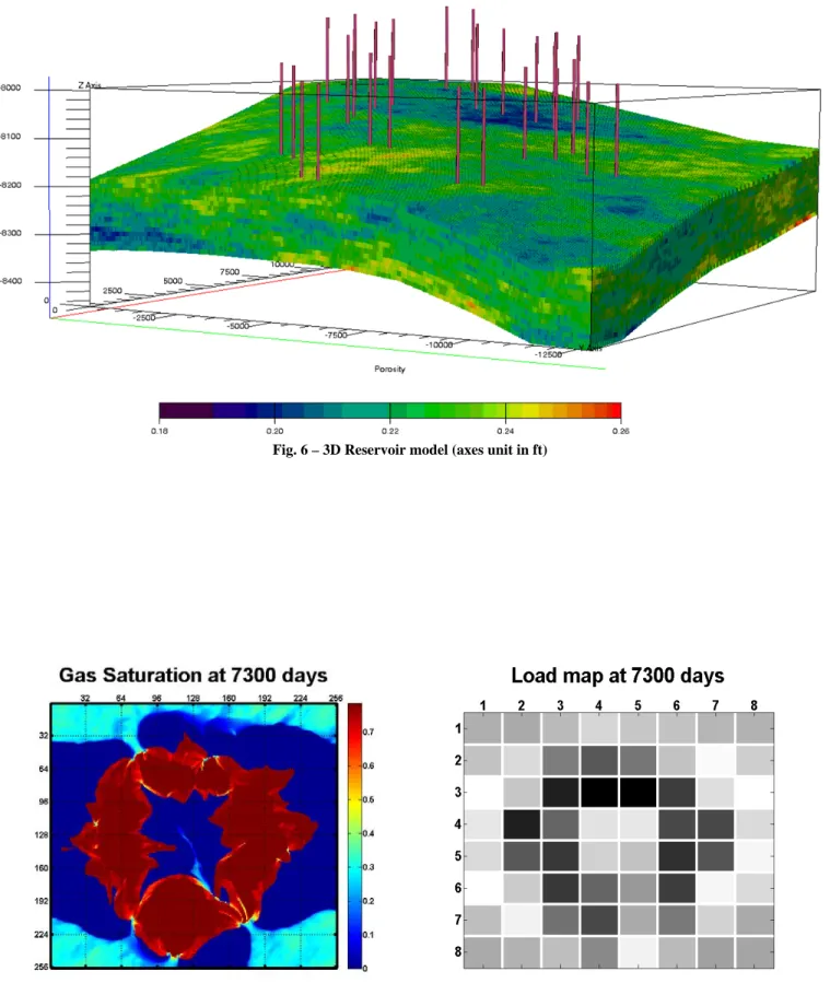
As depicted in Fig. 6, a 3D reservoir model using a corner point grid is used as the test case. It contains 15 vertical layers and each layer has 256ൈ256 grid blocks. Thus, it has totally 983,040 grid blocks. This reservoir has about areal dimension of about 3760 acres and 150 ft thickness. 14 gas injectors and 14 producers are perforated throughout all of the layers. Porosity is generated by sequential Gaussian simulation and permeability is obtained by correlation. This reservoir model contains 12 hydrocarbon components besides water. The properties of these components are provided in Table 6. In Table 6, MW, TC, PC, W, ZC, VPARM are molecular weight, critical temperature, critical pressure, Pitzer accentric factor, critical Z-factor, and volumetric shift parameter, respectively. A 20-year production/injection period is simulated for this model.
Table- 6 Properties of Components
Component MW TC (Rankine) PC (psi) W ZC VPARM
CO2 44.010 547.650 1071.30 0.2250 0.2750 0.02700 C1 16.040 343.040 667.800 0.0130 0.2900 -0.11800 C2 30.070 549.760 707.800 0.0986 0.2850 -0.10700 C3 44.100 665.680 616.300 0.1524 0.2770 -0.08477 C4 58.120 765.320 550.700 0.2010 0.2740 -0.06858 C5 72.150 845.370 488.600 0.2539 0.2690 -0.04103 C6+ 94.200 975.920 458.680 0.2695 0.2663 -0.00076 C8+ 116.00 1087.87 408.080 0.3328 0.2589 0.05973 C11+ 169.50 1223.01 305.180 0.4856 0.2546 0.08719 C15+ 232.60 1353.35 248.530 0.6436 0.2691 0.09684 C20+ 328.00 1458.35 227.270 0.7926 0.3165 -0.06104 C30+ 628.00 1670.24 168.570 1.0536 0.3676 -0.13829
The IMPES formulation is applied in this case. The key parameters used to control the equation of state convergence are residual norm of flash calculations, maximum residual of constant K-flash, and change in K-values for stability calculations, which are set to be 1.0e-6, 1.0e-6, and 1.0e-8, respectively. The jacobian is set to be recalculated only at selected grid blocks and K-value is set such that starting values cannot be borrowed from neighbor grid blocks. The timing summary for this reservoir model in sequential execution is listed in Table 7. We can see that, for this case, the equation of state calculations consume almost 80% of the total computational time. It is this part of computation that we parallelize in this study.
Table – 7 Percent of time spent in each portion of sequential execution of the test case Portion of simulator Percent of time spent
Linear Solver 14%
Equation of State 79% Coefficient Setup 6%
Others 1% 2. Performance of MPI
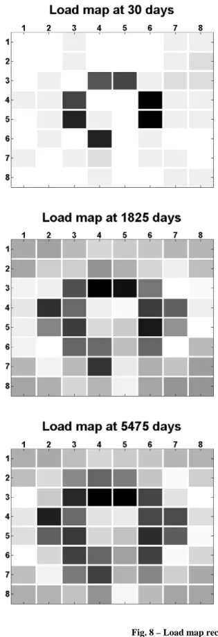
As has been discussed in previous sections, MPI implementation of a parallel equation of state is very likely to suffer dynamic load imbalance issues. Subdomains with phase changes or at critical conditions will dominate the execution time. To test the performance of an ordinary MPI implement with static decomposition, we run the case reservoir model using 64 physical processors. The model is divided into 64 subdomains using 2D domain decomposition, i.e. 8×8 decomposition. Depicted in the left picture of Fig. 7 is the gas saturation distribution of the top layer at 7300 days. The small squares that are separated by dash lines correspond to the decomposed subdomains. The saturation map is believed to be a strong indicator for processor load in the equation of state calculations. Shown in the right picture of Fig. 7 is the gray-scale-coded load map at 7300 days for the 8×8 set of physical processors. The darker the color is the higher the load is for a particular processor.
Indeed, there is a clear correlation between the saturation map and load map.
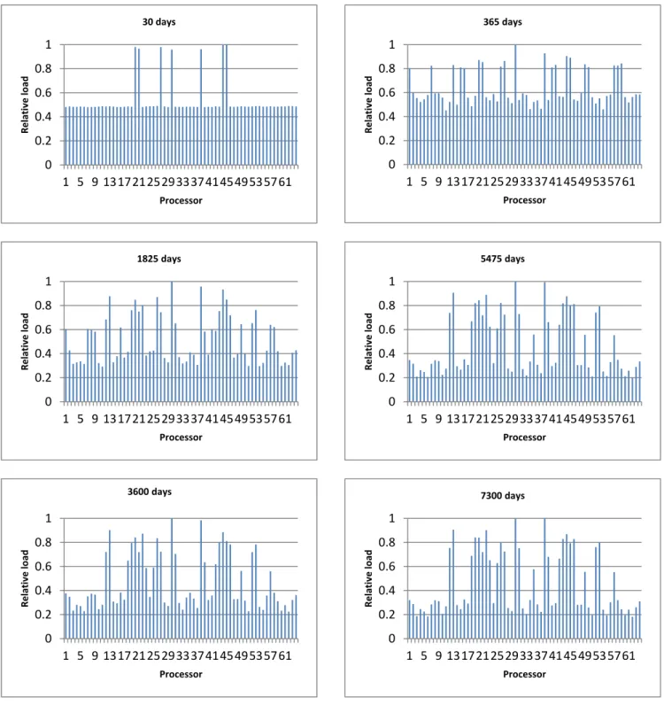
In addition, the load distribution of physical processors does not remain unchanged as simulation running. We explicitly show the load map at 30, 365, 1825, 3650, 5475 and 7300 days in Fig. 8. To better quantitatively understand the load imbalance, we also provide the column plots at these time snapshots in Fig. 9. Note that, the loads are normalized to the highest processor at each snapshot. Initially, at 30 days, the dark processors correspond to the subdomains that contain wells. Other processors are roughly equally loaded. This is easy to be understood since at 30 days most of the states changes happen near the wells. The load maps become complex at later time snapshots. Although the load maps do seem to be similar at 1825, 3650, 5475 and 7300 days, the imbalances and high-to-low load ratios are different. The imbalance is quantified by how much the load in most loaded processor is above the average load. The imbalances and high-to-low load ratios at these snapshots are listed in Table 8. It is should be noted that, since a star topology is applied such that the master processor scatters data to and gathers results from all of the slave processors, the master processor will have significantly more message send-receives. For this reason, the load results are chosen to only reflect the actual equation of state computations. It can be seen from Table 8 that imbalance and high-to-low load ratio tend to increase with time.
Table 8 – Imbalance and high-to-low load ratio at selected days Time (days) Imbalance High-to-low load ratio
30 46% 2.08 365 36% 2.21 1825 48% 3.42 3600 52% 4.45 5475 53% 4.98 7300 55% 5.60
3. Performance of Processor Virtualization
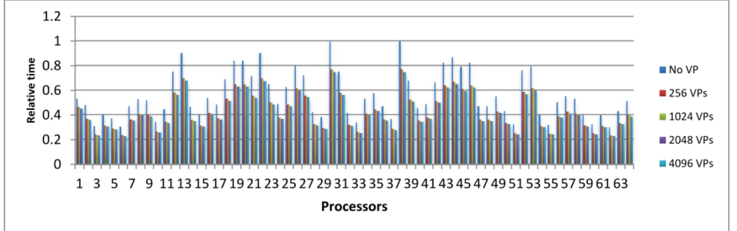
We first evaluate the effect of domain over-decomposition or processor virtualization on the case model. To perform this comparison we simply vary the number of VPs using a fixed number of physical processors, i.e. 64 processors in this case. It is expected that overhead due to handling extra user-level threads and communications will be brought in by increasing the processor virtualization ratio. However, there may still be benefits due to the implicit overlap of computation and communication and better cache utilization. For example, in this case model, when the master user-level thread blocks a receiving message, other VPs can still execute on the same physical processor; while in ordinary MPI execution, this physical processor will be held for receiving.
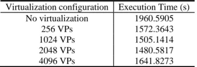
We compare the execution timings of equation of state of the case model at 7300 days with 64, 256, 1024, 2048, 4096 virtual processors, respectively. We consider the total elapsed time during equation of state, which incudes the data scattering, actual computation, and results gathering. These results are shown in Table 9. As it can been seen in Table 9, the execution time is reduced by 19.78% with 256 VPs, 23.23% with 1024 VPs, 24.48% with 2048 VPs, and 16.27% with 4096 VPs. It seems that there is an optimal number of VPs. The use of more VPs does not improve the performance further. To understand this behavior, we provide the column plot of the actual time of equation of state computation using different VPs in Fig. 10. As we can see from Fig. 10, the load imbalance pattern remains unchanged for different processor virtualization ratios. The reduction in computational time is believed to be the result of better cache utilization since the subdomain size becomes much smaller if high processor virtualization ratio is applied. The reduction of time in data scattering and gathering is the result of overlap of computation and communication when the master VP performs sending and receiving of messages. Thus, the observed effects of processor virtualization are the combination of results from better cache utilization and overlap of computation and communication. However, the performance improvement is limited by the server load imbalance in equation of state computations.
Table 9 Execution time of equation of state on 64 processors Virtualization configuration Execution Time (s)
No virtualization 1960.5905
256 VPs 1572.3643
1024 VPs 1505.1414
2048 VPs 1480.5817
4096 VPs 1641.8273
4. Performance of Dynamic Load Balancing
As revealed in last section, merely domain over-decomposition can only improve the performance to some extent (24.48% in this case). A dynamic load balance scheme must be applied for better performance enhancement. Fortunately, load balancing becomes much easier in the virtualized implementation of MPI, since the over-decomposed VPs are ready to be migrated to
mitigate load imbalance. Thanks to the particular feature of equation of state, there is only computation involved and no communication needed between VPs. As a result, a dynamic load balancer that only handles computation should be enough for this kind of application. For this reason, we choose GreedyLB and RefineLB to balance the load during parallel equation of state computation. Listed in Fig.11 are the timing results of each processor before and after implementation of the abovementioned load balancers. The reference timing without load balancer is shown in Fig. 11a. Clearly, only a few of processors dominate the execution time, while others are idle. The results of GreedyLB and RefineLB are provided in Fig. 11b and Fig. 11c, respectively. Apparently, the performances of GreedyLB and RefineLB are distinct. GreedyLB balances the load very well. Indeed, by design GreedyLB algorithm always grabs the heaviest unassigned VPs and assigns it to the currently least loaded physical processor until a balance is reached. In contrast, as shown in Fig. 11c, RefineLB only balances the load to some extent and the imbalance trend seems to be unchanged, since the RefineLB algorithm tries to minimize the number of VPs to be migrated. RefineLB is only useful when only a small number of VP migrations is enough to reach balance. Nevertheless, GreedyLB is an ܱሺ݈ܰ݃ܰሻ algorithm, which implies that it is more expensive than RefineLB. This is confirmed by measuring the overhead cost of the load balancing scheme and VP migrations. It can be seen from Table 10 that GreedyLB is about 10 times more expensive than RefineLB in this example case:
Table 10 Load balancing overhead Load balancer Overhead (s)
GreedyLB 40.85 RefineLB 4.21
However, these overheads become negligible when comparing with the total execution time. This is attributed to the smart runtime system and overlap of VP migrations and computations, which help to hide migration overhead. To finalize our experiments, we provide the speedup improvement after applying the new technique introduced in this paper. It can be seen from Table 11 that the speedup using 64 physical processors is improved from 29.27 to 62.38.
Table 11 Speedup improvements for 64 processors Configuration Speedup
MPI 29.27
2048 VPs 38.73
2048 VPs + GreedyLB 62.38
Conclusions and Outlooks
In this paper, it is shown that load imbalance is the key performance limiter for parallel compositional simulation when using the IMPES formuation for reservoir simulation. This kind of load imbalance is often dynamic and highly unpredictable. Thus, a dynamic load balancing scheme must be implemented to improve parallel performance. However, adaptation of dynamic load balancers to an established legacy reservoir simulator can be challenging and requires a substantial amount of development time. This paper provides a promising shortcut to mitigate load imbalance yet with high efficiency. Built upon Charm++ and AMPI, this approach over-decomposes the underlying reservoir model into small chunks. A bundle of these chunks is then mapped to each physical processor as virtual processes or user-level threads. Based on this unique idea, we develop a new parallel equation of state computation capability on a legacy commercial comprehensive reservoir simulator. It is shown that domain over-decomposition and GreedyLB load balancer in together help to improve the speedup from 29.27 to 62.38 on 64 physical processors. This is because, by design, domain over-decomposition not only brings overlapping between communication and computation and better cache utilization, but also provides a natural framework for dynamic load balancing.
It should be noted that it is due to the particular feature of equation of state computation that GreedyLB provides excellent performance. Generally, inter-subdomain data exchange is not needed in this application. Thus, a balancer without considering communication is enough. If the abovementioned approach is applied to general reservoir simulations, clearly, other balancers should be implemented to considering inter-subdomain communication. A full adaption to a comprehensive reservoir simulator should be straightforward if an MPI version is in hand. The key in a successful implementation is the correct treatment of global and static variables.
This technique is only adapted to the parallel equation of state in a reservoir simulator. The impact on the linear solver should also be investigated before full implementation. Based on limited experiments, it appears that domain over-decomposition can improve Jacobi, Gauss-Seidel and CG iterative solvers’ parallel performances by 10%-20%. However, further research needs to be performed for more complex parallel preconditioners and linear solvers.
Acknowledgements
The first author would like to thank Dr. Gengbin Zheng of National Center for Supercomputer Application at UIUC and Dr. Eduardo Rodrigues of Federal University of Rio Grande do Sul for valuable helping on Charm++ and AMPI.
References
Anguille, L., Killough, J.E., Li, T.M.C, Toepfer, J.L. 1995. Static and Dynamic Load-balancing Strategies for Parallel Reservoir. Paper SPE 29102 presented at the SPE Symposium on Reservoir Simulation, San Antonio, Texas, 12-15.
February. http://dx.doi.org/10.2118/29102-MS.
Appleyard, J.R., Appleyard, J.D., Wakefield, M.A., Desitter, A.L. 2011. Accelerating Reservoir Simulators Using GPU Technology. Paper SPE 141402 presented at the SPE Reservoir Simulation Symposium, The Woodlands, Texas, 21-23
February. http://dx.doi.org/10.2118/141402-MS.
Bayat, M., Killough, J. 2013. An Experimental Study of GPU Acceleration for Reservoir Simulation. Paper SPE 163628 presented at the SPE Reservoir Simulation Symposium, The Woodlands, Texas, 18-20 February.
Bohm, E., Bhatele, A., Kale, L.V., Tuckerman, M.E., Kumar, S., Gunnels, J.A., Martyna, G.J. 2008. Fine Grained Parallelization of the CaParrinello ab initio MD Method on Blue Gene/L. IBM journal of Research and Development: Applications of Massively Parallel Systems, 52(½): 159-174
Cao, H., Tchelepi, H.A., Wallis, J.R., Yardumian, H. 2005. Parallel Scalable Unstructured CPR-Type Linear Solver for Reservoir Simulation. Paper SPE 96809 presented at the SPE Annual Technical Conference and Exhibition, Dallas, Texas, 9-12 October. http://dx.doi.org/ 10.2118/96809-MS.
Dean, R.H. and Lo, L.L. 1988. Simulation of Naturally Fractured Reservoirs. SPE RE 3(2): 633-648. SPE-14110-PA. http://dx.doi.org/10.2118/14119-PA.
Foltinek, D., Eaton, D., Mahovsky, J., Moghaddam, P., McGarry, R. 2009. Industrial-scale Reverse Time Migration on GPU Hardware. SEG Annual Meeting, Extended Abstract, 2009-2789.
Huang, C., Zheng, G., Kumar, S., Kale, L.V. 2006. Performance evaluation of adaptive MPI. In Proceedings of ACM SIGPLAN Symposium on Principles and practice of Parallel Programming, 29-31 March. http://dx.doi.org/10.1145/1122971.1122976.
Huang, C., Lawlor, O., Kale, L.V. 2003. Adaptive MPI. In Proceedings of the 16th International Workshop on Languages and Compilers for Parallel Computing.
Fung, L.S.K., Dogru, Ali H. 2007. Parallel unstructured solver methods for complex giant reservoir simulation. Paper SPE 106237 presented at the SPE Reservoir Simulation Symposium, Houston, Texas, 26-28 February. http://dx.doi.org/10.2118/106237-MS.
Jetley, P., Gioachin, F., Mendes, C., Kale, L.V., Quinn, T.R. 2008. Massively Parallel Cosmological Simulations with ChaNGa. In Proceedings of IEEE International Parallel and Distributed Processing Symposium. 14-18 April. http://dx.doi.org/10.1109/IPDPS.2008.4536319.
Jiao, X., Zheng, G., Lawlor, G., Alexander, P., Campbell, M., Heath, M., Fiedler, R. 2005. An Integration Framework for Simulations of Solid Rocket Motors. In 41st AIAA/ASME/SAE/ASEE Joint Propulsion Conference, Tucson, Arizona, 10-13 July.
Kale, L.V., Bohm, E., Mendes, C.L., Wilmarth, T., Zheng, G. 2008. Programming Petascale Applications with Charm++ and AMPI. in Petascale Computing: Algorithms and Applications. Bader, D., Ed. Chapman & Hall/CRC Press, pp. 421-441. Karypis, G. and Kumar, V. 1999. A fast and high quality multilevel scheme for partitioning irregular graphs. SIAM Hournal
on Scientific Computing, 20(1): 359-392.
Killough, J.E., Wheeler, M.F. 1987. Parallel Iterative Equation Solvers: an Investigation of Domain Decomposition Algorithms for Reservoir Simulation. Paper SPE 16021 presented at the SPE Symposium on Reservoir Simulation, San Antonio, Texas,1-4 February. http://dx.doi.org/10.2118/16021-MS.
Klie, H., Sudan, H., Li, R., Saad, Y. 2011. Exploiting Capabilities of Manycore Platform in Reservoir Simulation. Paper SPE 141265 presented at the SPE Reservoir Simulation Symposium, The Woodlands, Texas, 21-23 February. http://dx.doi.org/10.2118/141265-MS.
Lui, H., Yu, S., Chen, Z., Hsieh, B., Shao, L. 2012. Parallel Preconditioners for Reservoir Simulation on GPU. Paper SPE 152811 presented at the SPE Latin America and Caribbean Petroleum Engineering Conference, Mexico City, Mexico, 16-18 April. http://dx.doi.org/10.2118/152811-MS.
Rodrigues, E.R., Navaux, P.O.A., Paneta, J., Fazenda, A., Mendes, C.L., Kale, L.V. 2010. A Comparative Analysis of Load Balancing Algorithms Applied to a Weather Forecast Model. In Proceeding SBAC-PAD ’10 Proceedings of the 2010 22nd International Symposium on Computer Architecture and High Performance Computing. Petrópolis, Rio de Janeiro, Brazil. 27-30 October. http://dx.doi.org/10.1109/SBAC-PAD.2010.18.
Rodrigues, E.R., Navaux, P.O.A., Panetta, J., Mendes, C.L. 2010. A New Technique for Data Privatization in User-level Threads and Its Use in Parallel Applications. In ACM 25th Symposium on Applied Computing (SAC), Sierre, Switzerland. 22-26 March. http://dx.doi.org/10.11451774088.1774540.
Rodrigues, E.R. 2012. Thread local storage enabled GFortran. Private Communication.
Sherman, A.H. 1992. A Hybrid Approach to Parallel Compositions Reservoir Simulation. Paper OTC 6829 presented at the Offshore Technology Conference, Houston, Texas, 4-7 May. http://dx.doi.org/10.4043/6829-MS.
Shuttleworth, R., Maliassov, S., Zhou, H. 2009. Partitioners for Parallelizing Reservoir Simulations. Paper SPE 119130 presented at the SPE Reservoir Simulation Symposium, The Woodlands, Texas, 2-4 February. http://dx.doi.org/10.2118/119130-MS.
Zhang, K., Wu, Y.S., Pruess, K., Elmroth, E. 2001. Parallel Computing Techniques for Large-scale Reservoir Simulation of Multi-component and Multiphase Fluid Flow. Paper SPE 66343 presented at the SPE Reservoir Simulation Symposium, Houston, Texas, 11-14 February. http://dx.doi.org/10.2118/66343-MS.
Zheng, G. 2005. Achieving High Performance on Extremely Large Parallel Machines: Performance Prediction and Load Balancing. Ph.D. Dissertation, University of Illinois at Urbana-Champaign, Illinois (Dec 2009).
Zheng, G., Lawlor, G.O.S., Kale, L.V. 2006. Multiple Flows of Control in Migratable Parallel Programs. In 2006 International Conference on Parallel Processing Workshops (ICPPW’06). Columbus, Ohio, 14-18 August. http://dx.doi.org/10.1109/ICPPW.2006.58.
Zheng, G., Negara, S., Mendes, C., Rodrigues, E., Kale, L. 2011. Automatic Handling of Global Variables for Multi-threaded MPI programs.In Proceeding ICPADS ’11 Proceedings of the 2011 IEEE 17th International Conference on Parallel and Distributed Systems. Tainan, Taiwan, 7-9 December. http://dx.doi.org/10.1109/ICPADS.2011.33.
Fig. 1 – Programmer view vs. real implementation of over-decomposed objects (adapted from Huang et al. (2006))
Fig. 2 – MPI “processes” are implemented as virtual processes (user-level threads) in AMPI (adapted from Huang et al. (2006))
Real Physical Processors MPI “processes” as virtual processes
Processor 0 Processor 1
Programmer View
Real Implementation
Fig. 3 – Domain over-decomposition. On the left, the domain is over-decomposed into smaller subdomains. The same grid fill pattern denotes the same physical processor
Fig. 4 – Migration of VP
Fig. 6 – 3D Reservoir model (axes unit in ft)
Fig. 9 – Column plots of load at various time snapshots 0 0.2 0.4 0.6 0.8 1 1 5 9 13172125293337414549535761 Relative load Processor 30 days 0 0.2 0.4 0.6 0.8 1 1 5 9 13172125293337414549535761 Relative load Processor 365 days 0 0.2 0.4 0.6 0.8 1 1 5 9 13172125293337414549535761 Relative load Processor 1825 days 0 0.2 0.4 0.6 0.8 1 1 5 9 13172125293337414549535761 Relative load Processor 3600 days 0 0.2 0.4 0.6 0.8 1 1 5 9 13172125293337414549535761 Relative load Processor 7300 days 0 0.2 0.4 0.6 0.8 1 1 5 9 13172125293337414549535761 Relative load Processor 5475 days
Fig. 10 – Column plots of load for different number of virtual processors
Fig. 11 – a: time column plot without load balancer; b: time column plot with RefineLB; c: time column plot with GreedyLB
0 0.2 0.4 0.6 0.8 1 1.2 1 3 5 7 9 11 13 15 17 19 21 23 25 27 29 31 33 35 37 39 41 43 45 47 49 51 53 55 57 59 61 63 Relative time Processors No VP 256 VPs 1024 VPs 2048 VPs 4096 VPs 0 500 1000 1500 2000 1 5 9 13 17 21 25 29 33 37 41 45 49 53 57 61 Time (s) Processors
a: Without Load Balancing
0 200 400 600 800 1000 1200 1400 1600 1 9 17 25 33 41 49 57 Time (s) Processors b: RefineLB 0 200 400 600 800 1000 1 5 9 13 17 21 25 29 33 37 41 45 49 53 57 61 Time (s) Processors c: GreedyLB