Model-based and Learned Semantic Object Labeling in 3D Point Cloud
Maps of Kitchen Environments
Radu Bogdan Rusu, Zoltan Csaba Marton, Nico Blodow, Andreas Holzbach, Michael Beetz
Intelligent Autonomous Systems, Technische Universit¨at M¨unchenBoltzmannstr. 3, Garching bei M¨unchen, 85748, Germany {rusu,marton,blodow,holzbach,beetz}@cs.tum.edu
Abstract— We report on our experiences regarding the acqui-sition of hybrid Semantic 3D Object Maps for indoor household environments, in particular kitchens, out of sensed 3D point cloud data. Our proposed approach includes a processing pipeline, including geometric mapping and learning, for pro-cessing large input datasets and for extracting relevant objects useful for a personal robotic assistant to perform complex manipulation tasks. The type of objects modeled are objects which perform utilitarian functions in the environment such as kitchen appliances, cupboards, tables, and drawers. The resulted model is accurate enough to use it in physics-based simulations, where doors of 3D containers can be opened based on their hinge position. The resulted map is represented as a hybrid concept and is comprised of both the hierarchically classified objects and triangular meshes used for collision avoidance in manipulation routines.
I. INTRODUCTION
Autonomous personal robots performing everyday manip-ulation tasks such as setting the table and cleaning up in human living environments must know the objects in their environments: the cupboards, tables, drawers, the fridge, the dishwasher, the oven, and so on.
The knowledge about these objects must include de-tailed information about the objects geometry, and structural knowledge as: a cupboard consists of a container box, a door with hinges and a handle. It even needs functional knowledge that enables the robot to infer from the position of a handle on a door the side to which the door opens.
Fig. 1. A snapshot of our kitchen lab: 16 registered scans shown in intensity (grayscale), comprising roughly 15 millions of points. The world coordinate
system depicted on the bottom left showsX with the red color,Y with
green, andZwith blue.
We propose to extend the robot’s mechanisms for the acquisition of environment models in order to acquire these kinds of information automatically. To this end, we investi-gate the following computational problem: given a 3D point cloud model of an environment as depicted in Figure 1, segment the point cloud into subsegments that correspond to relevant objects and label the segments with the respective category label (see Figure 2).
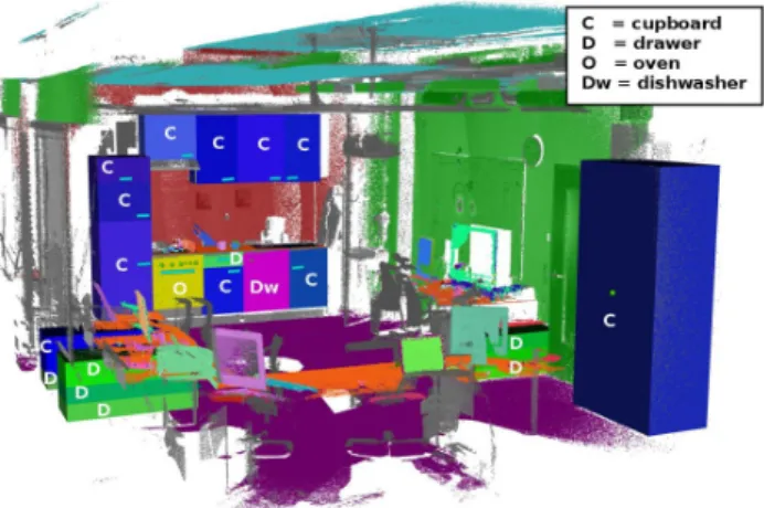
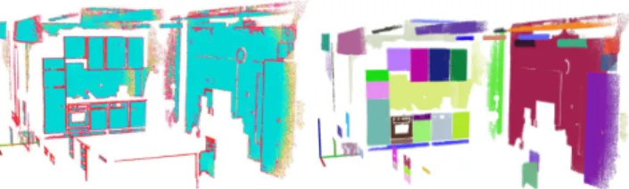
Fig. 2. Semantic 3D Object Map of an indoor kitchen environment.
The representative planar areas are shown in different colors (tables -orange, floor - dark purple, walls - green and red, ceiling - cyan), and 3D cuboid containers are marked with their appropriated labels (cupboard, drawer, oven, etc). The remaining unclassified points are shown in gray. (For interpretation of the references to color in this figure legend, the reader is referred to the web version of this article.)
The resultant labeled object model1 is meant to represent
the environment as best as possible given the geometry present in the input data, but its accuracy does not have to be absolute with respect to the true world model. Instead, the object model is considered as an intermediate representation that provides candidate objects which are to be validated through subsequent processing steps. These steps include vision based object recognition, active exploration like for example opening the drawers and doors that were suggested, and classifications based on the role that an object has in a certain activity (i.e. activity recognition). For this reason, the main objective of our mapping system is to compute the model as quickly as possible using solely the geometric in-formation contained in the point cloud, and have results that
approximate the true world model. However our experience as well as the illustration in Figure 2 suggests that most objects can be segmented and labeled correctly.
These concepts constitute incremental work from our previous work [1], and form the basis of our 3D mapping system. The key contributions of the research reported in this paper include the following ones: i) a multi-LoD (Level of Detail) planar decomposition mechanism that exploits the regularities typically found in human living environ-ments; ii) efficient model-fitting techniques for the recog-nition of fixtures (handles and knobs) on cupboards and kitchen appliances; and iii) a learning scheme based on a 2-levels geometric features extraction for object classes in the environment.
The remainder of this paper is organized as follows. The next section briefly describes related work, followed by the architecture of our mapping system in Section III. Section IV present the planar decomposition, region growing, and level-1 feature estimation, while in Section V we discuss the fixture segmentation for furniture candidates and the level-2 feature estimation. Section VI presents the machine learning model used to train the features, followed by a discussion of the system’s overall performance in Section VII. We conclude and give insight on our future work in Section VIII.
II. RELATEDWORK
The concept of autonomously creating maps with mobile robot platforms is not new, but so far it was mostly used for the purpose of 2D robot localization and navigation, with few exceptions in the area of cognitive mapping [2], [3], but also including [4]–[9]. A workaround is represented by maps built using multimodalities, such as [2], [10], [11], where 2D laser sensors are used to create a map used for navigation and additional semantics are acquired through the use of vision. For example in [10] places are semantically labelled into corridors, rooms and doorways. The advantages of these representations is straightforward: it keeps computational costs low enough and base their localization and pose estimation on the well known 2D SLAM (Simultaneous Localization and Mapping) problem, while the problem of place labeling is solved through the usage of feature descriptors and machine learning. However, by reducing the dimensionality of the mapping to 2D, most of the world geometry is lost. Also, the label categories need to be learned a priori through supervised learning and this makes it unclear whether these representations scale well. [8] classifies 3D sensed data from a laser sensor into walls, floor, ceiling, and doors, but their segmentation scheme relies on simple angular thresholds. In [9], the authors use a graph representation to detect chairs, but the relation descriptions are manually estimated, and thus it is unclear whether the proposed method scales. The work in [12] is closer to our approach as they use probabilistic graphical models such as Markov Random Fields to label planar patches in outdoor urban datasets. Their work is based on [13], [14], which define point-based 3D descriptors and classify them with respect to object classes such as: chairs, tables, screens, fans,
and trash cans [14], respectively: wires, poles, ground, and scatter [13].
Our mapping concept falls into the category of semanti-cally annotating 3D sensory data with class labels, obtained via supervised learning or learned by the robot through expe-rience, to improve the robot’s knowledge about its surround-ings and the area in which it can operate and manipulate. The resulting models do not only allow the robot to localize itself and navigate, but are also resources that provide semantic knowledge about the static objects in the environment, what they are, and how they can be operated. Thus, static objects in the environment such as cupboards, tables, drawers, and kitchen appliances are structurally modeled and labeled, and the object models have properties and states. For example, a cupboard has a front door, handles and hinges, is a storage place, and has the state of being either open or closed.
III. SYSTEMOVERVIEW
We approach the map learning problem by designing a 2-levels geometric feature set for a machine learning classifier, that is capable of generating labeled object hypotheses only using the geometric data contained in the point clouds while scanning the environment.
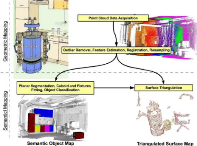
Figure 3 presents the overall architecture of our system. The integration of individual point cloud scans into the hybrid model follows the geometrical processing pipeline described in [1], [15], and includes: statistical gross outlier removal, feature estimation for each point in the dataset, a 2-step registration [16], and finally a local resampling of the overlapping areas between scans [1]. Their result is an improved point data model, with uniformly resampled 3D coordinates, and partially noiseless. This constitutes the input to the Semantic Mapping system. Since these general geometric mapping topics have already been covered in our previous work [1], [15], [16], they fall outside the scope of this paper.
Fig. 3. The architecture of our mapping system, and the 2 different types of maps produced. The input data is provided from the laser sensors installed on the robot’s arms via the Point Cloud Data Acquisition module, and is
processed through a Geometric Mapping pipeline resulting in aPCD world
model[1]. This model constitutes the input for the separate components of the Semantic Mapping module.
The term hybrid mapping refers to the combination of different data structures in the map, such as: points, triangle meshes, geometric shape coefficients, and 2D general poly-gons. Different tasks require different data structures from this map. For example, 3D collision detection usually re-quires either a triangle mesh representation or a voxelization of the underlying surface, while object classification might use the geometric shape coefficients. The hybrid Semantic Object Map in our implementation is comprised of 2 different types of maps:
• a Static Semantic Map comprised of the relevant parts of the environment including walls, floor, ceiling, and all the objects which have utilitarian functions in the en-vironment, such as fixed kitchen appliances, cupboards, tables, and shelves, which have a very low probability of having their position in the environment changed (see Figure 2);
• a Triangulated Surface Map, used for 3D path planning,
and collision avoidance for navigation and manipula-tion, using the techniques presented in [17].
The Semantic Mapping pipeline includes:
• a highly optimized major planar decomposition step, using multiple levels of detail (LOD) and localized sampling with octrees (see Section IV-A);
• a region growing step for splitting the planar compo-nents into separate regions (see Section IV-B);
• a model fitting step for fixture decomposition (see Section V-A);
• finally a 2-levels feature extraction and classification step (see Sections IV-C and V-B).
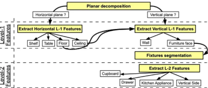
Figure 4 describes the 2-levels feature extraction and classification framework employed in our Semantic Mapping system. Instead of learning a single global model, we make use of proven geometrical techniques for splitting the data into clusters first, and compute separate features and a separate model for each of these clusters. The two defined level-1 clusters are composed of the horizontal planes, and the vertical planes respectively. By treating them separately, we simplify the features that need to be computed, remove false positives, and in general improve the classification results. Additionally, once we obtain a set of furniture faces labels from the classifier for vertical planes, we pro-ceed at extracting object fixtures (e.g. handles and knobs) and estimate a level-2 set of features which will help at separating furniture object types into drawers, cupboards, kitchen appliances, and vertical side faces respectively. A final advantage of this scheme is that we do not need to estimate all possible features for all planar candidates, but rather proceed at segmenting and computing features as needed, starting with simple ones (i.e. horizontal planes). Therefore, the overall system will benefit from a reduced computational complexity.
IV. PLANARDECOMPOSITION ANDLEVEL-1 FEATURE
ESTIMATION
The Semantic Object Map includes semantically annotated parts of the environment, which provide useful information
Planar decomposition Planar decomposition Fixtures segmentation Fixtures segmentation L e ve l-1 L ev el -1 F ea tu re s F e a tu re s
Extract Horizontal L-1 Features Extract Horizontal L-1 Features
Horizontal plane ? Horizontal plane ?
Extract Vertical L-1 Features Extract Vertical L-1 Features
Vertical plane ? Vertical plane ?
Shelf
Shelf TableTable FloorFloor CeilingCeiling WallWall Furniture faceFurniture face
L ev e l-2 L e ve l-2 F e a tu re s F e atu re
s Extract L-2 FeaturesExtract L-2 Features
Drawer Drawer Cupboard Cupboard
Kitchen Appliance
Kitchen Appliance Vertical SideVertical Side
Fig. 4. The 2-levels feature extraction and object classification framework
used in our mapping system.
for our mobile personal assistant robot in fulfilling its tasks. These parts are thought of as being unmovable or static, that is with a very low probability of having their position changed in the environment, though this is not a hard constraint for our system, in the sense that model updates are possible. To separate the objects functions, we devised three categories:
• structural components of the environment: walls, floor, ceiling;
• box-like containers which can contain other objects and have states such as open and closed: cupboards, drawers, and kitchen appliances;
• supporting planar areas: tables, tops of sideboards, shelves, counters, etc.
After the Geometric Mapping processing steps are applied on the raw scanned data, as shown in in Figure 3, the resultant point data model is transformed into the world coordinate frame, with theZ-axis pointing upwards. Figure 1 presents a 360◦ view, comprised of 16 registered scans of our kitchen lab. The world coordinate frame is presented on the left side of the figure, and depicts the general XY Z directions (X - red,Y - green, Z - blue).
A subsequent processing step is to segment the pointcloud into planar areas. Once all the major planar areas are found, and split into regions, we employ a 2-levels feature extraction and classification scheme (see Figure 4).
A. Planar Segmentation
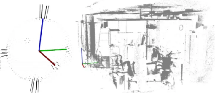
The assumption that our kitchen environment is mostly planar and can thus be decomposed into areas of interest using plane fitting techniques can be verified by looking at the Extended Gaussian Image (EGI) of the point cloud. As presented in the left part of Figure 5, most of the estimated point normals are found as being parallel with the principal XY Z directions, accounting for approximately 85% of the entire dataset. These exact numbers are not important as they will vary for other datasets, but in general they will prove the planarity tendency in indoor environments.
The planar model decomposition in the pointcloud data with near realtime performance, is achieved using a hier-archical multi-LoD (Level of Detail) scheme. Instead of using the entire data, we decompose the cloud using an octree scheme, and perform a RMSAC [18] (Randomized M-Estimator SAmple Consensus) based search for planar areas,
Fig. 5. Left: the Extended Gaussian Image (EGI) of the point cloud dataset. As seen, most of the estimated point normals are found around the principal
XY Z directions, accounting for approximately 85% of the entire dataset.
Right: the remaining points after major planar area segmentation in our kitchen dataset.
using the centroid of the leaves at the highest levels of detail in the tree (see Figure 6). To optimize the search even further, we make use of the estimated point normals while rejecting planar candidates.
Fig. 6. Two different levels of detail representing approximately 1% (level
8), respectively 0.2% (level 7) of the total number of points from the original dataset, created using an octree.
The multi-LoD scheme uses a localized sampling strategy. The first sample point p1 is chosen randomly from the complete point cloud. Then a octree levellis picked, which determinesC, the octree cell at levellthat containsp1. The
other two samples points p2,p3 are then drawn from this
cell. The probability of finding a planar modelMof size n can be expressed as follows:
Plocal(n) = n
N · P(p2,p3∈ M|p2,p3∈ C), (1) where the fraction denotes the probability for picking the first sample point fromM. The second term depends on the choice ofC, the properties of the point cloud and its octree. Assuming that there exists a cellCat some levell0such that
half of the points contained therein belong toM, the second term in Equation 1 can be rewritten as:
P(p2,p3∈ M|p2,p3∈ C) = |C|/2 2 |C| 2 ≈ 1 2 2 . (2)
since the probability of selecting the correct levell0 is d1,
whereddenotes the cell of the octree, equation 1 transforms into:
Plocal(n) = n
4N d (3)
If we were sampling all three points uniformly from the point cloud, the corresponding probability could be estimated as follows: (Nn)3, so the described sampling strategy im-proves that probability by a factor of 41d(Nn)2.
Once a plane model is computed at a certain level of detail, we refine its equation by including points from a higher octree level, and refit the model. Once all the levels have been exhausted we refine the resultant equation by including the original points in the scan. This scheme has the advantage that it constraints the rough planar equation from the beginning and computes an initial solution very early, while keeping the overall computational costs low.
Since the world coordinate frame is defined with the Z axis pointing upwards, in general we are always interested in dividing the planar models into two categories:
• horizontal planes, i.e. those whose normal is parallel with theZ axis;
• verticalplanes, i.e. those whose normal is perpendicular to theZ axis.
The first category will include structural components of the environment such as the floor and the ceiling, as well as planar areas which can support movable objects, such as tables, shelves, or counters (see Figure 7 left). The second category will devise the walls of the room, and all the faces of the furniture and kitchen appliances in the room (see Figure 7 right).
Fig. 7. Left: all horizontal planes found in the scene; right: all vertical
planes found in the scene.
B. Region Growing
After all the planar areas have been found, our pipeline proceeds at breaking the resultant regions into smaller parts using a region growing method. The algorithm is based on two factors, namely: i) the Euclidean distance between neighboring points, and ii) the changes in estimated surface curvature between neighboring points. The second factor is enforced by the use of boundary points, which will be considered as having an infinite curvature, and thus act as stoppers for the region growing algorithm.
To do this, first the boundary points of each region are computed as explained in [1]. The left part of Figure 8 presents the resultant boundary points for the vertical planar areas presented in the right part of Figure 7. Then, a random non-boundary point p is chosen and added to a list of seed points, and a search for its k closest 3D neighbors is performed. Each neighboring pointpkis individually verified whether it could belong to the same region as the seed point and whether it should be considered as a seed point itself at a future iteration of the algorithm. A region is said to be completewhen the list of seed points for the current region is empty and thus all point checks have been exhausted.
In contrast to our previous implementation in [1], the new region growing algorithm expands the regions until boundary
Fig. 8. Left: vertical planar areas shown with their estimated boundary points (marked with red); right: the resultant filtered regions after segmen-tation. (For interpretation of the references to color in this figure legend, the reader is referred to the web version of this article.)
points are hit instead of looking at the estimated surface curvature at each point. This has the advantage that we do not need any additional computations or curvature thresholds. A second optimization uses an octree decomposition to speed up the region growing, that is, if no boundary points are found within an octree leaf, all points are automatically added to the current region. A final filtering step is applied to remove bad regions, such as the ones where the number of boundary points is larger than the number of points inside the region. The segmentation results are shown in the right part of Figure 8.
C. Extracting Level-1 features
As presented in Figure 4, our mapping scheme implements two sets of geometric features at level-1, one for horizontal planes and one for vertical planes. Their description is given in Tables I and II. Throughout their definitions we use the notations|p−q| and|p−q|z, which denote the Euclidean distance between the pointspandqoverXY Z, respectively the length of the segment formed betweenp andq over Z. The first set of features will be computed for horizontal planes. Once a model that can separate horizontal planes into the object classes mentioned in Figure 4 is learned, the resultant ceiling and floor object models will be used to generate the level-1 features for vertical planes.
TABLE I
LEVEL-1FEATURES FOR HORIZONTAL PLANES.
Feature Notation Description
Height Hh the height of the planar model onZwith respect
to the world coordinate frame
Length Lh the length along the first principal component
Width Wh the length along the second principal component
The vertical planar classification separates walls from furniture candidates. Since we already know the planar equations of the ceiling and the floor from the horizontal planar classification, we use these to determine the height of the vertical region with respect to them. The goal is to differentiate between walls and other types of vertical planes which will be considered unanimously as possible furniture candidates. Therefore, the vertical regions which contain points close to the ceiling might be classified as walls. In our case, it is not extremely important if these are actual walls or not – what matters is that those regions are high enough that they are unreachable by the robot anyway. Notice that the regions do not have to be continuous, as
all the points which have the same plane equation will be marked as walls.
TABLE II
LEVEL-1FEATURES FOR VERTICAL PLANES.
Feature Notation Description
Height Hv the actual length along theZaxis (i.e.
|Mz−mz|whereMz andmz are
the points with the maximum
respec-tively minimumZvalues)
Floor distance Dfv the distance to the floor model (i.e.
|mz −pf|z where mz is the point
with the minimumZvalue, andpf is
a point on the floor)
Ceiling distance Dc
v the distance to the ceiling model (i.e.
|mz−pc|zwheremzis the point with
the maximumZvalue, andpcis a point
on the ceiling)
Width Wv the length along the biggest principal
component, excludingZ
Since the feature spaces are relatively simple, the choice of using the right machine learning classifier is greatly simplified. In our implementation, we decided to use a probabilistic undirected graphical method for training the models, namely Conditional Random Fields (see Section VI).
V. FIXTURESEGMENTATION ANDLEVEL-2 FEATURE
ESTIMATION
The classifiers constructed using the level-1 features pre-sented in the previous section separate the planar regions into object classes such as tables and shelves (on horizontal) or walls and furniture faces (on vertical).
Following the architectural framework depicted in Fig-ure 4, our mapping pipeline employs a segmentation of fixtures (e.g. handles and knobs) on vertical planar regions classified as possible furniture faces.
A. Fixture Segmentation
For each of the classified furniture faces candidates, we perform a search for points lying in their vicinity, which could contain fixtures such as handles and knobs. The algorithm for extracting fixtures consists in the following steps:
• compute the boundary points of each furniture face candidate;
• obtain the 2 directions perpendicular to the normal of the planar area, and find the best (i.e. highest numbers of inliers) 4 oriented lines, 2 in one direction and 2 in the other direction using RMSAC;
• get the 4 points which form the 3D rectangle approxi-mating the planar region;
• get all points which are lying on this rectangle but are not inliers of the planar face and compute their boundary points;
• finally, fit 3D lines and 3D circles to these boundary
points using RMSAC, score the candidates, and select the ones which minimize the Euclidean distance error metric. To refine the final shape parameters, we apply a non-linear optimization using Levenberg-Marquardt.
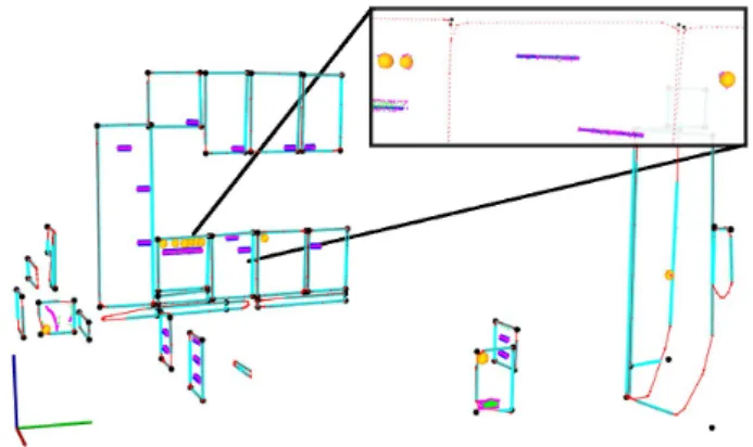
Figure 9 presents the segmentation and classification of all handles and knobs found on candidate furniture faces in the kitchen dataset presented in Figure 1.
Fig. 9. Segmentation and classification of fixtures (handles and knobs) on
furniture faces (see Figure 12). Handles are drawn with blue lines over their inlier points (in magenta), knobs with orange circles, and each planar area is bounded by 4 corners (in black) and 4 perpendicular lines (in cyan). The red dotted-lines represent the convex boundaries of each point region. (For interpretation of the references to color in this figure legend, the reader is referred to the web version of this article.)
B. Extracting Level-2 features
To differentiate between various possible furniture types, our mapping scheme implements a secondary type of features which are to be computed only for the vertical planar regions classified as furniture candidates. This set of features (see Table III) take into considerations constraints such as the number of handles and knobs present as lying on the planar region, as well as the distance between the center of the fixture and the center of the region.
TABLE III
LEVEL-2FEATURES FOR FURNITURE CANDIDATES.
Feature Notation Description
Height Hf the height of the furniture candidate
Width Wf the width of the furniture candidate
Nr. handles Nh the number of handles present on the
fur-niture candidate
Nr. knobs Nk the number of knobs present on the
furni-ture candidate
Min distance Dm the minimum distance between the center
of the planar face and the closest fixture (handle or knob)
Following the classification results for object types which employ fixtures towards one of the edges of the planar face supporting them (e.g. cupboards), our system will estimate the door opening hinge as being on the opposite edge.
VI. LEARNINGOBJECTCLASSES
We use Conditional Random Fields for the classification of our models. CRFs have mostly been used for segmenting and labeling sequence data [19] but have lately shown excellent results in other research areas as well. A Conditional Random Field is an undirected graphical model with vertices and edges. In contrast to generative graphical models, like Naive Bayes or Hidden Markov Models, a Conditional Random Field is a so called discriminative graphical model which
doesn’t represent a joint probability distribution p(x, y). Instead it uses a conditional probability distributionp(y|x)to provide a method to reason about the observationsxand the classification labely. The performance outcome of generative models often suffer from potentially erroneous independence assumptions made during modeling the observations x in connection to the labelsy. By using a discriminative graph-ical model like Conditional Random Fields, there is no need in modeling the features of y at all, which results in a superior classification speed and performance compared to generative models.
Applying the product rule and the sum rule on the condi-tional probabilityp(y|x), we get:
p(y|x) = p(y, x) p(x) = p(y, x) P y0p(y0, x) = Q c∈Cψc(xc, yc) P y0 Q c∈Cψc(xc, y0c) (4) where the factorsψcare the potential functions of the random variablesvC within a cliquec∈C.
Finally we can derive a general model formulation for Conditional Random Fields [20]:
p(y|x) = 1 Z(x) Y c∈C ψc(xc, yc), Z(x) = X y0 Y c∈C ψc(xc, y0) (5) By defining the factorsψ(y) =p(y)andψ(x, y) =p(x|y) we can derive an undirected graph with state and transition probabilities. The potential functions ψc can be split into edge potentialsψij and node potentials ψi as follows:
p(y|x) = 1 Z(x) Y (i,j)∈C ψij(yi, yj, xi, xj) N Y i=1 ψi(yi, xi) (6)
where the node potentials are ψi(yi, xi) = exp X L (λLixi)yLi ! (7) and the edge potentials are
ψij(yi, yj, xi, xj) = exp X L (λijxixj)yiLy L j ! (8) where λi represents the node weights and λij the edge weights. Learning in a Conditional Random Field is per-formed by estimating these weightsλi ={λ1i, . . . , λ
L i}and
λij={λ1ij, . . . , λ
L
ij}. Conditional Random Fields are trained using supervised learning, that means during the learning step the data input and output is known and used to maximize the log-likelihood ofP(y|x)[21]. y1 Hh Lh Wh Features Classification output y2 Hv Dvc W v Dvf H f Wf Nh Nk Dm y3
Fig. 10. From left to right: CRF for model 1 (Horizontal L-1 Features), 2
Figure 10 shows the Conditional Random Fields for our three different models. Each of the models’ features is used as an input variable. The variable nodes are named after the corresponding notations in Tables I, II, and III.
VII. DISCUSSIONS ANDEXPERIMENTALRESULTS
An important factor in the classification accuracy of the CRF model, is the amount and type of training data used for learning. Due to physical constraints in moving our mobile robot to a different kitchen environment, or changing the kitchen furniture to obtain multiple datasets, the amount of training data available was small. To circumvent this prob-lem, we proceeded as follows: we created realistic kitchen models in our Gazebo 2 3D simulator, and used virtual scanning techniques, followed by synthetic data noisifica-tion to acquire addinoisifica-tional point clouds representing kitchen environments (see Figure 11). After acquiring a few of these datasets, we processed them through our pipeline and extracted the 2-levels features for training the CRF model. Table V presents a few examples of virtually scanned kitchen environments (left) and their respective fixture on furniture candidate faces segmentation (right).
Fig. 11. An illustration of the simulated 3D environments and the process
of acquiring training datasets, using the Gazebo 3D simulator.
The classification results of the trained CRF model for the kitchen dataset presented in Figure 1 are shown in Table IV. The table shows the recall, precision and F1-measure values of all labels and the macro-averaged statistic of each model. The item accuracy is based on the overall correct classified items against the wrong classified items in the test data set.
TABLE IV
PERFORMANCE OF THECRF MODELS
Horizontal planes Vertical planes Furniture candidates
Label Prec. Rec. F1 Prec. Rec. F1 Prec. Rec. F1
1 1.00 0.50 0.67 1.00 0.91 0.95 0.94 1.00 0.97 2 1.00 1.00 1.00 0.97 1.00 0.98 0.97 0.89 0.93 3 0.96 1.00 0.98 0.50 0.75 0.60 Macro accuracy 0.99 0.83 0.88 0.99 0.95 0.97 0.80 0.88 0.83 Item accuracy 0.97 0.98 0.91
The labels for the models given in the above table represent (in order): floor, tables, and ceiling (horizontal planes); walls, and furniture candidates (vertical planes); respectively cupboards, drawers, and kitchen appliances (fur-niture candidates). As it can be seen, the lowest accuracy
2Gazebo is a 3D simulator - http://playerstage.sourceforge.net
of the classification results is represented by the kitchen appliances. The variety in the models we trained our model with is simply too large, and our proposed level-2 features cannot capture the modeling process correctly. We plan to investigate this further by redesigning our features as well as using more training datasets.
Figure 12 presents the classification of vertical planar areas into walls (left) and furniture candidates (right) using the aforementioned CRF model.
Fig. 12. Vertical planar regions classified as: walls (left); furniture
candidates (right); for the dataset presented in Figure 1.
After classification, the resulted objects are incorporated into the map and using a XML-based representation, we can import them back in the Gazebo simulator, where it is possible to perform a validation of the estimated door hinges and object classes. Figure 13 presents the automatic environment reconstruction of the real world dataset.
Fig. 13. Left: automatic environment reconstruction of the real world
dataset from Figure 2 in the Gazebo 3D simulator; right: the estimation and evaluation of door hinges from geometry data.
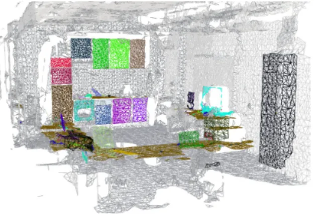
To support mobile manipulation and 3D collision avoid-ance, our mapping pipeline creates a second type of map comprised of triangular meshes: the Triangulated Surface Map. By using the acquired object classes, the surface recon-struction methods can be applied in parallel on each object separately, leading to the creation of a decoupled triangle map. The straightforward advantages of such a representation (see Figure 14 for an example) are that: a) changes in the world can be now be modelled separately on a subset of objects without loading or working with the rest; and b) it supports environment dynamics natively, as picking up an object from a table simply means moving the triangular mesh representing the object from the table into space, without the need to recreate it.
VIII. CONCLUSIONS ANDFUTUREWORK
We have presented a comprehensive system for the ac-quisition of hybrid Semantic 3D Object Maps for kitchen environments. Our hybrid mapping system includes 2 com-ponents, namely: i) a Semantic 3D Object Map which contains those parts of the environment with fixed positions
Fig. 14. Surface reconstruction example with mesh decoupling for all furniture candidates and objects supported by planar areas.
TABLE V
VIRTUALLY SCANNED TRAINING DATASETS.
Virtually scanned environment Segmentation and model fitting
and utilitarian functions (walls, floor, kitchen appliances, cupboards, tables, etc); and ii) a Triangulated Surface Map updated continuously. The Semantic Object Map is built by classifying a set of planar regions with estimated 3D geometrical features, and serves as a semantic resource for an assistant mobile personal robot, while the Triangulated Sur-face Map supports 3D collision detection and path planning routines for a safe navigation and manipulation.
As pure geometrical reasoning has certain limits, we plan to switch to a multimodality sensing approach, in which fast stereo cameras are combined with accurate laser mea-surements, and texture and color based reasoning will help disambiguate situations which geometry alone cannot solve. Acknowledgements: This work is supported by the CoTeSys (Cognition for Technical Systems) cluster of ex-cellence.
REFERENCES
[1] R. B. Rusu, Z. C. Marton, N. Blodow, M. Dolha, and M. Beetz, “Towards 3D Point Cloud Based Object Maps for Household
Envi-ronments,”Robotics and Autonomous Systems Journal (Special Issue
on Semantic Knowledge), 2008.
[2] S. Vasudevan, S. G¨achter, V. Nguyen, and R. Siegwart, “Cognitive
maps for mobile robots-an object based approach,” Robotics and
Autonomous Systems, vol. 55, no. 5, pp. 359–371, 2007.
[3] J. Modayil and B. Kuipers, “Bootstrap learning for object discovery,” in IEEE/RSJ International Conference on Intelligent Robots and Systems (IROS-04), 2004, pp. 742–747.
[4] Y. Liu, R. Emery, D. Chakrabarti, W. Burgard, and S. Thrun, “Using EM to Learn 3D Models of Indoor Environments with Mobile Robots,”
inICML, 2001, pp. 329–336.
[5] P. Biber, H. Andreasson, T. Duckett, and A. Schilling, “3D Modeling of Indoor Environments by a Mobile Robot with a Laser Scanner and
Panoramic Camera,” inIEEE/RSJ Int. Conf. on Intel. Rob. Sys., 2004.
[6] J. Weingarten, G. Gruener, and R. Siegwart, “A Fast and Robust 3D Feature Extraction Algorithm for Structured Environment
Reconstruc-tion,” inInt. Conf. on Advanced Robotics, 2003.
[7] R. Triebel, ´Oscar Mart´ınez Mozos, and W. Burgard, “Relational
Learning in Mobile Robotics: An Application to Semantic Labeling
of Objects in 2D and 3D Environment Maps,” inAnnual Conference
of the German Classification Society on Data Analysis, Machine Learning, and Applications (GfKl), Freiburg, Germany, 2007. [8] A. Nuechter and J. Hertzberg, “Towards Semantic Maps for Mobile
Robots,”Journal of Robotics and Autonomous Systems (JRAS), Special
Issue on Semantic Knowledge in Robotics, pp. 915 – 926, 2008. [9] M. Wuenstel and R. Moratz, “Automatic Object Recognition within
an Office Environment,” inCRV ’04: Proceedings of the 1st Canadian
Conference on Computer and Robot Vision, 2004, pp. 104–109. [10] O. M. Mozos, R. Triebel, P. Jensfelt, A. Rottmann, and W. Burgard,
“Supervised Semantic Labeling of Places using Information Extracted
from Laser and Vision Sensor Data,” Robotics and Autonomous
Systems Journal, vol. 55, no. 5, pp. 391–402, May 2007.
[11] L. Iocchi and S. Pellegrini, “Building 3D maps with semantic elements
integrating 2D laser, stereo vision and INS on a mobile robot,” in2nd
ISPRS International Workshop 3D-ARCH, 2007.
[12] I. Posner, M. Cummins, and P. Newman, “Fast Probabilistic Labeling
of City Maps,” in Proceedings of Robotics: Science and Systems,
Zurich, June 2008.
[13] D. Anguelov, B. Taskar, V. Chatalbashev, D. Koller, D. Gupta, G. Heitz, and A. Ng, “Discriminative learning of Markov random
fields for segmentation of 3d scan data,” inIn Proc. of the Conf. on
Computer Vision and Pattern Recognition (CVPR), 2005, pp. 169–176. [14] R. Triebel, R. Schmidt, O. M. Mozos, , and W. Burgard, “Instace-based AMN classification for improved object recognition in 2d and 3d laser
range data,” inProceedings of the International Joint Conference on
Artificial Intelligence (IJCAI), (Hyderabad, India), 2007.
[15] R. B. Rusu, Z. C. Marton, N. Blodow, M. E. Dolha, and M. Beetz,
“Functional Object Mapping of Kitchen Environments,” in
Proceed-ings of the 21st IEEE/RSJ International Conference on Intelligent Robots and Systems (IROS), Nice, France, September 22-26, 2008. [16] R. B. Rusu, N. Blodow, and M. Beetz, “Fast Point Feature Histograms
(FPFH) for 3D Registration,” inProceedings of the IEEE International
Conference on Robotics and Automation (ICRA), Kobe, Japan, May 12-17, 2009.
[17] Z. C. Marton, R. B. Rusu, and M. Beetz, “On Fast Surface
Recon-struction Methods for Large and Noisy Point Clouds,” inProceedings
of the International Conference on Robotics and Automation (ICRA), Kobe, Japan, May 12-17, 2009.
[18] P. Torr and A. Zisserman, “MLESAC: A new robust estimator with
application to estimating image geometry,” Computer Vision and
Image Understanding, vol. 78, pp. 138–156, 2000.
[19] J. Lafferty, A. Mccallum, and F. Pereira, “Conditional random fields: Probabilistic models for segmenting and labeling sequence data,” in Proc. 18th International Conf. on Machine Learning. Morgan Kaufmann, San Francisco, CA, 2001, pp. 282–289.
[20] R. Klinger and K. Tomanek, “Classical probabilistic models and con-ditional random fields,” Technische Universit¨at Dortmund, Dortmund,” Electronic Publication, 2007.
[21] E. H. Lim and D. Suter, “Conditional Random Field for 3D Point
Clouds with Adaptive Data Reduction,”Cyberworlds, International