Santhanam & Hartono/Lini<ing iT Capability to Firm Performance
RESEARCH NOTE
ISSUES IN LINKING INFORMATION TECHNOLOGY
CAPABILITY TO FIRM PERFORMANCE^
By: Radiiika Santhanam
DSiS Area, School of iVIanagement Gatton School of Business and
Economics University of Kentucky Lexington, Kentucky 40506-0034 U.S.A. [email protected] Edward Hartono
DSIS Area, School of Management Gatton School of Business and
Economics University of Kentucky Lexington, Kentucky 40506-0034 U.S.A. [email protected]
Abstract
The resource-based view has been proposed to investigate the impact of information technology (IT) investments on firm performance. Re-searchers have shown that a firm's ability to effectively leverage its IT investments by devei-oping a strong IT capability can result in improved
V.Sambamurthy was the accepting senior editor for this paper.
firm performance. We test the robustness of this approach and examine severai related issues. Our results indicate that firms with superior IT capability indeed exhibit superior current and sus-tained firm performance when compared to aver-age industry performance, even after adjusting for effects of prior firm performance. However, the differences in the results from various analyses suggest that the impact of "haio effects" and prior financial performance of firms must be taken into consideration in future tests of IT capability. Further, it is criticai to develop theoretically derived multidimensional measures of IT capabi-lity in order to continue to apply theRBV approach to assess the impact of IT investments on firm performance.
Keywords: Resource-based view, IT capability, firm pertormance
ISRL Categories: A i d 04, AF01.02, EI0102
Introduction
Corporations allocate resources to acquire IT-related products because it is assumed that these investments provide economic returns to a firm. Research studies to prove this premise have, however, generated mixed results, creating a
productivity paradox (Brynjolfsson and Hitt 1998;
Lucas 1999). This prompted an editorial comment in MIS Quarterly:
Santhanam & Hartono/Linking IT Capability to Firm Performance
It is the obligation of every IS profes-sional to understand the issues that surround the paradox...and each of us must then be prepared and willing to participate knowledgeably in the debate. (Ives1994, pp. 21-24)
To address this productivity paradox, a theory-based framework commonly referred to as the resource-based view (RBV) has been adopted. Based on this, Bharadwaj (2000) proposed that if firms can combine IT related resources to create a unique IT capability, it can result in superior firm performance. She demonstrated that the average performance of firms identified as possessing superior IT capability was significantly superior to the average performance of a matched set of firms.
A true test of a theory's usefulness depends on proper replications, extensions, and generaliza-tions (Rosenthal 1991; Tsang and Kwan 1999). Such replications play a central role in the construction of IS knowledge (Berthon et al. 2002) and can help build a much needed cumulative tradition in IS (Benbasat and Zmud 1999; Sambamurthy 2001). Because the RBV is in-creasingly being used to address a critical IS research issue, namely the productivity paradox, further investigation of this framework is neces-sary. Hence, the objective of this study is to test the robustness of the concept of IT capability and its relationship to firm performance, and to identify critical issues in the application of RBV to examine the productivity paradox.
Research Framework
Empirical evidence to unambiguously support the view that investments in IT-related resources enhance firm performance has been elusive (for a review, see Chan 2000). The inconsistencies observed among various studies have been attributed to variation in methods and measures used in the analyses (Hitt and Brynjolfsson 1996). Because the assessment ofthe economic impact of IT is of critical importance to IS researchers.
more research using unifying theory-based frame-works is necessary (Chan 2000; Ives 1994). Barney (1991) proposed that firms could obtain competitive advantages on the basis of corporate resources that are firm specific, valuable, rare, imperfectly imitable, and not strategically substitu-table by other resources. This is often referred to as the resource-based view (RBV) of a firm. Grant (1991) and Makadok (1991) emphasize that while resources by themselves can serve as the basic units of analyses, firms create competitive advantage by assembling these resources to create organizational capabilities. Makadok states that these firm-specific capabilities, embedded in organizational processes, provide economic returns because the firm is more effective than its rivals in deploying resources. IS researchers have adopted this capability notion of resources by arguing that competitors may easily duplicate investments in IT resources by purchasing the same hardware and software, and hence resources perse do not provide sustained compe-titive advantages. Rather, it is the manner in which firms leverage their IT investments to create unique capabilities that impact a firm's overall effectiveness (Clemons and Row 1991; Mata et al. 1995). Using this RBV framework, firms can devise strategies to create and sustain advan-tages from investments in IT (Duliba et al. 2001). Ross and Beath (1996) provide Illustrative case examples to underscore the idea that a firm's IT capability can indeed provide competitive advan-tages and enhance a firms' performance. Recently, Bharadwaj (2000) empirically tested the relationship between the IT capability of a firm and its performance by comparing the financial perfor-mance of firms rated as IT leaders to those of comparable firms. The list of IT leaders was obtained from Information Week and represented a set of firms chosen by a panel of industry experts as the most efficient and effective users of IT in the industry. Each of these IT leader firms was matched with another firm of similar size. The financial performance of the IT leaders and the matching firms were compared. The results indicated that the average financial performance measures of IT leader firms (hereafter referred to
Santhanam & Hartono/Linking IT Capability to Firm Performance
as leaders) were significantly better than those of the matched firms on several measures of finan-cial performance. This provided support for the argument that those firms that develop an effective IT capability are able to obtain superior financial performance compared to those who do not develop an effective IT capability.
While this study is an important first step in investigating the productivity paradox using RBV, there are several issues that need to be add-ressed. Resolution of these issues is important in order to generalize the results and establish the robustness of the RBV framework. In the fol-lowing sections, we identify and discuss issues relating to (1) the benchmark firms used for com-parison with leader firms, (2) adjustments for prior financial performance of firms, and (3) evaluation of sustained performance effects.
Benchmarks for Comparison
In Bharadwaj, a single benchmark (or control) firm was chosen for each leader firm based on the criteria that it was of comparable size and in the same industry as the IT leader. Such a matching procedure allows for a strong statistical test, but has important implications regarding the robust-ness of the results. When multiple organizations fit the criteria, one was chosen at random. The differences between the financial performance of the leader firms and these benchmark firms were analyzed. The choice of a single benchmark from a potential set of firms may make the observed results sensitive to the selection of individual benchmark firms. Poor management practices of a benchmark firm may impact the observed dif-ferences in the financial performance between leader and benchmark firms. In fact, some of the firms used as a benchmark (such as Montgomery Ward) have gone out of business. While the im-pact of a single benchmark firm may not be sub-stantive in analysis involving a large number of firms, the study consisted of only 56 leader-control pairs. Hence, the choice of benchmark firms in this relatively small sample goes directly to add-ress the issue as to whether the results are robust to changes in the choice of benchmark firms.
An alternative approach to selecting a single benchmark firm for each ITIeaderfirmwouldbeto consider all the firms in that industry as the bench-mark for comparison. This procedure provides a more robust test of the IT capability framework for several reasons. First and foremost, this ap-proach is consistent with the selection procedure for leaders. The leaders were selected because, "within each industry group, the firms receiving the highest number of votes are selected as IT leaders" (Bharadwaj 2000, pg, 177), Since the criterion for choosing the IT leaders was the firm's IT capability in relation to all other firms in ttie
industry, it stands to reason that a consistent
benchmark for comparing financial performance should also be all other firms in the industry. Second, average industry performance is often suggested as the standard of comparison in research as well as in practice (Robbins and Pearce 1992; Wisner and Eakins 1994), Third, from a statistical perspective, using all of the firms in the industry reduces the potential variability that could arise from choosing a single firm as the benchmark for comparison. Fourth, using the industry as a basis for benchmarking allows us to define the "industry" in different ways. If data can be analyzed for different definitions of industry, it can provide a better measure of the robustness of the results. Finally, and perhaps most importantly, Tsang and Kwan (1999) suggest that such types of replication are important in determining the extent to which the results of the prior study can be generalized. Therefore, we propose the fol-lowing hypotheses:
Hypothesis 1 : The average profit ratios
of firms that have superior IT capability are higher than the average profit ratios of all other firms in the industry.
Hypothesis 2: The average cost ratios
of firms that have superior IT capability are lower than the average cost ratios of all other firms in the industry.
Adjusting for Prior Financial
Performance
The selection of IT leaders was determined by a panel of experts who identified these firms as the
Santhanam & Hartono/Linking iT Capabiiity to Firm Performance
most "effective and efficient users of information technology" (Dreyfus 1994, p. 30). Prior research has suggested that reputation ratings by industry experts are often influenced by a firm's prior financial performance and subject to a "halo effect" (Brown and Perry 1994). Hence, the selec-tion of a firm as an IT leader could be influer\ced by theirsuperiorfinancial performance ratherthan their IT capability. Bharadwaj calculated a halo index for each leader firm based on their prior financial performance. She did not find sufficient statistical evidence to indicate a relationship between the halo index for the firm and its rating as an IT leader and hence conducted her analysis assuming there was no halo effect.
This particular halo index was created from performance measures that were different from the actual dependent measures used to test the performance effects of IT capability. Secondly, the halo index utilized the average financial performance of the prior five years while rankings might have been more influenced by a firm's immediate past performance. Given that several prior research findings have indicated the pre-sence of a financial performance halo effect and it cannot be ruled out with complete certainty, a research question to be investigated is the fol-lowing: If there is a halo effect, what impact would it have on the observed results? Hence, a more conservative approach to addressing the halo effect is to assume that a halo effect does exist, and then determine the impact of IT capability on financial performance, after adjusting for the halo effect. If results of such analysis indicate superior financial performance for IT leaders, then there is more convincing evidence for a relationship be-tween IT capability and financial performance that is not attributable to prior financial performance.
Perhaps equally important is the fact that there is considerable evidence in the finance literature indicating that current financial performance is strongly related to prior financial performance (e.g., Fama and French 2000). Analysis con-ducted without eliminating the effect of prior financial performance on current financial perfor-mance may overstate the significance of IT capability. Thus, given the dual impact of financial performance on IT leader rating and on current
financial performance, it is reasonable to adjust the impact of prior financial performance on both of these variables and analyze the relationship between IT capability and firm performance. By employing analytical procedures that are more conservative and different from the original study, this analysis would serve as a conceptual exten-sion to the prior study supporting a theory testing and development process (Tsang and Kwan 1999). Hence, we propose the following:
Hypothesis 3: The average profit ratios
of firms that have superior IT capability are higher than the average profit ratios of ail other firms in the industry after adjusting for prior financiai performance.
Hypothesis 4: The average cost ratios
of firms that have superior IT capability are iower than the average cost ratios of ali other firms in the industry after adjusting for prior financiai performance.
Testing the Sustained Effects
of iT Capabiiity
According to the RBV, the benefits of superior IT capability must be sustainable over time. Barney (1991) states that sustained competitive advan-tage does not imply that the benefits will last forever but indicates that it will not "be competed away by the duplication efforts of other firms." He states this as an important research issue. Grant (1991) emphasized that the primary task of the resource-based approach in strategy formulation is to provide a way to maximize returns over several periods. Specifically, the concept of IT capability was developed using the premise that while resources can be easily duplicated, a unique set of capabilities mobilized by a firm cannot be easily duplicated and will result in sustained com-petitive advantages. Researchers have empha-sized that IT investments are made with long-term goals and there is a time lag in obtaining benefits (Brynjolfsson and Hitt 1998; Weill and Olson 1989). Despite these assertions, very few studies test the sustained effects of IT investments (Mahmood and Mann 2000). Chan (2000)
Santhanam & Hartono/Linking IT Capability to Firm Performance
gests that the lack of time-lagged studies could be one possible reason for the inconsistencies among studies linking IT investments to firm performance. Hence, it is important to test the sustained benefits of IT capability.
Based on the above discussion, we propose four hypotheses. The first two hypotheses (similar to hypotheses 1 and 2) use all of the firms in the industry as the benchmark and compare financial performance of the leaders to the benchmark firms over a sustained period of time. The second two hypotheses (similar to hypotheses 3 and 4) investigate performance differences between leader firms and benchmark firms after adjusting for prior financial performance.
Hypothesis 5: The average profit ratios
of firms that have superior IT capability are higher than the average profit ratios of all other firms in the industry in subse-quent years.
Hypothesis 6: The average cost ratios
of firms that have superior IT capability are lower than the average cost ratios of all other firms in the industry in subse-quent years.
Hypothesis 7: After adjusting for prior
financial performance, the average profit ratios of firms that have superior IT capa-bility are higher than the average profit ratios of all other firms in the industry in subsequent years.
Hypothesis 8: After adjusting for prior
financial performance, the average cost ratios of firms that have superior IT capa-bility are lower than the average cost ratios of all other firms in the industry in subsequent years.
Note that by using different years of analysis to test the effects of IT capability and by also using different analytical procedures from the prior study, this type of replication can be viewed as a generalization and extension of the prior study (Tsang and Kwan 1999),
Method
The purpose of this study was to test the usefulness of the RBV framework by replicating, generalizing, and extending the framework of Bharadwaj (2000), Therefore, with the exception of specific changes discussed in the previous sec-tion, we attempted to maintain the same metrics as in the prior study. The same source of data (Compustat database) and the same eight perfor-mance measures were used. These measures were:
Profit Ratios: Return on sales (ROS), return on assets (ROA), operating income to assets (Ol/A), operating income to sales (Ol/S), and operating income to employees (Ol/E), Cost Ratios: Cost of goods sold to sales
(COG/S), selling and general administration expenses to sales (SGA/S), and operating expenses to sales (OPEXP/S),
In every year during the period 1991 through 1994, Information Week published a list of 40 to 50 firms that were rated by industry experts as leaders in their respective industries, in the use of technology. Using these ratings, Bharadwaj com-piled a set of 149 unique firms that were voted as leaders in at least one year. From this compiled list, she selected 56 as having an enduring IT capability because they were rated as leaders in at least two of the four years (some were rated as leaders in three years and some in all four years). This set of 56 firms was called IT leaders and we use the same set of leaders in this study. Since one of the objectives of the study was to genera-lize the results of the RBV framework by using the firms in the industry as the benchmark, the stan-dard industry classification (SIC) scheme was utilized. The SIC is a four-digit system of classifi-cation that can identify a firm based on its busi-ness activity. When a firm is classified using the first two digits of the SIC code (referred to as the primary SIC code), the classification is most general. Classification of a firm using all four digits is most specific and identifies the product lines of a firm. We formed two different sets of benchmark firms (control groups). In the first set.
Santhanam & i-lartono/Lini<ing iT Capabiiity to Firm Performance
for each leader firm in the sample, ail the firms that had the same four digit SiC code as the ieader firm were seiected. To furtiier enhance generaiizabiiity, for each ieader firm, a second controi group consisting of aii the firms with the same two digit SIC code was created. The 56 ieader firms and these two different controi groups were utilized in conducting aii of the tests.
Benchmark for Comparison
(Hypotheses 1 and 2)
Simiiar to the prior study, to test hypotiieses 1 and 2 we empioyed the matctied sample
com-parison group methodoiogy. For each of the eight
performance measures, the difference between the performance of the leader firm and the average performance of ail firms with the corres-ponding (two and four digit) SiC codes was com-puted and anaiyzed. Both the Wiicoxon signed-rani< test and the parametric t-test were used to test differences.
Adjusting for Prior Financial
Performance (Hypotheses
3 and 4)
Regression anaiysis procedures were utiiized to test hypotheses 3 and 4. Separate sets of regres-sion anaiyses were conducted, with controi groups including firms matched at the two and four digit SiC codes, and for each financiai performance ratio within each controi group. The anaiysis was based on three variabies, nameiy, the financiai performance measure (profit or cost ratios) for the current year, tiie financiai performance measure for the previous year, and a binary indicator variabie (coded as 1 for ieaders and 0 for the control group). First a regression anaiysis regres-sing prior years' performance on current perfor-mance was conducted. Next, the indicator vari-abie was added to the modei and the resuits were anaiyzed. Tiie two modeis can be stated as:
FP, =
FP, = FP,,.i, +
(1) (2)
where FP denotes financiai performance, t repre-sents the time period, and (po and OQ) are the intercepts, p,, a, and cxj represent the regression coefficients in tiie second modei, and D denotes the (0, 1) binary variable.
Since tiie second model irwolved the addition of a singie variabie, the significance of the coefficient (02) of this variabie wiii indicate whether the iT capabiiity has a statisticaiiy significant effect on performance (after adjusting the effects of prior performance on both the independent and depen-dent variables). Note that this regression analysis procedure wiii provide simiiar resuits as the procedure suggested by Brown and Perry (1994) of regressing (the residuai resulting from pre-dicting iT ieadership using prior years' perfor-mance) on (the residuai resuiting from predicting current year's performance using prior year's performance) (Neter et ai. 1996).
Testing for Sustained Effects
of IT Capability (Hypotheses
5, 6, 7, and 8)
To test hypotheses 5, 6, 7, and 8, data for the same set of ieader and controi firms were utiiized. Because the ieader firms were identified as having superior iT capabiiity over the period 1992 through 1994, comparing their performance to their within-industry competitors for the period 1995 through 1997 wiii provide evidence on the sustained ef-fects of superior iT capabiiity. A matched sampie comparison group method (simiiar to the test for hypotheses 1 and 2) was used to test hypothesis 5 and 6 and a regression anaiysis adjusting for prior performance (simiiar to the test for hypo-theses 3 and 4) was used to test hypohypo-theses 7 and 8.
Results
A summary of the resuits is provided in Tabie 1. The specific resurts of all analyses are shown in Tabies 2 through 9. The performance data on some measures for some of the ieader and controi
Santhanam & Hartono/Linking IT Capability to Firm Performance
Table 1. Summary of Results
Hypothesis 1 Hypothesis 2 Hypothesis 3 Hypothesis 4 Hypothesis 5 Hypothesis 6 Hypothesis 7 Hypothesis 8
The average profit ratios of firms that have superior IT capability are higher than the average profit ratios of all other firms in the industry The average cost ratios of firms that have superior IT capability are lower than the average cost ratios of all other firms in the industry The average profit ratios of firms that have superior IT capability are higher than the average profit ratios of all other firms in the industry
after adjusting for prior financial performance
The average cost ratios of firms that have superior IT capability are lower than the average cost ratios of all other firms in the industry
after adjusting for prior financial performance
The average profit ratios of firms that have superior IT capability are higher than the average profit ratios of all other firms in the industry
in subsequent years.
The average cost ratios of firms that have superior IT capability are lower than the average cost ratios of all other firms in the industry in
subsequent years
After adjusting for prior financial performance, the average profit ratios of firms that have superior IT capability are higher than the average profit ratios of all other firms In the industry in subsequent
years
After adjusting for prior financial performance, the average cost ratios of firms that have superior IT capability are lower than the average cost ratios of all other firms in the industry in subsequent
years Strongly supported Strongly supported Partially supported Partially supported Strongly supported Strongly supported Supported Supported
firms were not available in the recent version of the Compustat database and hence had to be excluded. The sample size on each performance measure is provided in the respective tables.
Benchmark for Comparison
(Hypotheses 1 and 2)
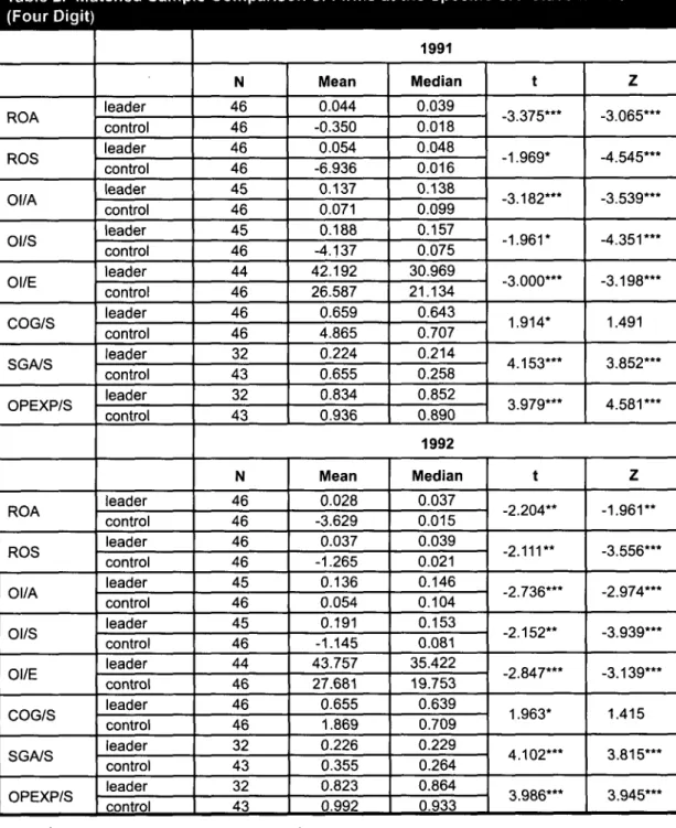
Tables 2 and 3 list the results of the matched sample procedures with benchmarks selected using the two and four digit SIC codes. The t-statistic from the t-test and the Z-t-statistic from the Wilcoxon test are reported. Following the
conven-tion in prior studies, a negative sign is included before the test statistic if the performance of the leader group is higher than the control group and vice versa. Hence, a significant negative test statistic in profit ratios and a significant positive test statistic for cost ratios will indicate superior IT capability effect.
We found strong support for both of our hypothe-ses, with profit ratios significantly higher for the leader sample and cost ratios significantly lower for the control sample, in most cases. The results show that, with a few exceptions, the pairwise t-test and Wilcoxon signed-ranks t-test indicate
Santhanam & Hartono/Unking iT Capabiiity to Firm Performance
Table 2. Matched Sample Comparison of Firms at the Specific SIC Classification
(Four Digit)
ROA ROS Ol/A Ol/S Ol/E COG/S SGA/S OPEXP/S ROA ROS Ol/A Ol/S Ol/E COG/S SGA/S OPEXP/S leader control leader control leader control leader control leader control leader control leader control leader control leader control leader control leader control leader control leader control leader control leader control leader control 1991 N 46 46 46 46 45 46 45 46 44 46 46 46 32 43 32 43 Mean 0.044 -0.350 0.054 -6.936 0.137 0.071 0.188 -4.137 42.192 26.587 0.659 4.865 0.224 0.655 0.834 0.936 Median 0.039 0.018 0.048 0.016 0.138 0.099 0.157 0.075 30.969 21.134 0.643 0.707 0.214 0.258 0.852 0.890 t -3.375*" -1.969* -3.182*" -1.961* -3.000*** 1.914* 4.153*" 3.979"* Z -3.065"* -4.545*** -3.539*" - 4 . 3 5 1 * " -3.198*" 1.491 3.852*" 4 . 5 8 1 * " 1992 N 46 46 46 46 45 46 45 46 44 46 46 46 32 43 32 43 Mean 0.028 -3.629 0.037 -1.265 0.136 0.054 0.191 -1.145 43.757 27.681 0.655 1.869 0.226 0.355 0.823 0.992 Median 0.037 0.015 0.039 0.021 0.146 0.104 0.153 0.081 35.422 19.753 0.639 0.709 0.229 0.264 0.864 0.933 t -2.204** -2.111" -2.736*" -2.152" -2.847*" 1.963* 4.102*" 3.986*" Z - 1 . 9 6 1 " -3.556*" -2.974*** -3.939*** -3.139*" 1.415 3.815*" 3.945***ROA: Return on Assets; ROS: Return on Sales; Ol/A: Operating Income to Assets; Ol/S: Operating Income to Saies; Oi/E: Operating Income to Employees; COG/S: Cost of Goods Sold to Sales; SGA/S: Selling and General Administration Expense to Saies; OPEXP/S: Operating Expenses to Saies
•Significant at the 10 percent ievei of significance. "Significant at the 5 percent ievel of significance. •"Significant at the 1 percent Ievei of significance.
Santhanam & Hartono/Linking IT Capability to Firm Performance
Table 2. Matched Sample Comparison of Firms at the Specific SIC Classification 1
(Four Digit) (Continued) |
ROA ROS Ol/A Ol/S Ol/E COG/S SGA/S OPEXP/S ROA ROS Ol/A Ol/S Ol/E COG/S SGA/S OPEXP/S leader control leader control leader control leader control leader control leader control leader control leader control leader control leader control leader control leader control leader control leader control leader control leader control 1993 N 45 46 45 46 43 46 43 46 42 46 45 46 32 43 32 43 Mean 0,034 -1.430 0.053 -0,780 0,141 0,076 0,213 -0,617 52.074 28,750 0,636 1,333 0,224 0,395 0,812 1,027 Median 0,035 0,019 0.049 0,027 0,148 0,099 0,168 0,085 35,563 20,456 0,624 0,711 0.232 0,253 0,841 0,933 t -2,832*** -2,253** -3,808*** -2,295** -3,896*** 1,947* 3,312*** 3,432*** Z -2,568*** -3,234*** -3,961*** -4,081*** -4.408*** 1,608 3,459*** 3,945*** 1994 N 45 46 45 46 44 46 44 46 40 46 45 46 31 43 31 43 Mean 0,055 -4.239 0,077 -2,149 0,143 0.036 0,217 -1,889 60,625 23,920 0,636 2,630 0,218 0.373 0,808 1,015 Median 0,048 0,010 0.064 0,030 0,147 0,094 0,182 0,079 46,369 21,613 0,671 0,703 0,223 0.261 0.838 0,930 t -3,167*** -1,996* -3,297*** -1,970* -4,235*** 1,863* 2,640** 2.935*** Z -3,177*** -3,516*** -3,875*** -4,481*** -4,409*** 1,597 3,723*** 4,488***
ROA: Return on Assets; ROS: Return on Sales; Ol/A: Operating Income to Assets; Ol/S: Operating Income to Sales; Ol/E: Operating Income to Employees; COG/S: Cost of Goods Sold to Sales; SGA/S: Selling and General Administration Expense to Sales; OPEXP/S: Operating Expenses to Sales
'Significant at the 10 percent level of significance, "Significant at the 5 percent level of significance, "'Significant at the 1 percent level of significance.
Sartthanam & Hartono/Unking IT Capability to Firm Performance
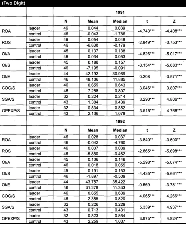
Table 3. Matched Sample Comparison of Firms at the Primary SIC Classification
(Two Digit)
ROA ROS Ol/A Ol/S Ol/E COG/S SGA/S OPEXP/S ROA ROS Ol/A Ol/S Ol/E COG/S SGA/S OPEXP/S leader control leader control leader control leader control leader control leader control leader control leader control leader control leader control leader control leader control leader control leader control leader control leader control 1991 N 46 46 46 46 45 46 45 46 44 46 46 46 32 43 32 43 Mean 0.044 -0.043 0.054 -6.838 0.137 0.034 0.188 -7.195 42.192 48.136 0.659 7.258 0.224 1.384 0.834 2.136 Median 0.039 -1.786 0.048 -0.179 0.138 0.053 0.157 -0.091 30.969 11.885 0.643 0.807 0.214 0.439 0.852 1.078 t -4.743*** -2.849*** -4.826*** -3.154*** 0.208 3.046*** 3.290*** 3.515*** Z -4.408*** -3.753*** -5.017*** -5.683*** -3.571*** 3.807*** 4.806*** 4.768*** 1992 N 46 46 46 46 45 46 45 46 44 46 46 46 32 43 32 43 Mean 0.028 -0.042 0.037 -5.880 0.136 0.018 0.191 -1.897 43.757 31.278 0.655 2.385 0.226 0.713 0.823 2.259 Median 0.037 -4.760 0.039 -0.462 0.146 0.055 0.153 -0.509 35.422 11.333 0.639 0.820 0.229 0.431 0.864 1.037 t -3.840** -2.865*** -5.298*** -4.435*** -0.669 4.065*** 5.339*** 3.875*** Z -3.600** -5.698*** -5.074*** -5.661*** -3.781*** 4.266*** 4.937*** 4.824***ROA: Return on Assets; ROS: Return on Sales; Ol/A: Operating Income to Assets; Ol/S: Operating Income to Sales; Ol/E: Operating Income to Employees; COG/S: Cost of Goods Sold to Sales; SG/WS: Selling and General Administration Expense to Sales; OPEXP/S: Operating Expenses to Sales
"Significant at the 10 percent level of significance. "Significant at the 5 percent level of significance. •"Significant at the 1 percent level of significance.
Santhanam & Hartono/Unking IT Capabiiity to Firm Performance
Table 3. Matched Sample Comparison of Firms at the Primary SIC Classification
(Two Digit) (Continued)
ROA ROS Ol/A Ol/S Ol/E COG/S SGA/S OPEXP/S ROA ROS Ol/A Ol/S Ol/E COG/S SGA/S OPEXP/S leader control leader control leader control leader control leader control leader control leader control leader control leader control leader control leader control leader control leader control leader control leader control leader control 1993 N 45 46 45 46 43 46 43 46 42 46 45 46 32 43 32 43 Mean 0.034 0.731 0.053 -2.059 0.141 -0.329 0.213 -1.874 52.074 35.366 0.636 2.346 0.224 0.680 0.812 1.444 Median 0.035 -1.749 0.049 -0.240 0.148 0.054 0.168 0.032 35.563 12.986 0.624 0.798 0.232 0.385 0.841 1.077 t 1.193 -4.066*** -1.996* -4.112*** -1.143 3.481*** 5.753*** 5.041*** Z -3.889*** -5.085*** -5.132*** -5.422*** -4.333*** 3.877*** 4.693*** 4.824*** 1994 N 45 46 45 46 44 46 44 46 40 46 45 46 31 43 31 43 Mean 0.055 -0.170 0.077 -2.573 0.143 -4.020 0.217 -1.853 60.625 37.873 0.636 2.514 0.218 0.485 0.808 1.126 Median 0.048 -9.398 0.064 -0.161 0.147 0.062 0.182 0.015 46.369 13.326 0.671 0.776 0.223 0.479 0.838 1.116 t -3.954*** -3.123*** -4.537*** -3.131*** -1.779* 2.863*** 6.738*** 6.913*** Z -4.532*** -5.096*** -5.147*** -5.240*** -4.503*** 2.760*** 4.507*** 4.723***
ROA: Return on Assets; ROS: Return on Sales; Ol/A: Operating Income to Assets; Ol/S: Operating income to Saies; Oi/E: Operating income to Empioyees; COG/S: Cost of Goods Sold to Saies; SGA/S: Seiiing and Generai Administration Expense to Saies; OPEXP/S: Operating Expenses to Saies
"Significant at the 10 percent ievel of significance. "Significant at the 5 percent ievel of significance. •"Significant at the 1 percent Ievei of significance.
Santhanam & Hartono/Unking IT Capability to Firm Performance
similar results. From Tables 2 and 3, it is seen that, in each of the four years, for industry aver-ages computed using both two and four digit SIC codes, for all profit ratios and three of the cost ratios, the average performance of the leaders was significantly better than the industry aver-ages. These results are not only consistent with the results found earlier, but in some cases, stronger. For instance, the SGA/S ratio was signi-ficantly lower for the leader sample only in one year in the earlier study, but in this study, it was lower in all four years. In addition, the level of significance of the effects was also higher in several cases (for example tests of Ol/E in 1991 in Table 2, Ol/A in 1991 in Table 3, and OPEXP/S in 1991 in Tables 2 and 3).
Note that while not significant, in two instances, the t-tests indicated results that were contrary to expectations. The mean of ROA in 1993 and Ol/E in 1991 (Table 3) were found to be lower for the leader sample instead of being higher. The Wilcoxon test indicated that the value of the median was significantly higher for both the ratios. Considering that 64 different tests were per-formed, it is not unreasonable to observe a few inconsistencies that might have occurred by chance.
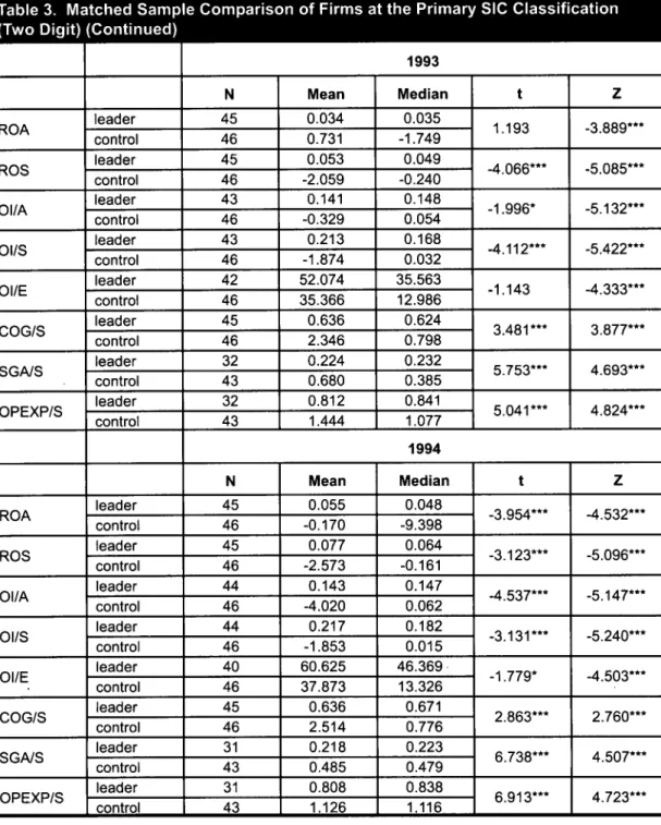
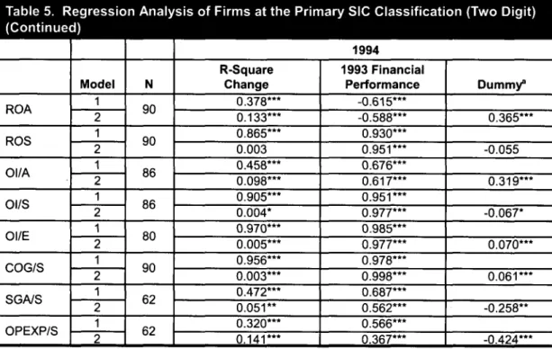
As seen in Tables 4 and 5, there is variation in the magnitude and levels of significance depending on the year of analysis and whether control firms were matched at the four digit or two digit SIC code level. When control firms at the four digit level were used (Table 4), only 3 of the 24 per-formance measures were found to be significant. When control firms are matched at the two digit level (Table 5), 16 of the 24 performance mea-sures were found to be significant. Table 4 shows that in 1992, when industry averages based on the four digit SIC code are used, no significant effects are observed on any of the performance measures. However, from Table 5 it is seen that for the same year, when industry averages based on the two digit SIC code are used, significant effects are observed on all performance mea-sures. On six ofthe eight ratios (ROS, Ol/S, Ol/E, COG/S, SGA/S, and OPEXP/S), the effects ofthe IT capability factor were highly significant (p < 0.01). It should also be noted that" on two ratios in Table 4 (ROA (1993) and Ol/S (1994)), and two ratios in Table 5 (Ol/S (1994) COG/S (1994)), the coefficient of the binary variable was significant but not in the expected direction. Thus, the results for hypotheses 3 and 4 seem to depend on the benchmark firms used for comparison and are less pronounced than that obtained by using the matched sample comparison procedure.
Adjusting for Prior Financial
Performance (Hypothesis 3
and 4)
Tables 4 and 5 show the results of the regression analysis that seek to examine the effects of IT capability after adjusting for prior year's firm per-formance. Changes in R-square and the regres-sion coefficients of models described in equations (1) and (2) are shown. It is important to note from the results shown for model 1 that, in almost all cases, prior performance has a significant effect on current year's performance. In analyzing IT capability effect, a significant positive coefficient for the dummy term relating to profit ratios and a significant negative coefficient for the dummy term relating to cost ratios would indicate an IT capability effect on performance.
Testing for Sustained Effects
of IT Capability
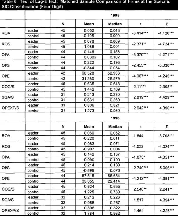
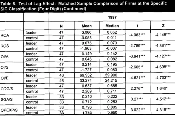
Matched Sample Comparison Procedure for Sustained Effects (Hypotheses 5 and 6) Tables 6 and 7 present the results of matched sample comparison procedures with control firms at the four digit SIC and the two digit SIC code respectively. The results indicate that the profit ratios are significantly higher and the cost ratios are significantly lower for IT leaders, when com-pared to the industry averages in all cases when the Wilcoxon test is used and in almost all cases when the t-test is used. The few exceptions were t-test performed on one profit ratio for three years (Ol/E 1995,1996,1997 in Table 7) and four ratios
Santhanam & Hartono/Unking IT Capability to Firm Performance
Table 4. Regression Analysis of Firms at the Specific SIC Classification (Four Digit)
ROA ROS Ol/A Ol/S Ol/E COG/S SGA/S OPEXP/S ROA ROS Ol/A Ol/S Ol/E COG/S SGA/S OPEXP/S Model 1 2 1 2 1 2 1 2 1 2 1 2 1 2 1 2 Model 1 2 1 2 1 2 1 2 1 2 1 2 1 2 1 2 N 92 92 90 90 88 92 64 64 N 91 90 86 86 84 90 64 64 1992 R-Square Change 0.247*** 0.005 0.518*** 0.004 0.389*** 0.007 0.937*** 0.000 0.941*** 0.000 0.975*** 0.000 0.740*** 0.000 0.642*** 0.001 1991 Financial Performance 0.497*** 0.471*** 0.720*** 0.707*** 0.624*** 0.593*** 0.987*** 0.985*** 0.970*** 0.971*** 0.987*** 0.987*** 0.860*** 0.847*** 0.801*** 0.789*** Dummy° 0.074 0.061 0.089 0.007 -0.004 0.000 -0.039 -0.027 1993 R-Square Change 0.642*** 0.011* 0.999*** 0.000 0.518*** 0.310** 0.998*** 0.000 0.973*** 0.001 0.997*** 0.000 0.946*** 0.000 0.911*** 0.000 1992 Financial Performance 0.801*** 0.774*** 1.000*** 0.999*** 0.720*** 0.661*** 0.999*** 0.998*** 0.986*** 0.980*** 0.999*** 0.998*** 0.972*** 0.977*** 0.955*** 0.950*** Dummy° 0.109* 0.002 0.185** 0.007 0.026 -0.003 0.015 -0.011
Model 1: (Performance measure for year t) = f(Performance measure for year t-1)
Model 2: (Performance measure for year t) = f(Performance measure for year t-1, dummy: 1 = leader finn, 0 = control finn) 'Please note that for model 1, the dummy variable is not included and hence has no coefficient.
ROA: Return on Assets; ROS: Return on Sales; Ol/A: Operating Income to Assets; Ol/S: Operating Income to Sales; Ol/E: Income to Employees; COG/S: Cost of Goods Sold to Sales; SGA/S: Selling and General Administration Expense to Sales; Operating Expenses to Sales
"Significant at the 10 percent level of significance. "Significant at the 5 percent level of significance. ""Significant at the 1 percent level of significance.
Operating OPEXP/S:
Santhanam & Hartono/Linking IT Capability to Firm Performance
Table 4. Regression Analysis of Firms at the Specific SIC Classificat
(Continued)
ROA ROS Ol/A Ol/S Ol/E COG/S SGA/S OPEXP/S Model 1 2 1 2 1 2 1 2 1 2 1 2 1 2 1 2 N 90 90 86 86 . 80 90 62 63on (Four Digit)
1994 R-Square Change 0,680*** 0,009* 0,994*** 0,000 0,787*** 0,000 0,993*** 0.0001* 0,623*** 0,027** 0.992*** 0,000 0,625*** 0,001 0,661*** 0.000 1993 Financial Performance 0.825*** 0,794*** 0,997*** 0,999*** 0,887*** 0,878*** 0.996*** 1,000*** 0,790*** 0,744*** 0,996*** 0,999*** 0,790*** 0,778*** 0,813*** 0,813*** Dummy° 0,101* -0,009 0,023 -0,017* 0,170** 0,013 -0,040 -0,001Model V, (Performance measure for year t) = f(Pertorniance measure for year t-1)
Model,2: (Performance measure for year t) = f(Perfomiance measure for year t-1, dummy: 1 = leader firm, 0 = control firm) 'Please note that for model 1, the dummy variable is not included and hence has no coefficient,
ROA: Retum on Assets; ROS: Return on Sales; Ol/A: Operating Income to Assets; Ol/S: Operating Income to Sales; Ol/E: Operating Income to Employees; COG/S: Cost of Goods Sold to Sales; SGA/S: Selling and General Administration Expense to Sales; OPEXP/S: Operating Expenses to Sales
"Significant at the 10 percent level of significance, "Significant at the 5 percent ievel of significance. '"Significant at the 1 percent level of significance.
Santhanam & Hartono/Unking IT Capability to Firm Performance
1 Table 5. Regression Analysis of Firms at the Primary SIC Classification (Two Digit)
ROA ROS Ol/A Ol/S Ol/E COG/S SGA/S OPEXP/S ROA ROS Ol/A Ol/S Ol/E COG/S SGA/S OPEXP/S Model 1 2 1 2 1 2 1 2 1 2 1 2 1 2 1 2 Model 1 2 1 2 1 2 1 2 1 2 1 2 1 2 1 2 N 92 92 90 90 88 92 64 64 N 90 90 86 86 84 90 64 64 1992 R-Square Change 0.043** 0.064** 0.008 0.106*** 0.952*** 0.002* 0.394*** 0.050*** 0.954*** 0.007*** 0.336*** 0.052*** 0.920*** 0.018*** 0.084** 0.117*** 1991 Financial
Performance
0.206** 0.064 -0.092 -0.190* 0.976*** 0.952*** 0.628*** 0.551*** 0.977*** 0.978*** 0.580*** 0.506*** 0.959*** 0.906*** 0.290* 0.142 Dummy° 0.290** 0.340*** 0.050* 0.236*** 0.083*** -0.240*** -0.144*** -0.373*** 1993 R-Square Change 0.028 0.000 0.019 0.122*** 0.178*** 0.002 0.692*** 0.001 0.951*** 0.001 0.719*** 0.000 0.239*** 0.077*** 0.000 0.253*** 1992 FinancialPerformance
-0.166 -0.160 0.137 0.031 0.422*** 0.452*** 0.832*** 0.816*** 0.975*** 0.973*** 0.848*** 0.848*** 0.489*** 0.338*** 0.011 -0.228* Dummy° -0.021 0.365*** -0.055 0.037 0.029 0.000 -0.315*** -0 557***Model 1: (Performance measure for year t) = f(Perforniance measure for year t-1)
Model 2: (Performance measure for year t) = f(Performance measure for year t-1, dummy: 1 = leader firm, 0 = control finn) 'Please note that for model 1, the dummy variable is not included and hence has no coefficient.
ROA: Return on Assets; ROS: Return on Sales; Ol/A: Operating Income to Assets; Ol/S: Operating Income to Sales; Ol/E: Income to Employees; COG/S: Cost of Goods Sold to Sales; SGA/S: Selling and General Administration Expense to Sales; Operating Expenses to Saies
"Significant at the 10 percent level of significance. "Significant at the 5 percent levei of significance. •"Significant at the 1 percent ievel of significance.
Operating OPEXP/S:
Santtianam & Hartono/Linidng iT Capabiiity to Firm Performance
Table 5. Regression Analysis of Firms at the Primary SIC Classification (Two Digit)
(Continued)
ROA ROS Ol/A OI/S Ol/E COG/S SGA/S OPEXP/S Model 1 2 1 2 1 2 1 2 1 2 1 2 1 2 1 2 N 90 90 86 86 80 90 62 62 1994 R-Square Change 0.378*** 0.133*** 0.865*** 0.003 0.458*** 0.098*** 0.905*** 0.004* 0.970*** 0.005*** 0.956*** 0.003*** 0.472*** 0.051** 0.320*** 0.141*** 1993 Financial Performance -0.615*** -0.588*** 0.930*** 0.951*** 0.676*** 0.617*** 0.951*** 0.977*** 0.985*** 0.977*** 0.978*** 0.998*** 0.687*** 0.562*** 0.566*** 0.367*** Dummy° 0.365*** -0.055 0.319*** -0.067* 0.070*** 0.061*** -0.258** -0.424***Model 1: (Performance measure for year t) = f(Performance measure for year t-1)
Model 2: (Performance measure for year t) = f(Performance measure for year t-1, dummy: 1 = leader firm, 0 = control firm) 'Please note that for model 1, the dummy variable is not included and hence has no coefficient.
ROA: Return on Assets; ROS: Return on Sales; Ol/A: Operating Income to Assets; OI/S: Operating Income to Sales; Ol/E: Income to Employees; COG/S: Cost of Goods Sold to Sales; SGA/S: Selling and General Administration Expense to Sales; Operating Expenses to Sales
'Significant at the 10 percent level of significance. "Significant at the 5 percent level of significance. •"Significant at the 1 percent level of significance.
Operating OPEXP/S:
Santhanam & Hartono/Unking IT Capability to Firm Performance
Table 6. Test of Lag-Effect: Matched Sample Comparison of Firms at the Specific
SIC Classification (Four Digit)
ROA ROS Ol/A Ol/S Ol/E COG/S SGA/S OPEXP/S ROA ROS Ol/A Ol/S Ol/E COG/S SGA/S OPEXP/S leader control leader control leader control leader control leader control leader control leader control leader control leader control leader control leader control leader control leader control leader control leader control leader control 1995 N 45 45 45 45 44 44 44 44 42 42 45 45 31 31 31 31 Mean 0.052 -0.105 0.078 -1.088 0.146 0.0002 0.222 -0.844 66.528 31.380 0.635 1.442 0.213 0.631 0.806 1.273 Median 0.043 0.009 0.069 -0.004 0.153 0.102 0.193 0.054 52.933 26.579 0.648 0.709 0.230 0.260 0.821 0.950 t -3.414*** -2.371** -3.370*** -2.453** -4.067*** 2.111** 2.819*** 2.942*** Z -4.120*** -4.724*** -4.271*** -5.030*** -4.245*** 2.308** 4.429*** 4.390*** 1996 N 45 45 45 45 45 45 45 45 44 44 45 45 32 32 32 32 Mean 0.060 -0.220 0.083 -0.907 0.142 -0.090 0.214 -0.898 67.515 33.055 0.634 1.225 0.212 0.958 0.806 1.784 Median 0.052 0.011 0.071 0.004 0.137 0.100 0.189 0.076 56.654 22.414 0.655 0.739 0.226 0.257 0.822 0.932 t -1.644 -1.532 -1.873* -2.740*** -4.212*** 2.546** 1.517 1.464 Z -3.708*** -4.024*** -4.351*** -5.006*** -4.691*** 2.241** 4.394*** 4.226***
ROA: Retum on Assets; ROS: Retum on Sales; Ol/A: Operating Income to Assets; Ol/S: Operating income to Saies; Oi/E: Operating income to Empioyees; COG/S: Oost of Goods Soid to Saies; SGA/S: Seiling and General Administration Expense to Saies; OPEXP/S: Operating Expenses to Sales
'Significant at the 10 percent Ievei of significance. "Significant at the 5 percent ievei of significance. '"Significant at the 1 percent ievei of significance.
Santhanam & Hartono/Unking iT Capabiiity to Firm Performance
Table 6. Test of Lag-Effect: Matched Sample Comparison of Firms at the Specific
SIC Classification (Four Digit) (Continued)
ROA ROS Ol/A OI/S Ol/E COG/S SGA/S OPEXP/S leader control leader control leader control leader control leader control leader control leader control leader control 1997 N 47 47 47 47 47 47 47 47 46 46 47 47 33 33 33 33 Mean 0.060 -0.053 0.075 -1.963 0.149 0.046 0.214 -1.727 69.932 33.274 0.637 2.289 0.210 0.712 0.796 1.383 Median 0.052 0.011 0.073 -0.007 0.142 0.082 0.195 0.083 59.900 24.215 0.685 0.711 0.222 0.253 0.805 0.950 t -4.083*** -2.789*** -3.941*** -2.605** -4.621*** 2.276** 3.27*** 3.022*** Z -4.148*** -4.381*** -4.127*** -4.698*** -4.703*** 1.640* 4.512*** 4.315***
ROA: Return on Assets; ROS: Return on Sales; Ol/A: Operating Income to Assets; OI/S: Operating Income to Sales; Ol/E; Operating Income to Employees; COG/S: Cost of Goods Sold to Sales; SGA/S; Selling and General Administration Expense to Sales; OPEXP/S; Operating Expenses to Sales
•Significant at the 10 percent level of significance. "Significant at the 5 percent level of significance. •"Significant at the 1 percent level of significance.
Santhanam & i-iartono/Lini<ing iT Capability to Firm Performance
Table 7. Test of Lag-Effect: Matched Sample Comparison of Firms at the Primary
SIC Classification (Two Digit)
ROA ROS Ol/A Ol/S Ol/E COG/S SGA/S OPEXP/S ROA ROS Ol/A Ol/S Ol/E COG/S SGA/S OPEXP/S leader control leader control leader control leader control leader control leader control leader control leader control leader control leader control leader control leader control leader control leader control leader control leader control 1995 N 45 45 45 45 44 44 44 44 42 42 45 45 31 31 31 31 Mean 0.052 -0.143 0.078 -2.152 0.146 -0.041 0.222 -1.862 66.528 48.455 0.635 2.401 0.213 0.661 0.806 1.295 Median 0.043 -0.042 0.069 -0.188 0.153 0.042 0.194 0.024 52.933 17.376 0.648 0.779 0.230 0.421 0.821 1.044 t -3.980*** -3.155*** -4.544*** -3.083*** -0.715 2.806*** 4.673*** 4.761*** Z -4.724*** -5.322*** -5.252*** -5.345*** -4.232*** 3.471*** 4.429*** 4.723*** 1996 N 45 45 45 45 45 45 45 45 44 44 45 45 32 32 32 32 Mean 0.060 -0.164 0.083 -4.494 0.142 -0.042 0.214 -3.863 67.515 62.463 0.634 4.299 0.212 0.775 0.806 1.509 Median 0.052 -0.087 0.071 -0.299 0.137 0.006 0.189 -0.009 56.654 14.286 0.655 0.805 0.226 0.488 0.822 1.112 t -3.466*** -4.219*** -4.194*** -3.792*** -0.184 3.450*** 2.719*** 2.508** Z -5.514*** -5.435*** -5.322*** -5.198*** -3.373*** 3.618*** 4.263*** 4.675***
ROA: Return on Assets; ROS: Return on Sales; Ol/A: Operating Income to Assets; Ol/S: Operating Income to Sales; Ol/E: Operating Income to Employees; COG/S: Cost of Goods Sold to Sales; SGA/S: Selling and General Administration Expense to Sales; OPEXP/S: Operating Expenses to Sales
"Significant at the 10 percent ievel of significance. "Significant at the 5 percent ievei of significance. ""Significant at the 1 percent ievel of significance.
Santhanam & Hartono/Linidng IT Capabiiity to Firm Performance
Table 7. Test of Lag-Effect: Matched Sample Comparison of Firms at the Primary
SIC Classification (Two Digit) (Continued)
ROA ROS Ol/A OI/S Ol/E COG/S SGA/S OPEXP/S leader control leader control leader control leader control leader control leader control leader control leader control 1997 N 47 47 47 47 47 47 47 47 46 46 47 47 33 33 33 33 Mean 0.060 -0.130 0.075 -3.616 -0.149 -0.020 0.214 -3.143 69.932 57.954 0.637 3.282 0.210 1.471 0.796 2.221 Median 0.052 -0.025 0.073 -0.272 0.142 0.025 0.195 -0.210 59.900 18.441 0.685 0.805 0.222 0.584 0.805 1 335 t -5.619*** -3.883*** -5.378*** -3.716*** -0.469 3.259*** 4.689*** 4.792*** Z -5.704*** -5.333*** -5.376*** -5.323*** 3.644*** 3.513*** 4.619*** 4.780***
ROA: Return on Assets; ROS: Return on Sales; Ol/A: Operating Income to Assets; OI/S: Operating Income to Sales; Ol/E: Operating Income to Employees; COG/S: Cost of Goods Sold to Sales; SGA/S: Selling and General Administration Expense to Sales; OPEXP/S: Operating Expenses to Sales
'Significant at the 10 percent level of significance. "Significant at the 5 percent level of significance. •"Significant at the 1 percent level of significance.
in 1996 (ROA, ROS, SGA/S, and OPEXP/S in Table 6), whose differences are in the correct direction but are not significant.
Regression Analysis Procedure for Sustained Effects (Hypothesis 7 and 8)
The effects of the regression analysis testing for sustained effects of IT capability are shown in Tables 8 and 9. When industry averages based on four digit SIC code are used, 12 of 24 ratios indicate significantly better financial performance by leaders during the three years after they were rated (Table 8). These effects are most pro-nounced in the third year (i.e., 1997) where signifi-cant effects are observed for six of the eight per-formance ratios. The results with industry
aver-ages based on the two digit SIC code shown in Table 9 indicate stronger effects for leaders with 20 of 24 ratios being significant. Once again, in the third year after being identified as leaders, the results are strong with seven of the eight ratios being significant. In one ratio (Ol/E 1995 in Table 9) the results were not in the expected direction.
Similar to the results observed for current effects of IT capability, the analysis for sustained effects also showed some variability depending on the benchmark firms used for comparison. In both cases, the results are generally stronger when control firms are matched with leaders at the two digit level. However, when current effects of IT capability were analyzed, the results were considerably stronger at the two digit level and
Santhanam & i-iartono/Lini<ing iT Capabiiity to Firm Performance
Table 8. Test of Lag-Effect: Regression Analysis at the Specific SIC Classification
(Four Digit)
ROA ROS Ol/A OI/S Ol/E COG/S SGA/S OPEXP/S ROA ROS Ol/A OI/S Ol/E COG/S SGA/S OPEXP/S Model 1 2 1 2 1 2 1 2 1 2 1 2 1 2 1 2 Model 1 2 1 2 1 2 1 2 1 2 1 2 1 2 1 2 N 94 94 93 93 89 94 77 77 N 94 94 93 93 91 94 77 77 1995 R-Square Change 0.780*** 0.004 0.939*** 0.003** 0.737*** 0.008 0.928*** 0.005** 0.739*** 0.000 0.935*** 0.001 0.658*** 0.013* 0.551*** 0.019* 1994 Financiai Performance 0.883*** 0.859*** 0.969*** 0.958*** 0.859*** 0.831*** 0.963*** 0.950*** 0.860*** 0.853*** 0.967*** 0.960*** 0.811*** 0.783*** 0.742*** 0.698*** Dummy" 0.070 0.058** 0.080 0.069** 0.022 -0.037 -0.118* -0.144* 1996 R-Square Change 0.019 0.017 0.117*** 0.011 0.040* 0.017 0.231*** 0.030* 0.828*** 0.003 0.761*** 0.009* 0.080** 0.014 0.084** 0.011 1995 Financial Performance 0.136 0.085 0.343*** 0.316*** 0.199* 0.148 0.480*** 0.435*** 0.910*** 0.925*** 0.837*** 0.852*** 0.284** 0.245** 0.290*** 0.251** Dummy" 0.141 0.110 0.139 0.179* -0.060 -0.095* -0.126 -0.111Model 1: (Performance measure for year t) = f(Performance measure for year t-1)
Model 2; (Performance measure for year t) = fjPerformance measure for year t-1, dummy: 1 = leader firm, 0 = control firm) 'Please note that for model 1, the dummy variable is not included and hence has no coefficient.
ROA: Retum on Assets; ROS: Return on Sales; Ol/A: Operating Income to Assets; OI/S: Operating Income to Sales; Ol/E: Operating Income to Employees; COG/S: Cost of Goods Sold to Sales; SGA/S: Selling and General Administration Expense to Sales; OPEXP/S: Operating Expenses to Sales
"Significant at the 10 percent level of significance. "Significant at the 5 percent level of significance. •"Significant at the 1 percent level of significance.
Santhanam & i-lartono/Lini<ing iT Capabiiity to Firm Performance
Table 8. Test of Lag-Effect: Regression Analysis at the Specific SIC Classification (Four Digit) (Continued)
ROA ROS Ol/A Ol/S Ol/E COG/S SGA/S OPEXP/S Model 1 2 1 2 1 2 1 2 1 2 1 2 1 2 1 2 N 94 94 94 94 93 94 78 78 1997 R-Square Change 0.032* 0.152*" 0.037* 0.066** 0.055** 0.137*" 0.199*" 0.022 0.945*" 0.004" 0.702*" 0.000 0.008 0 . 0 6 1 " 0.004 0 . 0 7 1 " 1996 Financiai Performance 0.180* 0.112 0.191* 0.143 0.235** 0.162* 0.446*** 0.402*" 0.972*** 0.962*" 0.838"* 0.840*" 0.087 0.035 0.065 0.010 Dummy^ 0.396*" 0 . 2 6 1 " 0.377*" 0.154 0.062" 0.007 -0.253" -0.272"
Model 1: (Performance measure for year I) = f(Performance measure for year t-1)
Model 2: (Performance measure for year t) = f(Performance measure for year t-1, dummy: 1 = leader firm, 0 = control firm) 'Please note that for model 1, the dummy variable is not included and hence has no coefficient.
ROA: Retum on Assets; ROS: Return on Sales; Ol/A: Operating Income to Assets; Ol/S: Operating Income to Sales; Ol/E: Income to Employees; COG/S: Cost of Goods Sold to Sales; SGA/S: Selling and General Administration Expense to Sales; Operating Expenses to Sales
•Significant at the 10 percent level of significance. "Significant at the 5 percent level of significance. •"Significant at the 1 percent level of significance.
Operating OPEXP/S:
Santhanam & Hartono/Linking IT Capability to Firm Performance
Table 9. Test of Lag-Effect: Regression Analysis of Firms at the Primary SIC
Classification (Two Digit)
ROA ROS Ol/A Ol/S Ol/E COG/S SGA/S OPEXP/S ROA ROS Ol/A Ol/S Ol/E COG/S SGA/S OPEXP/S Model 1 2 1 2 1 2 1 2 1 2 1 2 1 2 1 2 Model 1 2 1 2 1 2 1 2 1 2 1 2 1 2 1 2 N 94 94 93 93 89 94 80 80 N 94 94 93 93 91 94 80 80 1995 R-Square Change 0.909*** 0.001 0.990*** 0.001** 0.961*** 0,001* 0,996*** 0.001*** 0.948*** 0.005*** 0,997*** 0,001** 0.498*** 0,018* 0,427*** 0,036** 1994 Financial Performance 0.953*** 0,942*** 0,995*** 0.988*** 0,980*** 0,963*** 0,998*** 0.992*** 0,974*** 0,984*** 0.998*** 0.994*** 0,706*** 0,640*** 0.653*** 0,541*** Dummy" 0,027 0,025** 0,040* 0,019*** -0,071*** -0,015** -0.148* -0,221** 1996 R-Square Change 0.243*** 0,028* 0,215*** 0,077*** 0.410*** 0.020* 0,120*** 0,078*** 0,967*** 0.001* 0.096*** 0,069*** 0,175*** 0,009 0,135*** 0.009 1995 Financial Performance 0,493*** 0,418*** 0.464*** 0.369*** 0,640*** 0,569*** 0,346*** 0.254** 0,983*** 0,985*** 0,310*** 0.229** 0.418*** 0.372*** 0,368*** 0.315** Dummy" 0,183* 0.293*** 0,159* 0,293*** -0,037* -0,274*** -0,105 -0,107
Model 1: (Performance measure for year t) = f(Performance measure for year t-1)
Model 2: (Performance measure for year t) = fjPerformance measure for year t-1, dummy: 1 = leader firm, 0 = control firm) 'Please note that for model 1, the dummy variable is not included and hence has no coefficient,
ROA: Return on Assets; ROS: Return on Sales; Ol/A: Operating Income to Assets; Ol/S: Operating Income to Sales; Ol/E: Income to Employees; COG/S; Cost of Goods Sold to Sales; SGA/S: Selling and General Administration Expense to Sales; Operating Expenses to Sales
"Significant at the 10 percent level of significance. "Significant at the 5 percent level of significance. '"Significant at the 1 percent level of significance.
Operating OPEXP/S:
Santhanam & i-iartono/Linidng iT Capabiiity to Firm Performance
Table 9. Test of Lag-Effect: Regression Analysis of Firms at the Primary SIC
Classification (Two Digit) (Continued)
ROA ROS Ol/A Ol/S Ol/E COG/S SGA/S OPEXP/S Model 1 2 1 2 1 2 1 2 1 2 1 2 1 2 1 2 N 94 94 94 94 93 94 81 81 1997 R-Square Change 0.128*" 0.190*" 0.390*** 0.017 0.316" 0.095*" 0.245*" 0.037" 0.988*** 0 . 0 0 1 " 0.232"* 0.031* 0.043* 0.136*" 0.041* 0.150*" 1996 Financial Performance 0.358"* 0.193" 0.624"* 0.565"* 0.562*" 0.423"* 0.495*** 0.417*" 0.994"* 0.994*** 0.482*" 0.418*" 0.208* 0.104 0.202* 0.095 Dummy^ 0.466*" 0.143 0.338*" 0.207" 0.027" -0.187* -0.383*" -0.402*"
Model 1: (Perfonnance measure for year t) = f(Performance measure for year t-1)
Model 2: (Performance measure for year \) = f(Performance measure for year t-1, dummy: 1 = leader firm, 0 = control firm)
'Please note that for model 1, the dummy variable is not included and hence has no coefficient.
ROA: Retum on Assets; ROS: Return on Sales; Ol/A: Operating Income to Assets; Ol/S: Operating Income to Sales; Ol/E: Operating Income to Employees; COG/S: Cost of Goods Sold to Sales; SG/VS: Selling and General Administration Expense to Sales; OPEXP/S: Operating Expenses to Sales
•Significant at the 10 percent level of significance. "Significant at the 5 percent level of significance. •"Significant at the 1 percent level of significance.
markedly different from the results obtained at the four digit level. By contrast, for sustained effects, strong support for superior financial performance of leaders is observed at both the two and four digit SIC codes. These results suggest that in subsequent years, there is stronger evidence of a link between leaders and their financial perfor-mance. In addition, it is to be noted that the over-all results for IT capability obtained by combining the matched sample and regression analysis procedure were much stronger for sustained effects than for current effects.
Discussion
Berthon et al. (2002), Rosenthal (1991), and Tsang and Kwan (1999), among others, state that a theory development and knowledge creation process must consist of replications, extensions, and generalizations that provide new insights and add to the existing stock of knowledge. Aggre-gating the results of the various analyses con-ducted in this study provides information to build such cumulative knowledge. We frame the dis-cussion of the results into two categories: results
Santhanam & Hartono/Unking IT Capability to Firm Performance
that are consistent with those observed by Bharadwaj (2000), and others that while suppor-tive of prior results, provide a source of further insight.
When we conducted an empirical generalization test by utilizing the same matched sample proce-dures as in the prior study, the results indicated that IT capability effects on firm performance were very significant and similar to the results obtained earlier. It did not matter whether the benchmark firms were chosen on industry groupings matched with the leaders at the two or four digit SIC code. These results indicate that the RBV framework is robust. In addition, we examined whether there is evidence to suggest that IT capability has a sus-tained impact on firm performance. This aspect was not examined earlier and represents a con-ceptual extension of the prior study. We found strong evidence to suggest (both from the matched group and the regression analysis proce-dures) that IT capability does indeed have a sus-tained impact on firm performance. We observed that, in many cases, the relationship between IT capability and financial performance was stronger in later time periods than in the current time period. These results are consistent with RBV, which suggests that returns should be maximized over several time periods. Thus, these results verify (using different benchmarks) and extend (sustained financial performance) the findings observed earlier. Equally interesting are other results that provide support for prior findings but highlight important issues that must be addressed.
One key difference between this study and the prior study is that we used a different, more conservative analytical procedure, namely regres-sion analysis. When analyzed in this manner, the effects for IT capability were mixed and less pronounced. One possible explanation from a statistical perspective could be that the matched sample test is more powerful. Other alternative explanations can be examined from a theory development perspective. Such an examination facilitates the development of a more compre-hensive model and a refinement of the structures for using the underlying framework (Tsang and Kwang 1999),
Prior Financial Performance
In the regression analysis, the effect of prior financial performance was adjusted both on cur-rent financial performance (dependent variable) and the IT leader rating (independent variable). When analyzed in this manner, the effect of IT capability was less pronounced than that obtained via matched sample procedures. Our results indi-cate that there is a relationship between past and current financial performance. Further, the less pronounced results may have occurred because of a relationship between prior financial perfor-mance and the IT capability rating. Because of this halo effect, it becomes quite difficult to com-pletely isolate the effects of IT capability on current financial performance. From these results, it is clear that prior financial performance has to be acknowledged and adjusted using procedures similar to those utilized in this study. However, it is to be noted that there exists no perfect metho-dological solution exists to remove the halo effects of prior financial performance on leader ratings.
Benchmark Firms for Comparison
Another major difference we observed when utilizing the regression analysis procedures was that the significance of the results seemed to vary with the choice of benchmark firms. Unlike the matched sample procedures where variation in the benchmark firms did not matter, the results from the regression analysis indicated stronger effects when firms were matched at the two digit SIC code. Benchmark firms selected by matching leader firms at the two digit SIC code include a larger number of firms than those selected by matching at the four digit SIC code. Hence, having a larger sample of firms could have pro-vided a better approximation of the true mean (average performance) of the control firms. From a statistical perspective, this might be one explanation for the stronger effects observed using the two digit SIC code. One could also theorize that IT capabilities provide a much stronger performance differential in a hetero-geneous group of firms (formed using the two digit SIC code). However, in a relatively homogenous
Santhanam & Hartono/Unking IT Capabiiity to Firm Performance
group of firms (formed using the four digit SIC code), performance differentials could perhaps accrue due to other higher order capabilities (Teece et al. 1997). The effects of these higher order capabilities (such as those resulting from the complementary integration between IT and business capabilities) need to be examined. Thus, these differences in the effects of IT capa-bilities among the two sets of benchmark firms highlight the need for conducting more finely grained investigations of higher-order capabilities and the effects of various capability-building processes in organizations. It is also evident that the industry grouping or benchmark firms used in comparing financial performances are important in analyzing IT capability effects and close attention must be paid to this issue in future studies.
Identification of IT Leaders
It is important to note that the need for selecting appropriate benchmark firms arises because of the existing definitions and measures of IT leaders. Leaders were selected by industry experts based on their opinion of the firm's IT capability. This method of selecting leaders did not ask experts to rank each firm in the industry but asked them to identify those firms that they perceived to have superior IT capability compared to other firms in the industry. Note that this proxy method of identification of firms with superior IT capability does not provide a true multidimen-sional measure of a firm's capability as described by the RBV. Instead, the measurement and selection is binary with some firms being identified as leaders and others not. This leads to the prob-lem of identifying an appropriate set of benchmark firms whose financial performance can be compared to the leaders in order to evaluate the effects of superior IT capability.
In addition to the problem of identifying bench-mark firms, the binary nature of the leader mea-sure prevents researchers from directly comparing firm performance to their level of IT capability. In fact, further developments in the application of the RBV framework can be meaningful only if all of the firms in the industry can be examined. From
a methodological perspective, such investigations would be a substantive improvement over existing studies because this could allow researchers to investigate a larger set of firms in different indus-tries. More importantly, it could help in examining more finely grained relationships between IT capability and firm performance by evaluating the impact of incremental improvements in IT capa-bility on firm performance. The existing methods of identifying leaders and others do not allow for such research investigations to be conducted.
Longitudinal Studies
The binary nature of the assessment of IT capa-bility creates another difficulty in pursuing investigations using RBV. In this study, we found evidence of sustained impact, which suggests that in subsequent years, the financial performance of leaders is significantly higher than those of benchmark firms. However, a better assessment of sustained impact would be to conduct an extended longitudinal study of the effects of IT capability on a firm's financial performance. The existing method of selecting leaders does not allow us to conduct such longitudinal analysis for several reasons. First, ratings by trade journals often change the procedure by which firms are identified as leaders. For example, in 1995,
Information Week changed the procedure for
ranking IT Leaders by tying it to the firm's financial and operating performance. Hence, after 1994, it is not possible to use Information Week's rating of leaders to conduct analyses similar to those con-ducted in this study. Further, identification of mutually exclusive leaders and non-leaders groups implies that the set of firms consistently ranked as leaders over several time periods is likely to be small, making it difficult to conduct longitudinal studies with large samples.
Thus, our analysis raises four important issues that must be addressed in future studies of the link between IT capability and firm performance. These are: (1) the impact of prior financial performance and halo effects, (2) the selection of benchmark firms, (3) the existing binary measure-ments of IT leaders, and (4) the inability to


![catena Poly[[copper(I) μ 2,6 bis[4 (pyridin 2 yl)thiazol 2 yl]pyridine] hexafluoridophosphate acetonitrile monosolvate] from single crystal synchrotron data](data:image/gif;base64,R0lGODlhAQABAIAAAP///wAAACH5BAEAAAAALAAAAAABAAEAAAICRAEAOw==)