Fast Grid-Free Surface Tracking
Nuttapong Chentanez Matthias M¨uller Miles Macklin Tae-Yong Kim NVIDIA
Figure 1:Explosion of a water balloon simulated with particles and using our method for surface tracking. The liquid expands to form thin sheets and tendrils that occupy a large bounding volume.
Abstract
We present a novel explicit surface tracking method. Its main ad-vantage over existing approaches is the fact that it is both com-pletely grid-free and fast which makes it ideal for the use in large unbounded domains. A further advantage is that its running time is less sensitive to temporal variations of the input mesh than ex-isting approaches. In terms of performance, the method provides a good trade-off point between speed and quality. The main idea behind our approach to handle topological changes is to delete all overlapping triangles and to fill or join the resulting holes in a ro-bust and efficient way while guaranteeing that the output mesh is both manifold and without boundary. We demonstrate the flexibil-ity, speed and quality of our method in various applications such as Eulerian and Lagrangian liquid simulations and the simulation of solids under large plastic deformations.
CR Categories: I.3.5 [Computer Graphics]: Computational Ge-ometry and Object Modeling—Physically Based Modeling; I.3.7 [Computer Graphics]: Three-Dimensional Graphics and Realism— Animation and Virtual Reality
Keywords: surface tracking, mesh repair, hole filling
1
Introduction
Tracking the free surface of a liquid is a challenging problem due to its complex shape and the frequent topological changes. Represent-ing the surface as the level set of a scalar function on a grid is an attractive approach because topological changes are handled auto-matically. However, the grid resolution puts a limit on the smallest feature size that can be represented by the level set. Therefore, very large grids are required to simulate thin sheets or small droplets in large domains.
The more recently introduced mesh-based surface tracking meth-ods overcome this problem by representing the surface as a triangle mesh. There is no theoretical limit on the feature size that can be represented by explicit meshes. However, with a triangle mesh rep-resentation, topological events such as splitting and merging have
to be handled explicitly which is a highly non-trivial task. Most of the existing mesh-based surface tracking methods – while grid-free in general – still use a grid to fix the mesh in overlapping regions. As an example, Wojtan et al. used the marching cubes method [2009] and later convex hulls [2010] on a background grid to resolve overlaps. This puts a limit on the smallest size of topo-logical events that can be handled and requires the choice of a grid resolution. Also, handling the transition from the grid-based to the grid-free representation is challenging and sensitive to numeri-cal inaccuracies. Thisstitchingprocess potentially introduces non-manifold meshes which might introduce difficulties at later stages. The current state of the art grid-free single phase surface tracking method in computer graphics is El Topo by Brochu and Bridson [2009]. It produces high quality results and guarantees that the re-sulting mesh is overlap free but its complexity prevents the simula-tion of large scale scenes in reasonable time.
Our goal was to devise a grid-free method that is both robust and fast and can be used to track a surface in both grid-based and particle-based simulations. The basic idea is to delete overlap-ping triangles and to triangulate the resulting holes robustly and efficiently while guaranteeing manifoldness of the resulting mesh. We achieved this with the following contributions:
• A method to remove topological noise.
• A fast way to ensure that the resulting mesh is manifold. • A way to match holes for merging.
• A fast approximately optimal hole filling algorithm that con-siders the surrounding mesh. Its robustness allows the use of single precision floating point arithmetic.
Our method is more than an order of magnitude faster than El Topo. Unlike El Topo, our method does not guarantee a completely overlap-free output mesh. However, we found that this is hardy noticeable in most cases.
2
Related Work
There is a large body of work on surface tracking in computer graphics. The level set method [Osher and Sethian 1988] enhanced with particles [Enright et al. 2002; Enright et al. 2005] is still one
of the most popular choices due to the ease of handling topolog-ical changes. Semi-Lagrangian Contouring [Bargteil et al. 2006], [Strain 2001] is an alternative to this approach in which a triangle mesh is advected to improve the accuracy of the distance compu-tations during the semi-Lagrangian backward tracking step. A va-riety of tracking methods advect particles along the velocity field and use them to reconstruct the liquid surface for rendering. To generate a surface from particles Blinn [1982] proposes the use of blobbies and defines the surface to be the iso-contour of the sum of kernel functions centered at particles. Zhu and Bridson [2005] im-prove this approach by interpolating the center and the radius of the particles instead of the kernel functions resulting in a smoother sur-face. Adams et al. [2007] use a varying particle radius and further improve the surface quality. Yu and Turk [2010] use anisotropic kernels aligned with local particle distributions which allows thin sheets and tendrils to be represented with a small number of parti-cles.
More recently, triangle-based surface tracking has become an in-teresting alternative to particle and level set methods. To resolve overlaps, M¨uller [2009] computes the intersection of the surface mesh with a background grid and uses the marching cubes method [Lorensen and Cline 1987a] with an extended stencil set to extract the exterior of the mesh. Wojtan et al. [2009] first compute a signed distance field of the triangulated surface on a grid and identify cells with overlapping geometry. They then replace the part of the mesh inside those cells with a triangle mesh extracted from the signed distance field using the marching cubes mesh. Finally, they apply edge collapses to properly stitch together the original mesh and the replaced parts. If this process fails, they expand the problematic re-gion and retry. This method is used by Yu et al. [2012] to track the liquid surface in particle-based simulations Wojtan et al. [2010] im-proved the visual quality of the method by using the convex hull of the vertices inside cells with overlaps instead of the marching cubes mesh. They also propose to subdivide the replaced part for stitching instead of using edge collapses. These changes allowed the simu-lation of a merge of multiple thin sheets without visual artifacts. Similar to Wojtan et al. [2009], the stitching method sometimes fails and the problematic region needs to be expanded.
A number of approaches use only the mesh for resolving topolog-ical change. Pons and Boissonnat [2007] derived merged meshes from a tetrahedralizaton of surface points. While elegant, this method is not practical in our case because creating a tetrahedral mesh for tens of thousands of vertices is too expensive. Brochu and Bridson [2009] evolve an explicit surface mesh and use continuous collision detection (CCD) to detect and then resolve intersections. Topological merges and splits are also supported. The method guar-antees intersection free results, but it is quite computationally ex-pensive. Da et al. [2014] extended this approach to handle the merg-ing and splittmerg-ing of multiple materials and introduced a snap-based merging strategy. Bernstein et al. [2013] proposed a method for handling topological changes of non-closed, non-manifold solids. For each triangle that intersects other triangles, Delaunay triangu-lation [Paul Chew 1989] is performed with the intersecting edge as a constraint. Triangles that are inside the liquid volume are then deleted. Since missing intersections can lead to incorrect parities and arbitrarily small triangles, they used adaptive precision float-ing point arithmetic [Shewchuk 1996]. Stanculescu et al. [2011] handle topological change one vertex at a time in a mesh sculpting application. They restrict the maximum distance a vertex can move within a single step to simplify collision detection and topological changes.
The work that is most closely related to our method is the one of Bredno et al. [2003]. They detect intersecting triangles and delete them during the segmentation of 3D volume data. The holes are then joined with nearby holes by triangle strips or filled with
heuris-tic triangulations. Similar approaches were also proposed in the context of mesh repairing. Attene [2010] used a method proposed by Barequet and Sharir [1993] to join holes with triangle strips or to fill them with an optimal triangulation that minimizes the area after deletions. Unlike our work, these approaches do not remove the part of the mesh that ends up inside the volume after the merge event and also no attempt is made to recover detail that got re-moved by the deletions. These methods also do not check for non-manifoldness during hole joining and hole filling which potentially causes the resulting mesh to be non-manifold as in Bredno et al. [2003], or requires the removal of large parts of the mesh to guar-antee manifoldness as in Attene [2010]. Hole filling is an impor-tant problem in the mesh repair community. Barequet and Sharir [1993] compute an optimum triangulation that minimizes the area with dynamic programming. Liepa [2003] modifies the method to avoid non-manifold edges by first maximizing the minimum dihe-dral angle of the triangles with a tie breaker by minimizing the area. Gu´eziec et al. [2001] and Borodin et al. [2002] close holes and gaps by snapping nearby vertices and edges. Jun [2005] proposes to de-compose a curved hole into near-planar holes by checking for in-tersections of the projections of hole boundary vertices on the best fit plane. Each near-planar hole is then filled using 2D constrained Delaunay triangulation and lifted to 3D. Pernot et al. [2006] decom-pose curved holes to multiple disk-like holes before triangulation. New vertices are also added to fill the interior of the hole. A mass spring simulation is then performed on the newly generated vertices to obtain a smooth surface. Additional constraints can be added manually. Zhao et al. [2007] and Hu et al. [2012] use an advancing front triangulation to fill holes. Podolak and Rusinkiewicz [2005] represent a mesh with holes using atomic volumes that are labeled as inside or outside using graph cut. The final hole filled mesh is the union of the volumes marked as inside. An excellent survey of hole filling and mesh repairing methods can be found in Attene et al. [2013].
Another related area are Boolean operations on meshes. Zaharescu et al. [2007] propose a method to compute the outer hull of a self-intersecting mesh by growing the outer surface from seed vertices that are known to be on the outside. The correctness of the method relies on using exact arithmetic for computing triangle-triangle in-tersections. Campen and Kobbelt [2010] use an octree and binary space partitioning to compute the outer hull or Boolean operations on potentially self-intersecting meshes exactly. While these two works could be used for surface tracking, they rely on expensive exact arithmetic to ensure correct results. Moreover, resolving ev-ery intersection exactly is not desirable in liquid surface tracking as the number of resulting triangles would grow rapidly in turbulent regions. Pavic et al. [2010] use dual contouring on an octree grid to compute the result of Boolean operations. However, their method requires the input meshes to be self-intersection free.
3
The Method
The main task of our method is to handle topological changes in tri-angle meshes. In particular, given a manifold mesh without bound-ary, but with overlaps, it produces a mesh that has the overlaps re-solved by merging and splitting regions in which the mesh inter-sects itself. Our algorithm computes an approximation that is as close as possible to the original mesh in the sense that it only mod-ifies intersecting triangles and the ones directly adjacent to them. The resulting mesh is also guaranteed to be manifold and without boundary. Both are features that are required by many applications. Algorithm 1 summarizes our method. The main parameters are the maximum edge lengthlmax, the number of relaxation iterations num relax iterationsand the minimal dihedral angleδmin. We will now describe these steps one by one.
1: Build a listDof intersecting triangles and triangles with bad adjacent dihedral angles (§3.1)
2: ifnum relax iterations>0then
3: fori=1 tonum relax iterationsdo
4: Remove topological noise via a position based relaxation of all the vertices adjacent to triangles inD(§3.2)
5: end for
6: RebuildD(§3.2)
7: end if
8: Delete all triangles inD
9: Delete triangles that either are inside the volume or have no valid velocity values and append them toD(§3.3)
10: loop
11: Ensure that the mesh is manifold (§3.4)
12: Pair and fill holes (§3.5 and§3.6)
13: ifall holes are filledthen
14: break
15: else
16: Delete triangles with edges adjacent to holes that cannot be filled and replaceDwith the list of these triangles
17: end if
18: end loop
19: Improve the mesh quality via edge splits and edge collapses as in [Wojtan et al. 2010] while making sure that the mesh remains manifold.
Algorithm 1:Overview of our method.
3.1 Finding Intersecting Triangles
We use spatial hashing [Teschner et al. 2003] to determine potential overlapping triangle pairs. If the triangles in a pair share exactly one vertex, we assume they do not intersect. If they share two vertices, we consider them to intersect if their dihedral angle is smaller than δmin. If they share no vertex, we perform the 3D triangle-triangle intersection test of [M¨oller 1997]. In case the dot product of the triangle normals is close to one, we first perform the co-planar tri-angle test also described in [M¨oller 1997]. We then store the IDs of the intersecting triangles in a listD. These operations can produce false positive or false negative pairs due to numerical inaccuracies. Therefore, we designed the following steps of our algorithm to ro-bustly handle these.
3.2 Topological Noise Removal
When using our algorithm for tracking surfaces of particle-based liquids, the velocity field derived from the particles tends to be noisy and can sometimes cause geometrically close triangles to in-tersect. These intersections do not indicate larger scale topological events. Handling all these intersections can slow down the algo-rithm significantly and produce an unnecessary loss of details. To solve this problem we perform several iterations of a position based relaxation scheme on all the vertices adjacent to the triangles inD. In each iteration, all triangles inDare processed one by one in a Gauss-Seidel fashion. For each triangle(v1,v2,v3)we replace the vertex positions as
v1←αv1+ (1−α) v1+v2 2 (1) v2←αv2+ (1−α) v2+v3 2 (2) v3←αv3+ (1−α) v3+v1 2 , (3)
where we useα=0.5 and performnum relax iterations=3 relax-ation iterrelax-ations in all our particle-based simulrelax-ation examples.
After altering the positions of certain vertices, the 3D hash grid has to be updated. Fortunately, this can be done incrementally and only for altered triangles which makes this step quite fast. Besides the hash grid, the listDof intersecting triangles needs to be updated as well. This can also be done efficiently since the only possible inter-sections that can occur are those that involve the triangles inDand their 1-ring neighbors. We found that we can even omit the 1-ring neighbors in this test without introducing disturbing visual artifacts due to missed intersections. In our particle-based simulation exam-ples in which the relaxation is used, we only perform the check on the 1-ring neighbors every 10th frame.
Note that smoothing is only performed in intersecting regions. While removing small scale topological noise, it does not influ-ence true topological events. Grid-based simulations tend to gen-erate smoother velocity fields for which this smoothing step can be skipped, by settingnum relax iterations=0.
3.3 Triangle Deletion
In this step, all the triangles inDas well as the triangles inside the liquid volume are deleted.
Wojtan et al. [2009; 2010] use a signed distance field to determine whether a point is inside or outside of the liquid surface. However, the accuracy of the resulting test is limited by the grid resolution and can give wrong answers for triangles that are smaller than the grid size. On the other hand, storing a high resolution grid for large domains is expensive.
In our implementation, we use ray casts [M¨uller 2009] instead. To determine if a point pon a triangleswith normalnsis inside the
liquid volume we cast a rayr from palong the direction out of
{±x,±y,±z}which is most parallel tons. We first set an
intersec-tion countercto zero. Then, for each trianglet6=sthe ray inter-sects, we increasecifnt·r>0 and decreasecotherwise. Finally, the triangle is on the liquid surface ifc=0, otherwise it is inside the liquid volume. This test can be substantially sped up by using three 2D spatial hash grids storing the projections of the triangles onto thexy−,yz−andzx-planes. Note that ray-casting is done on the triangle mesh after topological noise removal but prior to any triangle deletion. Also air bubbles are correctly treated as outer surface because their normals point inward. Therefore, when a ray intersects a bubble, the counter gets incremented or decremented correctly.
We only need to perform inside/outside tests for triangles not inD which are either completely inside or completely outside of the liq-uid. Therefore it is sufficient to only cast one ray from the barycen-ter of the triangle.
Testing all the triangles not inDis still expensive, even when using 2Dhash grids. Fortunately, not all the tests are necessary. IfDis de-termined correctly then the triangles not inDfall into disconnected sub-meshes which are either completely inside or completely out-side of the mesh so only one test per sub-mesh is necessary. However, Dmight not be correctly determined due to numerical errors so we need a more robust approach. Since errors mostly occur near the triangles inD, we perform individual tests for all triangles within theq-ring of the triangles inD. We then determine connected components considering only the remaining triangles. In addition, instead of casting only one ray for each such component, we cast rays fromwrandomly selected triangles and use voting to determine whether the whole component is inside or outside of the volume. We useq=2 andw=9 in all examples that required ray-casting. Note that we do not need to perform ray casting when using our method with particle-based liquid simulations, as will be discussed in Section 3.7.2.
Figure 2: Left: A manifold mesh. Middle: After deleting some triangles the mesh is non-manifold with boundary. Right: The mesh is made manifold by deleting all the vertices that are adjacent to more than two boundary edges.
3.4 Ensuring Mesh Manifoldness
After triangle deletion, the resulting mesh might be non-manifold. A mesh is manifold, potentially with boundary, iff all its edges and vertices are manifold. An edge is manifold iff it does not have more than two adjacent triangles. A vertex is manifold iff its adjacent triangles form one connected component via edges.
Since our hole filling and joining algorithms expect manifold meshes with boundary, we need to ensure this property first. To do this we simply delete additional triangles until the mesh is man-ifold.
Checking manifoldness of vertices and edges is expensive because it requires the construction of vertex-edge and edge-triangle ad-jacency information. Fortunately, the mesh we are working with has certain special properties that simplify the check considerably. Specifically, it is a mesh that is constructed by deleting triangles from a manifold mesh without boundary. A mesh that is constructed in this way has only manifold edges, and vertices are manifold iff they are adjacent to zero or two boundary edges. More formally, we have the following theorem:
Theorem 3.1 Given a manifold triangle mesh without boundary M= (V,T), let M0= (V,T0)be the resulting mesh after deleting some triangles from M. M0is manifold iff all of its vertices are adjacent to either zero or two boundary edges.
This theorem can be used to reduce the computational cost of en-suring manifoldness. We identify boundary edges by first marking all vertices adjacent to triangles inD. Then we iterate though the edges(a,b)of the triangles not inDfor whichaandbare marked. We increase a counter on such edges every time they are visited during the iteration using an edge hash tableHe. Then, we iterate
through the edges of the triangles inD. If the counter on that edge is one it is a boundary edge. In this case we increase the adjacency counter of the two adjacent vertices. Finally, we iterate through all the triangles and delete those who have at least one adjacent vertex with an adjacency counter larger than two.
Triangle deletion may introduce new non-manifold vertices. There-fore, we have to repeat this step until no triangles get deleted. The-oretically, this process always terminates, either with a manifold or with an empty mesh (which is also manifold). In practice, we usually only need one and two iterations (see Figure 2).
For the next steps we keep three data structures, namely the edge hash tableHe, the adjacent boundary edges of each vertex (up to
two) and the adjacent triangles of each boundary edge. We note thatHeis small because it only stores the edges for which both
endpoints are used by a triangle inD.
3.5 Hole Pairing
We walk along boundary edges using the adjacency information computed in the previous step to identify closed loops. These closed loops are holes in the mesh which we close to create a man-ifold mesh without boundary.
A closed loop consisting of three edges can indicate either a trivial hole or a dangling triangle. In the first case, we close the hole by
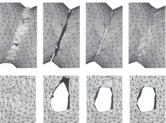
Figure 3: Top row: Merge event. Intersecting triangles are re-moved, holes are joined, followed by mesh improvement. Bottom row: Split event of thin sheet. Triangles whose vertices do not have velocity interpolated from particles are removed, holes are then joined, followed by mesh improvement.
adding a triangle, in the second case we delete the dangling triangle. The remaining holes consist of four or more edges. As a next step we identify pairs of holes that should be joined. To join holes han-dles two types topological events, namely a merge of separate parts of the surface or a split of thin sheets. These are shown in the top and the bottom row of Figure 3, respectively.
To determine whether a pair of holes(ha,hb)should be joined we use two scores, namely
• The number of intersecting triangles pairs(ti,tj)for which at
least one vertex oftiis inhaand at least one vertex oftjis in
hb.
• The number of vertex pairs(vi,vj)withvi∈ha,vj∈hb, and
||vi−vj||2≤gmax.
The total score of a pair of holes is the sum of the two scores divided by the maximum of the number of vertices of the two holes. We usegmax=2lmaxin all examples. To identify close vertices for the second score we use a spatial hash grid containing the hole vertices with grid spacinggmax.
The first score is designed to identify topological merge events in which two parts of the surface collide. The second score is de-signed to capture ruptures of thin sheets. This scoring works well in particle-based liquid simulations with some vertices marked for deletions as will be discussed in Section 3.7.2. In Eulerian simula-tions however, thin sheets do not rupture until the triangles of the two sides intersect due to numerical errors.
Next we sort pairs of holes with a score larger thanβin descending order, where we useβ=1 in all examples. Then we join holes which have not been joined with other holes yet in a greedy fashion. To join a pair of holes(ha,hb), we first identify the closest legal pair of edges(ei,ej)withei∈haandej∈hb. A pair of edges is legal if
a quad formed by the two edges can be triangulated without making the mesh non-manifold, which can be checked by looking upHe. If
there is no such legal pair, we skip joining this pair of holes. After adding the triangulated quad, the two holes now form one big hole.
3.6 Hole Filling
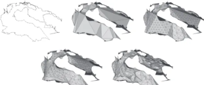
The holes encountered in our examples can have a variety of shapes ranging from being near planar, to complicated and highly curved as shown in Figure 4. At this point, all that is left to do is to fill all holes i.e. triangulate the 3D polygon defined by the border of the hole.
Figure 4: Examples of holes encountered during the simulation. They are not drawn to scale, as the ones on the left are much smaller than the ones in the middle and on the right. The left image shows simple and small holes, the middle image long and thin large holes and the right image large holes with a large area.
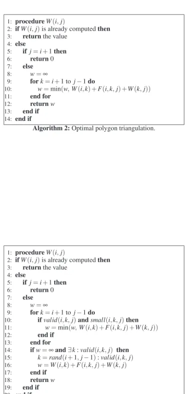
Figure 5: The optimal triangulation of the polygon(i..j)consists of the optimal triangulation of the polygons(i..k)and(k..j)and the triangle(i,k,j), where k is the vertex that minimizes the cost function.
The fastest known algorithm to triangulate a simple polygon has complexityO(n)[Chazelle 1991],[Amato et al. 2000]. However, it tends to produce badly shaped triangles and it is unclear how to generalize the method to triangulate a simple polygon in 3D. On the other hand, finding an optimal triangulation of a 3D sim-ple polygon is a well known application of dynamic programming [Barequet and Sharir 1993]. The optimal triangulation is defined to be the one that minimizes the sum of a cost function over all triangles. Examples of a cost function are the area or the squared edge lengths. However, the time complexity of hole filling based on dynamic programming isO(n3)which is not practical in our appli-cation because holes can sometimes contain more than a thousand vertices.
Therefore we propose an approximate version which runs signifi-cantly faster. Let us first look at the original method. The basic idea to optimally triangulate a polygon with vertices 1. . .nis to define sub-problems, here the problem of finding the optimal triangulation of the polygon from vertexito vertex j. In the optimal triangula-tion of the sub-polygon(i..j)there will be a triangle(i,k,j)and a triangulation of the polygons(i..k)and(k..j)shown in red and blue in Figure 5, respectively.
To compute the costW(i,j)of this optimal triangulation we have to find the optimalk. This can be formulated as the recursive pro-cedure shown in Algorithm 2, whereF(i,k,j)is the cost of the triangle(i,k,j)which we want to minimize. Formulated this way, the valuesW(i,j)are computed multiple times for the sameiand j. The dynamic programming approach reduces this exponential function to a time complexity ofO(n3) by computing each such value exactly once and by storing it in a two dimensional array. Algorithm 3 shows our modification, where
valid(i,k,j) =∀e∈ {(i,k),(k,j),(j,i)}: enot an internal edge ofM0 small(i,k,j) =∀e∈ {(i,k),(k,j),(j,i)}:|e| ≤hmax
F(i,k,j) =|(i,k)|2+|(k,j)|2+|(j,i)|2and hmax=3lmax
1: procedureW(i,j)
2: ifW(i,j)is already computedthen
3: returnthe value
4: else 5: ifj=i+1then 6: return0 7: else 8: w=∞ 9: fork=i+1 toj−1do 10: w=min(w,W(i,k) +F(i,k,j) +W(k,j)) 11: end for 12: returnw 13: end if 14: end if
Algorithm 2:Optimal polygon triangulation.
1: procedureW(i,j)
2: ifW(i,j)is already computedthen
3: returnthe value
4: else 5: ifj=i+1then 6: return0 7: else 8: w=∞ 9: fork=i+1 toj−1do
10: ifvalid(i,k,j)andsmall(i,k,j)then
11: w=min(w,W(i,k) +F(i,k,j) +W(k,j))
12: end if
13: end for
14: ifw=∞and∃k:valid(i,k,j) then
15: k=rand(i+1,j−1):valid(i,k,j) 16: w=W(i,k) +F(i,k,j) +W(k,j) 17: end if 18: returnw 19: end if 20: end if
Figure 6: Our hole filling steps. From top left: hole boundary, minimum sum of squared edge length triangulation, triangles sub-division, triangle relaxations, vertex projection.
The main difference between our method and the original one is that we do not recursive down all possible verticesk. Instead, we cull all non-valid choices and favor small triangles. Our version has several advantages over the original method[Barequet and Sharir 1993].
• If the algorithm succeeds, as indicated byW(1,n)6=∞, the resulting mesh will be manifold, even for highly curved holes. • It not only considers the hole itself but also the surrounding mesh by making sure that internal edges ofM0are not used. • We found a empirical running time in the order ofO(n2)for
large holes.
• We found that if the hole can indeed be triangulated with a manifold triangulation, the algorithm rarely fails.
The reason to favor small triangles with edge lengths in the order oflmaxis that most holes that occur are either small with diameters close tolmaxor long and thin with a thickness close tolmaxas those resulting from merge events or splits of thin sheets (see Figure 3). The optimal triangulation with respect to the sum of squared edge lengths also strongly favors short edges. Therefore, our approxi-mation works well in practice. We also note thatvalid(i,k,j)can be implemented efficiently by looking up the edge hash tableHe
constructed earlier.
Once we have found an approximated optimal triangulation of a hole, we perform a constrained subdivision on the triangulation un-til all internal edges are shorter than lmax and apply the position based relaxations scheme described in Eqn. 3 to the newly gen-erated internal vertices using five iterations andα=0.7. This re-laxation does not shrink the mesh because it is constrained on the boundary. Finally we project the new vertices ontoM if the dis-tance toMis smaller thanlmaxto preserve surface details if possible. Figure 6 shows the complete hole filling process described in this section.
If all holes are filled successfully, we are done. Otherwise, for each hole that cannot be filled by our algorithm, we expand it by deleting all triangles that contain at least one edge of the hole. The listDis then replaced by these deleted triangles. We then go back to ensure that the mesh is manifold and do the hole pairing and hole filling steps again. In our experiments, almost all holes could be filled during the first attempt without expansion. The whole process was never executed more than three times in our examples. We also ran a test on the holes that our algorithm failed to fill and found, by using anO(n3)algorithm, that almost all of them indeed cannot be filled by a manifold triangulation and would require expansion anyway.
3.7 Applications
We have tested our method in a variety of applications with small adaptations.
3.7.1 Surface Tracking with a Grid-based Liquid Solver To track the free surface of a liquid with a grid-based solver, we first use the marching cubes method [Lorensen and Cline 1987b] with a grid spacing oflmax
2 to extract an initial triangulated surface from the initial conditions of the simulation. We also apply one quality improvement step to get a well shaped starting mesh.
At each time step, we first advect the mesh vertices with the fluid velocity field. After this we apply the mesh-based volume conser-vation method of [Thuerey et al. 2010]. Similar to [Wojtan et al. 2010], we extract a signed distance field at the fluid simulation res-olution with grid spacing∆xand use it to enforce the second order free-surface boundary conditions [Enright et al. 2003]. We include the cells overlapped by the surface mesh in the simulation as well. 3.7.2 Surface Tracking with a Particle-Based Liquid Solver For surface tracking with a particle-based liquid solver, we largely follow Yu et al. [2012] but replace Wojtan’s surface tracker [Wojtan et al. 2009] with our own. As in the gird-based simulation case we use the marching cubes mesh with mesh quality improvement as the initial surface.
At each time step we first advect all vertices with the velocity com-puted from nearby simulation particles. For droplets and thin sheets it can happen that no simulation particles are within the kernel ra-dius of certain mesh vertices. To determine the velocities of these vertices we perform velocity interpolation from the vertices whose velocities are known to their one-ring neighbors that do not have velocity information. This can be done without the need of vertex-vertex adjacency information by simply looping through all trian-gles. Vertices without velocity information outside the one-ring are assumed to have a velocity of zero. We also move the vertices without nearby simulation particles by a small amount along the negative normal direction to increase the chance that they will be successfully projected onto the liquid surface.
Next we project all mesh vertices onto the implicit surface defined by the particles using a binary search along the surface normal di-rection. We define the implicit surface to be the iso-contour of the sum of anisotropic kernels as in [Yu and Turk 2010]. During this step, we also mark a vertex for deletion if both of the following conditions apply:
• It fails to get projected onto the surface,
• It is inside the liquid volume or it does not have any nearby simulation particles.
We then apply our method to handle topological changes. Dur-ing the triangle deletion steps, triangles with a marked vertex are deleted as well.
3.7.3 Surface Tracking for Solid Simulation
We demonstrate the use of our method with a particle-based solid simulator based on position-based dynamics [Macklin et al. 2014]. The surface vertices are moved by interpolating the change in po-sition of nearby simulation particles. Those without enough nearby simulation particles get their velocities from neighboring surface vertices. We also mark them for deletion. Similar to particle-based fluid simulations, we delete all triangles with marked ver-tices. However, we also use ray-casting to delete the triangles inside the solid in this case. Our method should be able to track surface of mesh-based solid simulator such as that of Wojtan et al. [2009] as well.
3.7.4 Surface Mesh Modification
We also experiment with surface mesh modifications where the tices are advected based on rules. In this case, after moving the
ver-tices, we run our method to resolve potential topological changes and to improve the mesh quality.
4
Results
We compared the performance of our method with 1. El Topo: [Brochu and Bridson 2009]
2. TopoFixerMC: Topology Fixer using Marching Cubes [Woj-tan et al. 2009] with the subdivision stitching of [Woj[Woj-tan et al. 2010] and
3. TopoFixerCH: Topology Fixer using Convex Hulls [Wojtan et al. 2010]. For this case, we also run an additional mesh im-provement step prior to the topological handling, as suggested in the paper.
For profiling we used the implementations from the authors of the corresponding papers.
We first compared the running times of the above methods using a grid-based solver and a simple scene in which a viscous liquid ball drops into a pool (see Figure 7). The results are shown in Table 1. El Topo, TopoFixerMC, TopoFixerCH and our method took 33, 0.94, 1.14 and 0.67 seconds per time step on average and are about 1, 35, 29 and 49 times faster than El Topo, respectively. For the topology handling step alone, our method is about 1.5 and 1.9 times faster than TopoFixerMC and TopoFixerCH, respectively. As can be seen in the video, TopoFixerMC exhibits some artifacts when thin sheets get deleted toward the end of simulation. El Topo pro-duces high quality results but it is more than an order of magnitude slower than the other methods. We therefore decided to concentrate on TopoFixerMC and TopoFixerCH only in our additional experi-ments.
Next we compared the two TopoFixers and our method in a scene where two water jets collide and form thin sheets simulated with a grid-based solver as shown in Figure 8. In this scene, we keep grow-ing a triangle mesh in the shape of a capsule at the source to repre-sent the volume of water that gets added to the scene. On average, our method is about as fast as TopoFixerMC and 3.3 times faster than TopoFixerCH. On the slowest frame, our method is about as fast as TopoFixerMC and about 14 times faster than TopoFixerCH. As observed in [Wojtan et al. 2010], TopoFixerMC can delete large portions of the liquid when thin sheets merge which results in visual artifacts as the video shows.
We also tried doubling the grid resolution used for TopofixerMC. In this case, the artifacts are reduced but still clearly visible. Now our method is about 1.5 times faster on average and about 4 times faster in the worst case.
In general, TopoFixerCH is able to preserve merging thin sheets better. However, we observed that in some frames it failed to re-solve topological problems. According to the implementation, this happens when the output of QHull [Barber et al. 1996] is not con-sistent with the boundary due to numerical errors or when the out-put mesh is non-manifold. In these cases, the algorithm expands the region of bad cells and retries [Wojtan et al. 2010]. For ev-ery other iteration, TopoFixerCH also jitters the position of certain nodes [Wojtan et al. 2010]. In most instances, the algorithm suc-ceeds after two to three iterations. In some frames of the Jets exam-ple, the method fails after 5 iterations. In such cases, the algorithm reverts to the input mesh. This causes the added capsule mesh at the source to stay at the output which can be seen in the videos. In some rare cases, TopoFixerCH keeps failing without interven-tion. Therefore, we added an extra check. If it fails in two consecu-tive frames, we instead run TopoFixerMC. The output and the run-ning time reported in this paper are based on this variation. We also experimented with doubling the resolution. TopoFixerCH2X suf-fers from the same problem of failing in some consecutive frames
as TopoFixerCH. However, as the grid resolution is increased, when falling back to TopoFixerMC2X, significanlty less volume is lost. Therefore the result is visually quite similar to our method in this case.
Our method is about 4 times faster than TopoFixerCH2X on av-erage and about 11 times faster on the slowest frame. Compared to TopoFixerCH, our method is more robust and runs significantly faster. Our method also retains more liquid volume as can be seen in the bottom row of Figure 8. The running time of our method depends largely on the number of triangles and how many inter-sections are present in the input mesh. On the other hand it is not as sensitive to the numerical values of vertex positions as TopoFix-erCH. This is largely due to the fact that our hole filling algorithm guarantees to produces manifold triangulations which are compati-ble with the hole boundary if feasicompati-ble.
Figure 9 shows an example in which two liquid balls collide in mid air. This scene is simulated with a particle-based liquid solver. Here we compare our method with the on of Yu at al. [Yu et al. 2012] who use TopoFixerMC. The grid size used for TopoFixerMC is the size of bounding box divided by 2lmaxfor the regular case and di-vided bylmaxfor the 2X case. On average, our method takes 0.63s while TopoFixerMC takes 1.04s and TopoFixerMC2X takes 3.40s. The visual quality of our method is roughly the same as the one of TopoFixerMC2X while TopoFixerMC loses a substantial amount of volume due to excessive deletion as the bottom row of Figure 9 shows. Our method is about 1.7 times faster than TopoFixerMC and about 5.4 times faster than TopoFixerMC2X. Our method can directly utilizes information from the particle-based simulation for the inside-outside test. Therefore we neither need to perform ray-casting nor build the 2D spatial hash grid. This reduces the compu-tation time of our method significantly.
We also compared our method with TopoFixerMC and TopoFix-erMC2X in a larger and more open scene. In this case, four jets of liquid are shooting upward to collide and form a fountain as shown in Figure 10. The scene is open and the liquid can flow anywhere. As topology fixer uses a dense grid as the basis for its computation, it is expected to run out of memory for a sufficiently large scene. In-deed, with a 4GB memory limit, TopoFixerMC2X eventually runs out of memory with a grid resolution of 502×328×604. Up until this frame, our method is about 1.5 times faster than TopoFixerMC and about 6 times faster than TopoFixerMC2X on average. As there are a lot of merge events happening at small scale, TopoFixerMC loses a large amount of volume. TopoFixerMC2X loses less vol-ume, but the volume loss is still significant and clearly visible, as Figure 10 and the accompanying video show. We continue the sim-ulation further until liquid touches the ground. At the peak of the size of the liquids’s bounding box TopoFixerMC2X would have re-quired a grid resolution of 2402×265×2736.
Figure 1 shows a projectile hitting a rubber balloon filled with liq-uid. The balloon explodes and the liquid gets ejected outward. The bounding box of the scene expands to occupy a large volume of space. If we were to use TopoFixerMC and TopoFixerMC2X, the grid size required at the peak would be about 2923×2437×2913 and 5848×4875×5828 respectively.
We also tested our method on a particle-based solid simulator. A cow mesh is pushed through bars and undergoes plastic deforma-tion before being torn apart into pieces as can be seen in Figure 11. There are 48k particles in the scene. The simulation including our mesh tracking with out method takes less than a second per frame to compute on average.
Another application of our method is handling topological changes during mesh manipulation as shown in Figure 12. Here the ver-tices of an armadillo mesh are moved along the normals at constant speed. Our method is able to resolve topological changes in this
Figure 7:A liquid ball drop into a pool of water simulated with a grid based solver. This scene is used for comparing our method, El Topo, TopoFixerMC and TopoFixerCH.
Figure 8: Two streams of liquid in collide mid-air to form thin sheets before falling on the floor. This scene is simulated with a grid based fluid solver. Top two rows: Snapshots of the result of our method. Bottom row: A still frame of our method, TopoFixerMC, TopoFixerCH. TopoFixerMC deletes a large amount of volume. application without difficulty as well. We use ray-casting for inside outside test in this case.
4.1 Conclusion and Discussion
We have presented a new fast and robust surface tracking method that is completely grid-free. In Table 4 we compare it qualitatively with recent explicit surface tracking methods. We believe that our approach provides an attractive alternative due to its relatively small computational cost and the high quality results it produces. We can use single precision arithmetic for our computations be-cause our algorithm does not rely on numeric results to ensure man-ifoldness of the output. Our hole filling algorithm ensures mani-foldness only through topological information.
We are currently in the process of implementing our algorithm on the GPU since most of the steps can be done in parallel. Also our method only needs triangle-vertex adjacency information which simplifies a parallel implementation.
While our method handles most scenarios robustly, there are certain stress cases. If the input mesh has a large number of connected in-tersecting triangles that cannot be resolved by the smoothing step, our algorithm creates a large hole that needs to be filled. In this case all the detail from the original mesh is lost. If an entire connected component is involved, our algorithm would delete the entire struc-ture. Fortunately, in practice this only happens for small droplets whose size is smaller thanlmax.
Our method also does not guarantee that the resulting mesh is always totally self-intersection free. However, remaining self-intersections, if they exist, are usually quite small in practice be-cause they stem from numerical errors or from smoothing and from projection onto the old surface. They tend to appear in turbulent areas where a lot of topological changes occur, which makes them difficult to notice visually.
Our method currently chooses the pair of holes to merge in a greedy fashion. When a hole can be matched with more than one other
Figure 9: Two liquid balls colliding in mid-air simulated with a particle-based liquid simulation. Top two rows: Snapshots of our method. Bottom row: Result of Our method, TopoFixerMC and TopoFixerMC2X. TopoFixerMC deletes a significant amount of vol-ume while our method and TopoFixerMC2X are visually similar.
Figure 10:Four streams of liquid being shot up in the air at high speed and collide to form thin sheets and tendrils simulated with a particle-based liquid simulation. Top two rows: Snapshots from our method. Bottom row: Our method, TopoFixerMC, TopoFix-erMC2X. TopoFixerMC deletes a significant amount of volume. The volume loss of TopoFixerMC2X is smaller, but still clearly visible.
Figure 11: A solid cow mesh undergoes plastic deformation and is torn apart. The scene is simulated with a particle-based solid simulator. Our method is used for handling topological changes during the simulation.
TopoRes MoveV Topo Improve Total NumTris avg max avg max avg max avg max avg max Ball Drop El Topo - - - 32778.48 57476.56 - - 36111.48 60558.59 161k 197k Ball Drop TopoFixerMC 120×45×120 48.09 62.50 751.30 1574.22 143.45 207.03 3835.38 4835.94 194k 247k Ball Drop TopoFixerCH 120×45×120 42.29 53.34 960.82 3065.43 139.74 215.58 3695.01 5906.74 193k 242k Ball Drop Our - 42.22 66.77 507.63 712.04 123.32 170.10 3231.86 3692.32 194k 237k Jets TopofixerMC 100×50×100 98.02 166.95 2158.56 3690.43 447.26 785.66 5771.94 9237.40 419k 597k Jets TopofixerMC2X 200×100×200 105.24 197.18 3493.30 14928.22 484.74 887.24 7223.62 20782.48 459k 685k Jets TopofixerCH 100×50×100 105.57 264.34 7668.62 53422.37 466.83 1302.57 11366.39 59327.59 477k 972k Jets TopofixerCH2X 200×100×200 104.65 196.43 10020.49 43744.14 462.74 967.92 13713.25 49246.89 473k 726k Jet Our - 128.26 225.10 2338.34 3797.85 572.44 1782.75 6003.24 9332.62 567k 823k
Table 1: Timing per step for scenes that use 3D Eulerian Liquid Simulation. TopoRes is the grid resolution for TopoFixer, MoveV is the time needed for advecting vertex positions, Topo is the time needed for handling topological changes, Improve is the time for improving mesh quality, Total is the total simulation time and NumTris is the number of triangles of the surface mesh. Note that El Topo combines moving vertices, topological changes and mesh improvement into one step. The timing is in milliseconds. The ball drops and hets are simulated with grid resolutions of120×45×120and100×50×100respectively. The minimum and maximum edge lengths of their surface trackers and mesh quality improvement step are 0.00208-0.00833 and 0.0005-0.005 respectively.
MaxTopoRes Topo Improve Total NumTris
avg max avg max avg max avg max
Ball Splash TopoFixerMC 71×52×71 1043.06 2793.95 316.82 667.15 1557.24 3726.87 157k 216k
Ball Splash TopoFixerMC2X 142×104×142 3401.91 25640.63 444.93 1226.56 4052.21 27128.91 224k 398k
Ball Splash Our - 627.75 2034.18 319.28 950.50 1126.98 3265.93 200k 332k
Fountain* TopoFixerMC 502×328×604 2249.94 7240.47 418.12 850.82 3095.26 9042.72 339k 612k
Fountain* TopoFixerMC2X 125×170×125 8514.42 38207.64 546.38 1340.21 9430.58 41284.01 445k 949k
Fountain* TopoFixerOur - 1466.38 4277.34 560.25 1464.21 2472.64 6721.18 460k 1044k
Fountain TopoFixerMC 737×45×715 8778.20 44859.38 1015.65 2862.68 10112.35 48263.41 828k 2047k
Fountain Our - 6879.84 15605.56 1467.93 3054.90 8771.97 19607.96 1197k 2184k
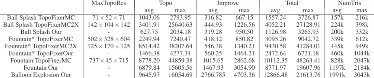
Balloon Explosion Our - 9645.97 16054.69 2766.785 4703.36 12866.48 21613.76 1991k 3043k
Table 2:Timing per step for scenes that use a particle-based simulation. TopoSpacing is the grid spacing used for TopoFixer, MaxTopoRes is the maximum resolution of the grid of TopoFixer encountered during the simulation, Topo is the time needed for handling topological changes, Improve is the time for improving the mesh quality, Total is the total simulation time, NumTris is the number of triangles of the surface mesh. Note that TopoFixerMC2X runs out of memory in the Fountain Scene. Fountain* refers to statistics up to the last frame before TopoFixerMC2X runs out of memory. Fountain is the full sequence run with our method. The Ball splash, Fountain and Balloon scenes use up to 34k, 1311k and 1233k simulation particles, respectively. The minimum and maximum edge lengths of their surface trackers and mesh quality improvement step are 0.005-0.05, 0.0025-0.025,and 0.000078-0.00078 respectively.
Build 3D Hash Find Intersection Remove Topo Noise Build 2D Hash Delete Tris Ensure Manifold Hole Join&Fill NumTris
avg max avg max avg max avg max avg max avg max avg max avg max
BallDrop 102.20 135.63 327.36 489.74 - - 40.03 54.99 31.47 48.16 3.13 8.06 3.48 9.16 194k 237k Jets 430.45 641.48 1556.14 2360.35 - - 134.17 180.47 261.31 561.52 26.19 71.29 26.91 45.90 567k 823k BallsSplash 179.49 327.15 337.01 671.88 89.08 868.17 - - 1.36 2.93 13.50 101.56 11.74 98.63 200k 332k Fountain 1320.98 2611.13 3469.14 7301.65 1558.13 4419.53 - - 11.24 23.81 262.82 1458.39 227.81 1096.49 1197k 2184k Balloon 2345.78 3410.16 6496.80 10636.72 327.12 883.79 - - 24.34 62.50 187.49 576.56 197.90 360.94 1991k 3043k Cow 127.74 250.00 221.82 656.25 - - 62.12 234.39 1.27 31.25 4.94 46.88 9.18 78.13 88k 106k Armadillo 268.52 479.67 646.07 1406.74 - - 66.30 122.84 79.08 133.30 6.76 15.14 8.70 16.11 317k 530k
Figure 12:An armadillo mesh whose vertices move outward along their normal at constant speed. Our method is used to handle the topological changes.
hole, our method may not choose the optimum pair. Fortunately this tends to only happen in chaotic regions where artifacts are less no-ticeable. In certain cases, it might make sense to join multiple holes simultaneously. Our method currently handles this over multiple time steps, which may be undesirable in some cases. Addressing these cases is an interesting area of future work.
Another idea for future work is to extend our method to handle multi-materials as Los Topos [Da et al. 2014] or El Topo[Brochu and Bridson 2009] do. This would require changes in many steps of the algorithm.
Method Speed Quality Unbounded Domain
El Topo [Brochu and Bridson 2009] * ***** Yes
Extended marching cube [M¨uller 2009] ***** * No
TopoFixerMC [Wojtan et al. 2009] **** ** No
TopoFixerCH [Wojtan et al. 2010] ** **** No
Our work **** **** Yes
Table 4:A qualitative comparison between our method and other explicit surface tracking works. Speed refers to the computation time needed. Quality refers to how much surface detail is preserved in the output compared to the input mesh.
Acknowledgements
We would like to thank the anonymous reviewers for their help-ful suggestions and comments. We thank Chris Wojtan and Morten Bojsen-Hansen for providing the TopoFixer and mesh improvement codes. We also thank the members of the NVIDIA PhysX and APEX groups for their valuable inputs and support.
References
ADAMS, B., PAULY, M., KEISER, R.,ANDGUIBAS, L. J. 2007. Adaptively sampled particle fluids. ACM Trans. Graph. 26 (July).
AMATO, N. M., GOODRICH, M. T.,ANDRAMOS, E. A. 2000. Linear-time triangulation of a simple polygon made easier via randomization. InIn Proc. 16th Annu. ACM Sympos. Comput. Geom, 201–212.
ATTENE, M., CAMPEN, M.,ANDKOBBELT, L. 2013. Polygon mesh repairing: An application perspective.ACM Comput. Surv. 45, 2 (Mar.), 15:1–15:33.
ATTENE, M. 2010. A lightweight approach to repairing digitized polygon meshes.The Visual Computer 26, 11, 1393–1406. BARBER, C. B., DOBKIN, D. P., ANDHUHDANPAA, H. 1996.
The quickhull algorithm for convex hulls.ACM Transactions on Mathematical Software 22, 4, 469–483.
BAREQUET, G.,ANDSHARIR, M. 1993. Filling gaps in the bound-ary of a polyhedron. Computer Aided Geometric Design 12, 207–229.
BARGTEIL, A. W., GOKTEKIN, T. G., O’BRIEN, J. F., AND STRAIN, J. A. 2006. A semi-Lagrangian contouring method for fluid simulation.ACM Trans. Graph. 25, 1 (Jan.), 19–38.
BERNSTEIN, G. L., ANDWOJTAN, C. 2013. Putting holes in holey geometry: Topology change for arbitrary surfaces. ACM Trans. Graph. 32, 4 (July), 34:1–34:12.
BLINN, J. F. 1982. A generalization of algebraic surface drawing. ACM Trans. Graph. 1, 3 (July), 235–256.
BORODIN, P., NOVOTNI, M.,ANDKLEIN, R. 2002. Progressive gap closing for meshrepairing. InAdvances in Modelling, Ani-mation and Rendering, J. Vince and R. Earnshaw, Eds. Springer London, 201–213.
BREDNO, J., LEHMANN, T.,ANDSPITZER, K. 2003. A general discrete contour model in two, three, and four dimensions for topology-adaptive multichannel segmentation. Pattern Analysis and Machine Intelligence, IEEE Transactions on 25, 5 (May), 550–563.
BROCHU, T.,ANDBRIDSON, R. 2009. Robust topological oper-ations for dynamic explicit surfaces.SIAM Journal on Scientific Computing 31, 4, 2472–2493.
CAMPEN, M.,ANDKOBBELT, L. 2010. Exact and robust (self-)intersections for polygonal meshes.Comput. Graph. Forum 29, 2, 397–406.
CHAZELLE, B. 1991. Triangulating a simple polygon in linear time.Discrete Comput. Geom. 6, 5 (Aug.), 485–524.
DA, F., BATTY, C., AND GRINSPUN, E. 2014. Multimaterial mesh-based surface tracking. ACM Trans. on Graphics (SIG-GRAPH 2014).
ENRIGHT, D., MARSCHNER, S., ANDFEDKIW, R. 2002. Ani-mation and rendering of complex water surfaces. ACM Trans. Graph. 21, 3 (July), 736–744.
ENRIGHT, D., NGUYEN, D., GIBOU, F.,ANDFEDKIW, R. 2003. Using the particle level set method and a second order accurate pressure boundary condition for free surface flows. InProc. 4th ASME-JSME Joint Fluids Eng. Conf., 2003–45144.
ENRIGHT, D., LOSASSO, F., AND FEDKIW, R. 2005. A fast and accurate semi-Lagrangian particle level set method. Com-put. Struct. 83, 6-7 (Feb.), 479–490.
GUZIEC, A., TAUBIN, G., LAZARUS, F.,ANDHORN, W. 2001. Cutting and stitching: Converting sets of polygons to manifold surfaces.IEEE Trans. Vis. Comput. Graph. 7, 2, 136–151. HU, P., WANG, C., LI, B.,ANDLIU, M. 2012. Filling holes in
triangular meshes in engineering.JSW 7, 1, 141–148.
JUN, Y. 2005. A piecewise hole filling algorithm in reverse engi-neering.Computer-Aided Design 37, 2, 263 – 270.
LIEPA, P. 2003. Filling holes in meshes. InProceedings of the 2003 Eurographics/ACM SIGGRAPH Symposium on Geometry Pro-cessing, Eurographics Association, Aire-la-Ville, Switzerland, Switzerland, SGP ’03, 200–205.
LORENSEN, W. E.,ANDCLINE, H. E. 1987. Marching cubes: A high resolution 3d surface construction algorithm. SIGGRAPH Comput. Graph. 21, 4 (Aug.), 163–169.
LORENSEN, W. E.,ANDCLINE, H. E. 1987. Marching cubes: A high resolution 3D surface construction algorithm. SIGGRAPH Comput. Graph. 21(August), 163–169.
MACKLIN, M., M ¨ULLER, M., CHENTANEZ, N., ANDKIM, T. 2014. Unified particle physics for real-time applications. ACM Trans. Graph. 33, 4, 153.
M ¨OLLER, T. 1997. A fast triangle-triangle intersection test. Jour-nal of Graphics Tools 2, 25–30.
M ¨ULLER, M. 2009. Fast and robust tracking of fluid surfaces. In Proceedings of the 2009 ACM SIGGRAPH/Eurographics Sym-posium on Computer Animation, ACM, New York, NY, USA, SCA ’09, 237–245.
OSHER, S., AND SETHIAN, J. A. 1988. Fronts propagating with curvature-dependent speed: Algorithms based on hamilton-jacobi formulations.Journal of Computational Physics 79, 1, 12 – 49.
PAULCHEW, L. 1989. Constrained delaunay triangulations. Algo-rithmica 4, 1-4, 97–108.
PAVIC, D., CAMPEN, M., AND KOBBELT, L. 2010. Hybrid booleans.Computer Graphics Forum 29, 1, 75–87.
PERNOT, J.-P., MORARU, G.,ANDVRON, P. 2006. Filling holes in meshes using a mechanical model to simulate the curvature variation minimization. Computers & Graphics 30, 6, 892 – 902.
PODOLAK, J.,ANDRUSINKIEWICZ, S. 2005. Atomic volumes for mesh completion. InSymposium on Geometry Processing. PONS, J.-P., AND BOISSONNAT, J.-D. 2007. Delaunay
de-formable models: Topology-adaptive meshes based on the re-stricted delaunay triangulation. InComputer Vision and Pattern Recognition, 2007. CVPR ’07. IEEE Conference on, 1–8. SHEWCHUK, J. R. 1996. Adaptive precision floating-point
arith-metic and fast robust geometric predicates. Discrete & Compu-tational Geometry 18, 305–363.
STANCULESCU, L., CHAINE, R., AND CANI, M.-P. 2011. Freestyle: Sculpting meshes with self-adaptive topology. Com-put. Graph.-UK 35, 3 (June), 614–622. Special Issue: Shape Modeling International (SMI) Conference 2011.
STRAIN, J. 2001. A fast semi-Lagrangian contouring method for moving interfaces. Journal of Computational Physics 170, 1, 373 – 394.
TESCHNER, M., HEIDELBERGER, B., MUELLER, M.,
POMER-ANETS, D.,ANDGROSS, M. 2003. Optimized spatial hashing
for collision detection of deformable objects. 47–54.
THUEREY, N., WOJTAN, C., GROSS, M.,ANDTURK, G. 2010. A Multiscale Approach to Mesh-based Surface Tension Flows. ACM Transactions on Graphics (SIGGRAPH) 29 (4)(July), 10. WOJTAN, C., THUREY, N., GROSS¨ , M.,ANDTURK, G. 2009.
Deforming meshes that split and merge.ACM Trans. Graph. 28, 3 (July), 76:1–76:10.
WOJTAN, C., THUREY, N., GROSS¨ , M.,ANDTURK, G. 2010. Physics-inspired topology changes for thin fluid features. ACM Trans. on Graphics (Proc. SIGGRAPH) 29, 3.
YU, J.,ANDTURK, G. 2010. Reconstructing surfaces of particle-based fluids using anisotropic kernels. In Proceedings of the 2010 ACM SIGGRAPH/Eurographics Symposium on Computer Animation, Eurographics Association, Aire-la-Ville, Switzer-land, SwitzerSwitzer-land, SCA ’10, 217–225.
YU, J., WOJTAN, C., TURK, G.,ANDYAP, C. 2012. Explicit mesh surfaces for particle based fluids.EUROGRAPHICS 2012 30, 41–48.
ZAHARESCU, A., BOYER, E., ANDHORAUD, R. 2007. Trans-forMesh : A Topology-Adaptive Mesh-Based Approach to Sur-face Evolution. InAsian Conference on Computer Vision, 166– 175.
ZHAO, W., GAO, S.,ANDLIN, H. 2007. A robust hole-filling algorithm for triangular mesh. InComputer-Aided Design and Computer Graphics, 2007 10th IEEE International Conference on, 22–22.
ZHU, Y., ANDBRIDSON, R. 2005. Animating sand as a fluid. ACM Trans. Graph. 24, 3 (July), 965–972.