Zhan, Z-H., Zhang, J.,
Li, Y.
and Shi, Y-H.
Orthogonal learning particle
swarm optimization.
IEEE Transactions on Evolutionary Computation
, 99
. p. 1. ISSN 1089-778X
http://eprints.gla.ac.uk/44801/
Deposited on: 16 November 2010
Enlighten – Research publications by members of the University of Glasgow
http://eprints.gla.ac.uk
Orthogonal Learning Particle Swarm Optimization
Zhi-Hui Zhan,
Student Member, IEEE,Jun Zhang,
Senior Member, IEEE,Yun Li,
Member, IEEE,and Yu-Hui Shi,
Senior Member, IEEEAbstract—Particle swarm optimization (PSO) relies on its
learning strategy to guide its search direction. Traditionally, each particle utilizes its historical best experience and its neigh-borhood’s best experience through linear summation. Such a learning strategy is easy to use, but is inefficient when searching in complex problem spaces. Hence, designing learning strategies that can utilize previous search information (experience) more efficiently has become one of the most salient and active PSO research topics. In this paper, we proposes an orthogonal learning (OL) strategy for PSO to discover more useful information that lies in the above two experiences via orthogonal experimental design. We name this PSO as orthogonal learning particle swarm optimization (OLPSO). The OL strategy can guide particles to fly in better directions by constructing a much promising and efficient exemplar. The OL strategy can be applied to PSO with any topological structure. In this paper, it is applied to both glob-al and locglob-al versions of PSO, yielding the G and OLPSO-L algorithms, respectively. This new learning strategy and the new algorithms are tested on a set of 16 benchmark functions, and are compared with other PSO algorithms and some state of the art evolutionary algorithms. The experimental results illustrate the effectiveness and efficiency of the proposed learning strategy and algorithms. The comparisons show that OLPSO significantly improves the performance of PSO, offering faster global conver-gence, higher solution quality, and stronger robustness.
Index Terms—Global optimization, orthogonal experimental
design (OED), orthogonal learning particle swarm optimization (OLPSO), particle swarm optimization (PSO), swarm intelli-gence.
I. Introduction
P
ARTICLE swarm optimization (PSO) algorithm is a global optimization method originally developed by Kennedy and Eberhart [1], [2]. It is a swarm intelligence [3] algorithm that emulates swarm behaviors such as birds flocking and fish schooling. It is a population-based itera-tive learning algorithm that shares some common character-istics with other evolutionary computation (EC) algorithms [4]. However, PSO searches for an optimum through each Manuscript received September 16, 2009; revised January 6, 2010 and February 10, 2010. This work was supported in part by the National Natural Science Foundation of China Joint Fund with Guangdong, under Key Project U0835002, by the National High-Technology Research and Development Program (“863” Program) of China, under Grant 2009AA01Z208, and by the Suzhou Science and Technology Project, under Grant SYJG0919.Z.-H. Zhan and J. Zhang are with the Department of Computer Science, Sun Yat-Sen University, Guangzhou 510275, China, with the Key Laboratory of Digital Life, Ministry of Education, China, and also with the Key Laboratory of Software Technology, Education Department of Guangdong Province, China (e-mail: [email protected]).
Y. Li is with the Department of Electronics and Electrical Engineering, University of Glasgow, Glasgow G12 8LT, U.K.
Y.-H. Shi is with the Research and Postgraduate Office and the Department of Electrical and Electronic Engineering, Xi’an Jiaotong-Liverpool University, Jiangsu 215123, China.
Digital Object Identifier 10.1109/TEVC.2010.2052054
particle flying in the search space and adjusting its flying trajectory according to its personal best experience and its neighborhood’s best experience rather than through particles undergoing genetic operations like selection, crossover, and mutation [5]. Owing to its simple concept and high efficiency, PSO has become a widely adopted optimization technique and has been successfully applied to many real-world problems [6]–[13].
The salient feature of PSO lies in its learning mechanism that distinguishes the algorithm from other EC techniques [5]. When searching for a global optimum in a hyperspace, particles in a PSO fly in the search space according to guiding rules. It is the guiding rules that make the search effective and efficient. In the traditional PSO, the rules are the mechanism that each particle learns from its own best historical experience and its neighborhood’s best historical experience [1]. According to the method of choosing the neighborhood’s best historical experience, PSO algorithms are traditionally classified into global version PSO (GPSO) and local version PSO (LPSO). In GPSO, a particle uses the best historical experience of the entire swarm as its neighborhood’s best historical experience. In LPSO, a particle uses the best historical experience of the particle in its neighborhood which is defined by some topological structure, such as the ring structure, the pyramid structure, or the von Neumann structure [14]–[16]. Without loss of generality, this paper aims at improving the performance of both the GPSO and the LPSO with the ring structure, where a particle takes its left and right particles (by particle index) as its neighbors [2].
In both GPSO and LPSO, the information of a particle’s best experience and its neighborhood’s best experience is utilized in a simple way, where the flying is adjusted by a simple learning summation of the two experiences which will be given in (1) in Section II-A. However, this is not necessarily an efficient way to make the best use of the search information in these two experiences. For example, in one case, it may cause an “os-cillation” phenomenon [17] because the guidance of the two experiences may be in opposite directions. This is inefficient to the search ability of the algorithm and delays the convergence speed. In another case, the particle may suffer from the “two steps forward, one step back” phenomenon [18] that some components of the solution vector may be improved by one exemplar but may be deteriorated by the other. This is because that one exemplar may have good values on some dimensions of the solution vector while the other exemplar may have good values on some other dimensions. Hence, how to discover more useful information embedded in the two exemplars and 1089-778X/$26.00 c2010 IEEE
thus how to utilize the information to construct an efficient and promising exemplar to guide the particle flying steadily toward the global optimal region are important and challenging research issues that PSO researchers need to pay attention to. Because orthogonal experimental design (OED) offers an ability to discover the best combination levels for differ-ent factors with a reasonably small number of experimdiffer-ental samples [19], [20]. In this paper, we propose to use the OED method to construct a promising learning exemplar. Here, OED is used to discover the best combination of a particle’s best historical position and its neighborhood’s best historical position. The orthogonal experimental factors are the dimensions of the problem and the levels of each dimension (factor) are the two choices of a particle’s best position value and its neighborhood’s best position value on this correspond-ing dimension. This way, the best combination of the two exemplars can be constructed to guide the particle to fly more steadily, rather than oscillatory, because only one constructed exemplar is used for the guidance. It is thus expected for a particle to fly more promisingly toward the global optimum because the constructed exemplar makes the best use of the search information of both the particle’s best position and its neighborhood’s best position.
In this paper, the OED is used to form an orthogonal learning (OL) strategy for PSO to discover and preserve useful information of a particle’s best position and its neighborhood’s best position. Owing to the OEDs orthogonal test ability and prediction ability, the OL strategy could construct a guidance exemplar with an ability to predict promising search directions toward the global optimum, therefore results in faster PSO convergence speed and higher solution accuracy. The OL strategy is expected to bring better learning efficiency to PSO and hence better global optimization performance. This learning strategy is applicable to any kind of PSO paradigms, including both GPSO and LPSO. In this paper, the OL strategy-based PSO is termed as orthogonal learning particle swarm optimization (OLPSO). Its advantages will be demonstrated by comparing it with PSOs using traditional learning strategy and with other improved PSOs. Moreover, the OLPSO algorithm is as easy to understand as the traditional PSO and retains the simplicity of PSO.
The rest of the paper is organized as follows. In Section II, the framework of PSO is presented and the researches on improved PSOs are reviewed. In Section III, the OLPSO algorithm is proposed by first discussing the deficiency of tra-ditional learning strategy and then developing the OL strategy. In Section IV, the benchmark functions are used to test OLPSO and to compare it with the PSOs using traditional learning strategy, various improved PSO algorithms, and some state of the art evolutionary algorithms reported in the literatures, in order to verify the effectiveness and efficiency of the OL strategy and the OLPSO in solving global optimization problems. Finally, conclusions are given in Section V.
II. PSO
A. PSO Framework
When searching in aD-dimensional hyperspace, each parti-cleihas a velocity vectorVi= [vi1,vi2, . . . ,viD] and a position
vector Xi = [xi1, xi2, . . . , xiD] to indicate its current state,
whereiis a positive integer indexing the particle in the swarm andDis the dimensions of the problem under study. Moreover, particlei will keep its personal historical best position vector
Pi= [pi1,pi2, . . . ,piD]. The best position of all the particles in
theith particle’s neighborhood (the neighborhood of a particle is defined by a topology structure, e.g., the neighborhood of particle i includes the particles i–1, i, and i+1 in a ring topology structure) is denoted as Pn = [pn1, pn2, . . . , pnD].
The vectorsViandXiare initialized randomly and are updated
by (1) and (2) generation-by-generation through the guidance of Pi andPn
vid=vid+c1r1d(pid−xid) +c2r2d(pnd−xid) (1)
xid =xid +vid. (2)
Coefficientsc1andc2are acceleration parameters which are
commonly set to 2.0 or are adaptively controlled according to the evolutionary states [21]. Ther1d andr2d are two randomly
generated values within range [0, 1] for thedth dimension. In order to control the flying velocity within a reasonable range, a positive valueVMAXd is used to clamp the updated velocity. If |vid|exceedsVMAXd, then it is set tosign(vid)VMAXd. However,
the updated position xid needs not to be clamped if only the
particles within the search space will be evaluated. In this way, all the particles will be drawn back to the range byPiandPn
which are both within the search space [22].
To control or adjust the flying velocity, however, an inertia weight or a constriction factor is introduced by Shi and Eberhart [23], and Clerc and Kennedy [24], [25], respectively. Using inertia weightω, (1) is modified to be (3), whilst using the constriction factor χ, (1) is modified to be (4)
vid =ωvid+c1r1d(pid −xid) +c2r2d(pnd−xid) (3) vid =χ[vid+c1r1d(pid−xid) +c2r2d(pnd−xid)] (4a) where χ= 2 2−ϕ−ϕ2−4ϕ (4b) ϕ=c1+c2. (4c)
In (3), ω usually decreases linearly from 0.9 to 0.4 during the run time [23] whereas χ in (4) is preferably set to be 0.729 together with c1 = c2 = 2.05 [24], [25]. Moreover, the
parameter VMAXd can be omitted in a PSO with constriction
factor. However, as pointed out in [26], the inertia weight and the constriction factor are mathematically equivalent when (4b) and (4c) are met. Without loss of generality, this paper concentrates on the PSO with inertia weight.
B. Improved PSOs
Since its introduction in 1995, PSO has been widely ap-plied to many real-world problems and variants of modified PSOs have been reported in the literature, with enhanced search performance, especially for multimodal optimization
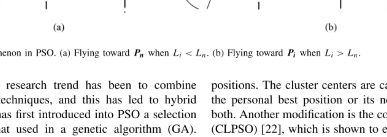
Fig. 1. Oscillation phenomenon in PSO. (a) Flying towardPnwhenLi< Ln. (b) Flying towardPiwhenLi> Ln.
problems. One active research trend has been to combine PSO with other EC techniques, and this has led to hybrid PSOs. Angeline [27] has first introduced into PSO a selection operator similar to that used in a genetic algorithm (GA). Hybridization of PSO with GA has also been applied to recurrent artificial neural network design [28]. Apart from selection [27], crossover [29], and mutation [30] operations that have been adopted from GAs, more other operations have also been utilized. A PSO algorithm with a cooperative approach called CPSO-Sk was proposed in [18], and a
CPSO-Hk algorithm combining the standard PSO with the
CPSO-Sk was shown offering a significant improvement over the
standard PSO [18]. Further, a re-initialization operation and a self-organizing hierarchical technique have been used together with time-varying acceleration coefficients in order to bring diversity into the population [31]. In addition, Parsopoulos and Vrahatis [17] have proposed a hybrid of deflection and stretching techniques to overcome local minima and have also proposed a repulsion technique to prevent particles moving toward the previously found minima. Inspired by natural evolution, some researchers have introduced niche [32], [33] and speciation techniques [34] into PSO for the purposes of avoiding swarm crowding too closely and of locating as many optimal solutions as possible.
Topological structures of PSO have also been studied widely and various topologies have been suggested. Kennedy [14], [15] has shown that a small neighborhood might work better on complex or multimodal problems whilst a larger neighborhood is better for simpler or unimodal problems. Further, dynamically changing neighborhood structures have been proposed by Suganthan [35], Hu and Eberhart [36], and Liang and Suganthan [37] in order to avoid deficiencies of fixed neighborhoods. In addition, Peram et al. [38] have suggested updating the particle velocity by three learning components, two of which are the personal best position and the globally best position, and the other is the particle which has a higher fitness and is nearer to the current particle with a maximal fitness-to-distance ratio. Full information of the entire neighborhood is used to guide the particle in a fully informed particle swarm (FIPS) [39]. That is, all members in the neighborhood can offer their search information fairly or weighted by the distance or fitness of their personal best
positions. The cluster centers are calculated in [40] to replace the personal best position or its neighbor’s best position, or both. Another modification is the comprehensive learning PSO (CLPSO) [22], which is shown to enhance the diversity of the population by encouraging each particle to learn from different particles on different dimensions, in the metaphor that the best particle which has the highest fitness does not always offer a better value in every dimension.
III. OLPSO
In this section, the traditional PSO learning mechanism is first introduced, followed by the motivations of developing the new OL strategy. Then, the OED method and implementation of the OL strategy are presented. Two complete OLPSO algorithms are derived at the end of the section.
A. Traditional PSO Learning Mechanism
In the traditional PSO, each particle updates its flying ve-locity and position according to its personal best position and its neighborhood’s best position. The concept is simple and appealing, but this learning strategy can cause the “oscillation” phenomenon [17] and the “two steps forward, one step back” phenomenon [18].
The “oscillation” phenomenon is likely to be caused by lin-ear summation of the personal influence and the neighborhood influence. For the clearness and easiness of understanding, we first simplify (3) as (5) by removing the inertia weight component and the random values
vid = (pid−xid) + (pnd−xid). (5)
In (5), we consider the following case for a maximization problem where the current particleXiis between its personal
best position Pi and its neighborhood’s best position Pn, as
shown in Fig. 1. At first, the distance betweenPnandXimay
be farther than the one betweenPiandXi, as in Fig. 1(a), then
Xi will move towardPn because of its larger pull. However,
as moving toward Pn, the distance between Pi and Xi will
increase, as shown in Fig. 1(b). In this case, the particle will move towardPiinstead. The oscillation would thus occur and
This oscillation phenomenon causes inefficiency to the search ability of the algorithm and delays convergence.
Another related phenomenon of the traditional learn-ing mechanism is the “two step forward, one step back” phenomenon as described in [18]. For example, given a 3-dimension Sphere functionf(X) =x21+x22+x23, whose global minimum point is [0, 0, 0]. Suppose that the current position is Xi = [2, 5, 2], its personal best position is Pi = [0, 2, 5]
and its neighborhood’s best position is Pn = [5, 0, 1]. The
updated velocity isVi= [1,−8, 2] according to (5), and thus
the new position is Xi = Xi + Vi = [3, −3, 4], resulting in
a new position with a cost value of 34 which is worse than
Xi and Pi. Therefore, the particle does not benefit from the
learning fromPi andPn in this generation. However, vectors
PiandPnindeed possess good information in their structures.
For example, if we can discover good dimensions of the two vectors, we can then combine them to form a new guidance vector ofPo= [0, 0, 1] where the first coordinate 0 comes from
Pi while the second and the third coordinates 0 and 1 come
fromPn (with corresponding dimension). Given the guidance
of Po, the updated velocity becomeVi= Po −Xi= [0, 0, 1] −[2, 5, 2] = [−2,−5,−1]; thus the new position isXi =Xi
+ Vi = [0, 0, 1], resulting in a new and better position with
a cost f(Xi) = 1 that makes the particle fly faster toward the
global optimum [0, 0, 0].
B. Motivations of the OL Strategy
The first motivation of the OL strategy is that the simple cases above have illustrated the importance of designing a guidance vector Po that makes an efficient use of search
information from Pi and Pn. If we exhaustively test all the
combinations of Pi and Pn for the best guidance vector Po,
2D trials are need. This is unrealistic in practice due to the
exponential complexity. With the help of OED [19], [20], however, we can devise a relatively good vector fromPi and
Pn through only a few experimental tests. In this paper, the
OED method is used to test the combinations of Pi and Pn
for a betterPo. The test factors are theDdimensions and the
levels in each factor are 2 for choosing fromPi or Pn.
The second motivation of our work is that recent re-search has shown that incorporating OED in EC algorithms can improve their performance significantly [41]–[50]. The OED method was first introduced into GAs by Zhang and Leung [41] to enhance the crossover operator for multicast routing problems. Leung and Wang [42] proposed another orthogonal GA (OGA/Q) using OED to improve the pop-ulation initialization and to enhance the crossover operator. Hu et al. [43] proposed to use OED on chromosomes to detect surrounding regions for better solutions. Studies in [44] used OED further with a factor analysis that predicts the potentially best combinations. The OED has also been introduced to other optimization algorithms such as simulated annealing [45], [46], ant colony optimization [47], and PSO [48]–[50].
The orthogonal PSO (OPSO) reported in [48] uses an “in-telligent move mechanism” (IMM) operation to generate two temporary positions,H andR, for each particleX, according to the cognitive learning and social learning components,
TABLE I
Factors and Levels of the Chemical Experiment Example
Factors A B C
Levels Temp. °C) Time (Min) Alkali (%)
1L1 80 90 5
2L2 85 120 6
3L3 90 150 7
respectively. Then, OED is performed on H and Rto obtain the best position X∗ for the next move, and then the particle velocity is obtained by calculating the difference between the new position X∗ and the current position X. Such an IMM was also used in [49] to orthogonally combine the cognitive learning and social learning components to form the next position, and the velocity was determined by the difference between the new position and the current position. The OED in [50] was used to help generate the initial population evenly. Different from previous work and to go steps further, in this paper, we use the OED to form an orthogonal learning strategy, which discovers and preserves useful information in the personal best and the neighborhood best positions in order to construct a promising and efficient exemplar. This exemplar is used to guide the particle to fly toward the global optimal region.
The third motivation of developing the OL strategy is that the notion of learning strategy has been very appealing in PSO. A comprehensive learning (CL) strategy has been proposed to extend PSO to CLPSO for improved performance on multimodal functions, but it has been weak in refining solutions, resulting in relatively slow convergence and low-solution accuracy on unimodal functions [22]. Therefore, this paper aims to develop the OL strategy to be able to predict a promising search direction toward the global optimum, for faster convergence and higher solution accuracy. Details of the OED method, the OL strategy, and the OLPSO algorithm will be described in the following sections.
C. OED
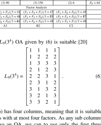
In order to illustrate how to use the OED, a simple example is shown in Table I, which arises from chemical experiments. In this example, the aim is to find the best level combination of the three factors involved to increase the conversion ratio. Table I shows that three factors, which will affect experimental results, are the temperature, time and alkali, denoted as factors A, B, and C, respectively. Moreover, there are three levels (different choices) involved in each factor. For example, the temperature can be 80 °C, 85 °C, or 90 °C. Thus, there are in total 33= 27 combinations of experimental designs. However,
with the help of OED, one can obtain or predict the best combination by testing only few representative experimental cases.
1) Orthogonal Array: The OED method works on a predefined table called an orthogonal array (OA). An OA with N factors and Q levels per factor is always denoted by
LM(QN), whereL denotes the orthogonal array andM is the
TABLE II
Deciding the Best Combination Levels of the Chemical Experimental Factors Using an OED Method
Combinations A: Temperature °C) B: Time (Min) C: Alkali (%) Results
C1 (1) 80 (1) 90 (1) 5 F1= 31 C2 (1) 80 (2) 120 (2) 6 F2= 54 C3 (1) 80 (3) 150 (3) 7 F3= 38 C4 (2) 85 (1) 90 (2) 6 F4= 53 C5 (2) 85 (2) 120 (3) 7 F5= 49 C6 (2) 85 (3) 150 (1) 5 F6= 42 C7 (3) 90 (1) 90 (3) 7 F7= 57 C8 (3) 90 (2) 120 (1) 5 F8= 62 C9 (3) 90 (3) 150 (2) 6 F9= 64 Levels Factor Analysis
L1 (F1+F2+F3)/3 = 41 (F1+F4+F7)/3 = 47 (F1+F6+F8)/3 = 45
L2 (F4+F5+F6)/3 = 48 (F2+F5+F8)/3 =55 (F2+F4+F9)/3 =57
L3 (F7+F8+F9)/3 =61 (F3+F6+F9)/3 = 48 (F3+F5+F7)/3 = 48 OED Results A3 B2 C2
in Table I, theL9(34) OA given by (6) is suitable [20]
L9(34) = ⎡ ⎢ ⎢ ⎢ ⎢ ⎢ ⎢ ⎢ ⎢ ⎢ ⎢ ⎢ ⎢ ⎣ 1 1 1 1 1 2 2 2 1 3 3 3 2 1 2 3 2 2 3 1 2 3 1 2 3 1 3 2 3 2 1 3 3 3 2 1 ⎤ ⎥ ⎥ ⎥ ⎥ ⎥ ⎥ ⎥ ⎥ ⎥ ⎥ ⎥ ⎥ ⎦ . (6)
The OA in (6) has four columns, meaning that it is suitable for the problems with at most four factors. As any sub columns of an OA is also an OA, we can to use only the first three columns (or arbitrary three columns) of the array for the experiment. For example, the first three columns in the first row is [1, 1, 1], meaning that in this experiment, the first factor (temperature), the second factor (time), and the third factor (alkali) are all designed to the first level, that is, 80 °C, 90 minutes, and 5% as given in Table I. Similarly, combination of [1, 2, 2] is used in the second experiment, and so on. The total of nine experiments specified by theL9(34) are presented
in Table II.
2) Factor Analysis: The ability of discovering the best combination of levels is through thefactor analysis(FA). The FA is based on the experimental results of all theM cases of the OA. The FA results are shown in Table II and the process is described as follows.
Letfm denote the experimental result of themth (1≤m≤
M) combination andSnqdenote the effect of theqth (1≤q≤
Q) level in the nth (1 ≤ n ≤ N) factor. The calculation of
Snq is to add up all thefm in which the level isq in the nth
factor, and then divide the total count ofzmnq, as shown in (7)
wherezmnq is 1 if the mth experimental test is with the qth
level of thenth factor, otherwise,zmnq is 0
Snq= M m=1fm×zmnq M m=1zmnq . (7)
In this way, the effect of each level on each factor can be calculated and compared, as shown in Table II. For example, when we calculate the effect of level 1 on factor A, denoted by element A1, the experimental results of C1, C2, and C3
are summed up for (7) because only these combinations are involved in level 1 of factor A. Then, the sum divides the combination number (3 in this case) to yieldSnq (SA1 in this
case). With all theSnq calculated, the best combination of the
levels can be determined by selecting the level of each factor that provides the highest-quality Snq. For a maximization
problem, the larger the Snq is, the better the qth level on
factor n will be. Otherwise, vice versa. As in the maximiza-tion example shown in Table II, the best result is the combi-nation of A3, B2, and C2. Although the combicombi-nation of (A3, B2, C2) itself does not exist in the nine combinations tested, it is discovered by the FA process.
D. OL Strategy
Using the OED method, the original PSO can be modified as an OLPSO with an OL strategy that combines information of
PiandPnto form a better guidance vectorPo. The particle’s
flying velocity is thus changed as
vid =ωvid+crd(pod−xid) (8)
whereωis the same as in (3) andcis fixed to be 2.0, the same as c1 and c2, and rd is a random value uniformly generated
within the interval [0, 1].
The guidance vector Po is constructed for each particle i,
respectively, fromPi andPn as
Po = Pi⊕Pn (9)
where the symbol⊕stands for the OED operation. Therefore, the value pod comes from pid or pnd as the construct result
of OED. With this efficient learning exemplar Po, particle i
adjusts its flying velocity, position and updates its personal best position in every generation. In order to avoid the guidance changing the direction frequently, the vectorPowill be used as
the exemplar for a certain number of generations until it cannot lead the particle to a better position any more. For example, if the personal best positionPi has not been improved for G
generations, then particleiwill reconstruct a newPo by using
Pi andPn. On the other hand, as Po is used for some time
until it cannot improve the position, one problem should be addressed is how to use the information that comes from Pi
and Pn immediately after Pi and Pn go to a better position
during the search process. In our implementations, vector Po
stores only the index of Pi and Pn, not the copy of the
real position values. That is, pod only indicates that the dth
dimension is guided byPiorPn, it does not store the current
value ofpid orpnd. Thus, in the OLPSO algorithm, whenPi
orPn moves to a better position, the new information will be
used immediately by the particle throughPo.
The construction process ofPois described as the following
six steps.
Step 1) An OA is generated as LM(2D) where M =
2log2(D+1), using the procedure as given in
Ap-pendix.
Step 2) Make up M tested solutions Xj (1 ≤ j ≤ M)
by selecting the corresponding value from Pi or Pn
OA is 1, then the corresponding factor (dimension) selectsPi; otherwise, selectsPn.
Step 3) Evaluate each tested solution Xj (1≤ j ≤M), and
record the best (with best fitness) solutionXb.
Step 4) Calculate the effect of each level on each factor and determine the best level for each factor using (7). Step 5) Derive a predictive solutionXpwith the levels
deter-mined in Step 4 and evaluateXp.
Step 6) Comparef(Xb) andf(Xp) and the level combination
of the better solution is used to construct the vector
Po.
In the above process, each of theDdimensions is regarded as a factor and therefore there are D factors in the OED. This results in M = 2log2(D+1) orthogonal combinations
because the level of each factor is two [20]. Therefore the
M is no larger than 2D, which is significantly smaller than the total number of combinations 2D. A method to further
reduce the number of the orthogonal combinations is to divide the dimensions into several disjoint groups and regard each group as a factor. This method also may be good for the problems whose dimensions are not independent of each other. Unfortunately, how many groups should be divided and how to assign different dimensions to different groups are usually problem-dependent and difficult to decide [44]. Therefore, since the problem characteristic is usually unknown, it may be a good choice to regard each dimension as a factor. In fact, by using OED, some factors can be regarded as in the same group when they are with the same level. Therefore, it is without loss of generality to regard each dimension as a factor.
E. OLPSO
The OL strategy is a generic operator and can be applied to any kind of topology structure. If the OL is used for the GPSO, then Pn is Pg. If it is used for the LPSO, then Pn is
Pl. Either for a global or a local version, when constructing
the vector of Po, if Pi is the same as Pn (e.g., for the
globally best particle, Pi and Pg are identical vectors), the
OED makes no contribution. In such a case, OLPSO will randomly select another particle Pr, and then construct Po
by using the information ofPiandPr through the OED.
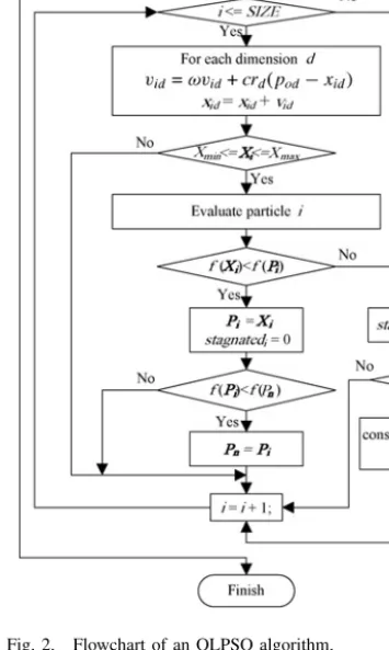
The flowchart of OLPSO is shown in Fig. 2. As discussed in the previous section, the particle will use vectorPo as the
learning exemplar steadily and reconstruct thePoonly after a
stagnation ofPiforGgenerations. As can be imagined, ifGis
too small, the particles will reconstruct the guidance exemplar
Po frequently. This may waste computations on OED when it
is not indeed necessary. Also, the search direction will not be steady ifPochanges frequently. On the other hand, ifGis too
large, the particles will waste much computation on the local optima with aPo which is not effective any longer.
In order to investigate the influence ofGon the performance of the OLPSO algorithm, empirical studies are carried out on relevant functions, namely the Sphere, Rosenbrock, Schwefel, Rastrigrin, Ackley, and Grienwank functions listed in Table III as thef1,f3,f5,f6,f7, andf8, respectively. Different values
for Gfrom 0 to 10 are tested, and two OLPSO versions that based on a global topology (OLPSO-G) and a local topology
Fig. 2. Flowchart of an OLPSO algorithm.
(OLPSO-L) are simulated. The results of the investigation are shown in Fig. 3(a) and (b) with averagely 25 independent runs for the OLPSO-G and the OLPSO-L, respectively. The figures reveal that a value of G around 5 offers the best performance. This also indicates OLPSO indeed benefits from the OL strategy by the steadily guidance of a promising learning exemplar. Therefore, a reconstruction gap of G = 5 is used in this paper.
IV. Experimental Verification and Comparisons
A. Functions Tested and PSOs Compared
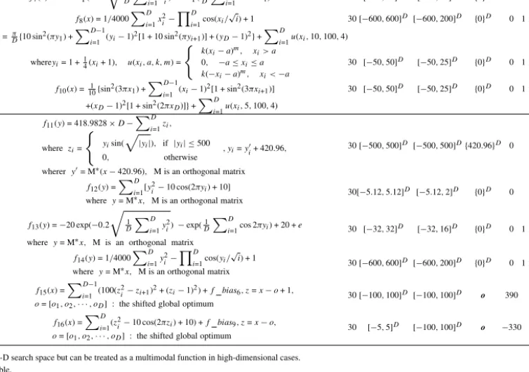
Sixteen benchmark functions listed in Table III are used in the experimental tests. These benchmark functions are widely adopted in benchmarking global optimization algorithms [22], [51], [56]. In this paper, the functions are divided into three groups. The first group includes four unimodal functions, where f1 and f2 are simple unimodal, f3 (Rosenbrock) is
unimodal in a 2-D or 3-D search space but can be treated as a multimodal function in high-dimensional cases [52]–[54], and
f4 is with noisy perturbation. The second group includes six
TABLE III
Sixteen Test Functions Used in the Comparison
Test Function D Search Initialization Global fmin Accept Name Range Range Opt.x∗
Unimodal f1(x) = D i=1x 2 i 30 [−100,100]D [−100,50]D {0}D 0 1×10⁻⁶Sphere [51] f2(x) = D i=1|xi|+ D i=1|xi| 30 [−10,10] D [−10,5]D {0}D 0 1×10⁻⁶Schwefel’sP2.22[51] f3∗(x) = D−1 i=1 [100(xi+1−x 2 i) 2+ (x i−1)2] 30 [−10,10]D [−10,10]D {1}D 0 100 Rosenbrock [51]† f4(x) = D i=1ix 4 i+random[0,1) 30[−1.28,1.28] D[−1.28,0.64]D {0}D 0 0.01 Noise [51] Multimodal f5(x) = 418.9829×D− D i=1xisin( |xi|) 30 [−500,500]D [−500,500]D{420.96}D 0 2000 Schwefel [51] f6(x) = D i=1[x 2 i−10 cos(2πxi) + 10] 30[−5.12,5.12]D [−5.12,2]D {0}D 0 100 Rastrigin [51] f7(x) =−20 exp(−0.2 1 D D i=1x 2 i)−exp(D1 D i=1cos 2πxi) + 20 +e 30 [−32,32] D [−32,16]D {0}D 0 1×10⁻⁶Ackley [51] f8(x) = 1/4000 D i=1x 2 i− D i=1cos(xi/ √ i) + 1 30 [−600,600]D [−600,200]D {0}D 0 1×10⁻⁶Griewank [51]† f9(x) =πD{10 sin2(πy1) + D−1 i=1 (yi−1) 2[1 + 10 sin2(πy i+1)] + (yD−1)2}+ D i=1u(xi,10,100,4) whereyi= 1 +14(xi+ 1), u(xi, a, k, m) = k(xi−a)m, x i> a 0, −a≤xi≤a k(−xi−a)m, x i<−a 30 [−50,50]D [−50,25]D {0}D 0 1×10⁻⁶Generalized Penalized [51] f10(x) =101{sin2(3πx1) + D−1 i=1 (xi−1) 2[1 + sin2(3πx i+1)] 30 [−50,50]D [−50,25]D {0}D 0 1×10⁻⁶ +(xD−1)2[1 + sin2(2πxD)]}+ D i=1u(xi,5,100,4) Rotated and Shifted
f11(y) = 418.9828×D− D i=1zi, wherezi= yisin( |yi|), if |yi| ≤500 0, otherwise , yi=yi+ 420.96,
wherery= M∗(x−420.96), M is an orthogonal matrix
30 [−500,500]D [−500,500]D{420.96}D 0 5000 Rotated Schwefel [22]† f12(y) = D i=1[y 2 i−10 cos(2πyi) + 10]
wherey= M∗x, M is an orthogonal matrix 30[−5.12,5.12]
D [−5.12,2]D {0}D 0 100 Rotated Rastrigin [22]† f13(y) =−20 exp(−0.2 1 D D i=1y 2 i)−exp( 1 D D i=1cos 2πyi) + 20 +e wherey= M∗x, M is an orthogonal matrix
30 [−32,32]D [−32,16]D {0}D 0 1×10⁻⁶Rotated Ackley [22]† f14(y) = 1/4000 D i=1y 2 i− D i=1cos(yi/ √ i) + 1 wherey= M∗x, M is an orthogonal matrix
30 [−600,600]D [−600,200]D {0}D 0 1×10⁻⁶Rotated Griewank [22]† f15(x) = D−1 i=1 (100(z 2 i−zi+1)2+ (zi−1)2) +f bias6, z=x−o+ 1,
o= [o1, o2,· · ·, oD] : the shifted global optimum
30 [−100,100]D [−100,100]D o 390 490 Shifted Rosenbrock [56]† f16(x) = D i=1(z 2 i−10 cos(2πzi) + 10) +f bias9, z=x−o,
o= [o1, o2,· · ·, oD] : the shifted global optimum
30 [−5,5]D [−100,100]D o −330 −230 Shifted
Rastrigin [56]
f3∗is unimodal in a 2-D or 3-D search space but can be treated as a multimodal function in high-dimensional cases. †The function is non-separable.
TABLE IV
PSO Algorithms for Comparison
Algorithm Parameters Settings Reference GPSO ω: 0.9∼0.4,c1=c2= 2.0,VMAXd= 0.2×Range [23]
LPSO ω: 0.9∼0.4,c1=c2= 2.0,VMAXd= 0.2×Range [15]
SPSO ω= 0.721,c1=c2= 1.193,K= 3, withoutVMAX [55] FIPS χ= 0.729, ci= 4.1,VMAXd= 0.5×Range [39] HPSO-TVACω: 0.9∼0.4,c1: 2.5∼0.5,c2: 0.5∼2.5,VMAXd= 0.5×Range [31]
DMS-PSO ω: 0.9∼0.2,c1=c2= 2.0,m= 3,R= 5,VMAXd= 0.2×Range [37]
CLPSO ω: 0.9∼0.4,c= 1.49445,m= 7,VMAXd= 0.2×Range [22]
OPSO ω: 0.9∼0.4,c1=c2= 2.0,VMAXd= 0.5×Range [48]
OLPSO ω: 0.9∼0.4,c= 2.0,G= 5,VMAXd= 0.2×Range − last group includes four rotated multimodal functions and 2 shifted functions defined in [56].
Table III gives the global optimal solution (column 5) and the global optimal value fmin (column 6). Moreover, biased
initializations (column 4) are used according to the definitions in [22] for the functions whose global solution point is at the center of the search range. “Accept” (column 7) is also defined for each test function. If a solution found by an algorithm falls between the acceptable value and the actual global optimum
fmin (column 5), the run is judged to be successful.
Variant PSO algorithms, as detailed in Table IV, are used for comparisons. The parameter configurations are all based on the suggestions in the corresponding references. The first two are traditional PSOs of GPSO [23] and LPSO [15]. The third is the Standard PSO (SPSO) [55]. SPSO is the current standard which is improved by using a random topology, refer to http://www.particleswarm.info/ Programs.html#Standard−PSO−2007 for more details. The fourth is a “fully informed” PSO (FIPS) [39] that uses all the neighbors to influence the flying velocity. The fifth is a “performance-improvement” PSO by improving the accelera-tion coefficients, namely hierarchical PSO with time-varying acceleration coefficients (HPSO-TVAC) [31]. The sixth is a dynamic multi-swarm PSO (DMS-PSO) [37] which is de-signed to improve the topological structure in a dynamic way. The seventh, CLPSO [22], aims to offer a better performance for multimodal functions by using a CL strategy. The eighth, the OPSO [48] algorithm, aims to improve the algorithm by using an OED to generate a better position, not by constructing a learning exemplar as proposed in this paper. These PSO vari-ants are used for comparisons because they are typical PSOs that are reported to perform well on their studied problems. Moreover, they span a wide time interval from 1998 to 2008, which witness the developments of PSO on variant aspects. For OLPSO developed in this paper, we implement the OL strategy in both the global and the local version PSO, resulting in two OLPSO algorithms, the OLPSO-G and the OLPSO-L, respectively. Both will be compared with GPSO, LPSO, SPSO, FIPS, HPSO-TVAC, DMS-PSO, CLPSO, and OPSO.
For a fair comparison among all the PSOs, they are tested using the same population size of 40. As the SPSO in [55] automatically computes a size of 20 for 30-D functions, we both use SPSO with 20 and 40 particles in the experiments. The two SPSO variants are denoted as 20 and SPSO-40, respectively. Furthermore, all the algorithms use the same maximum number of function evaluations (FEs) 2×10⁵ in
each run for each test function. Note that the number of FEs consumed during the construction of the guidance exemplarPo
in OLPSO are included in this maximum FEs number allowed. Also notice that an L32(231) OA [20], [44] is suitable for all
the test functions because they are all 30 dimensional. For the purpose of reducing statistical errors, each algorithm is tested 25 times independently for every function and the mean results are used in the comparison.
B. Solution Accuracy with OL Strategy
The solutions obtained by OLPSOs are compared with the ones obtained by PSOs without OL strategy in Table V. Table V compares the mean values and the standard deviations of the solutions found. The best results are marked in boldface. Thet-test results between G and GPSO, and OLPSO-L and OLPSO-LPSO are also given, respectively.
1) Unimodal Functions: For the four unimodal func-tions, the results show that OLPSOs generally outperform the traditional PSOs. For example, OLPSO-G does better than GPSO on functions f1, f2, and f3 whilst OLPSO-L
outperforms LPSO on functions f1, f2, f3, and f4. The
experimental results show that the OL strategy brings solution with much higher accuracy to the problem. For the very simple unimodal functions f1 and f2, OLPSO-G provides solutions
with the highest quality. However, as the problem becomes more complex, even become multimodal in high dimension, such as the Rosenbrock’s function (f3), the performance of
OLPSO-L is much better. This is in coincidence with the general observation that a LPSO does better than a GPSO on complex problems. This is because a LPSO draws experience from locally best particles, as opposed to the interim global best, and hence avoids a premature convergence, although it could converge more slowly. As for the Noise function (f4), we can observe that OLPSO-G does not show an advantage. This is perhaps because the effect of the OL strategy is largely canceled out by the random fluctuation.
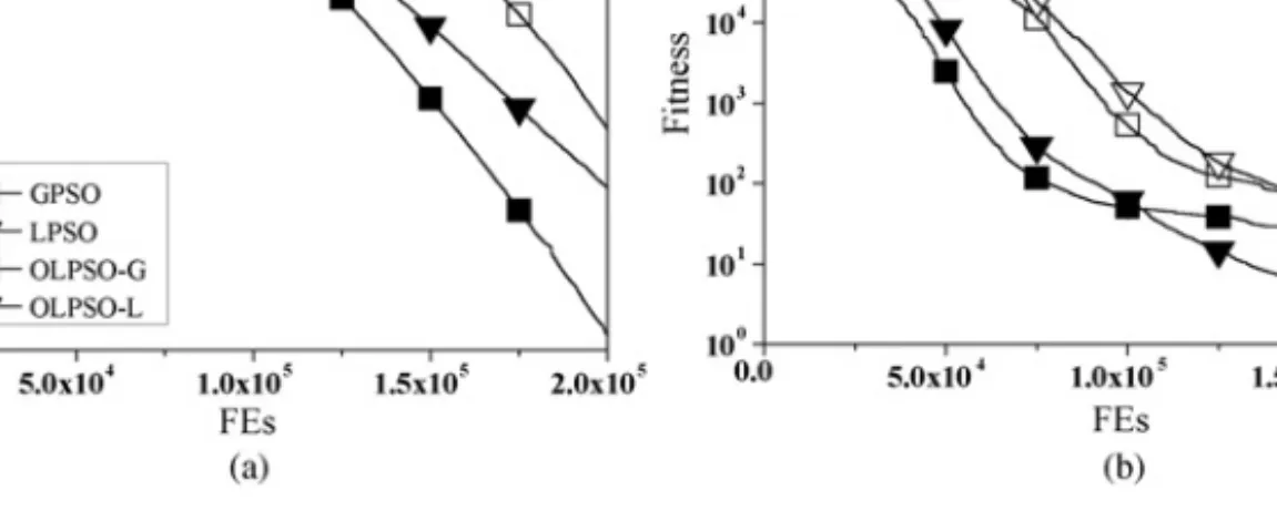
The plots in Fig. 4 show the convergence progress of the mean solution values of the 25 trials during the run for func-tionsf1andf3. It is apparent that OLPSOs perform better than
the traditional PSOs in terms of final solution and convergence speed. It can be observed from the figures that OLPSOs with the OL strategy converge considerably faster than the traditional PSOs (GPSO and LPSO) without an OL strategy.
2) Multimodal Functions: As the efficiency of the OL strategy provides PSO an ability to discover, preserve, and utilize useful information of the learning exemplars, it is expected that OLPSO can avoid local optima and bring about improved performance on multimodal functions. Indeed, the experimental results for functions f5–f10 given in Table V
support this intuition. OLPSO-G surpasses GPSO on all the six multimodal functions. OLPSO-L yields the best perfor-mance among the four PSOs on all the six multimodal functions, in terms of mean solutions and standard deviations. In comparison, GPSO can only reach the global optimum on function f7 and f9 while LPSO on functions f7, f9,
and f10. Best of all, OLPSO-L is able to find the global
optimum on all the functions and only OLPSO-L can show significantly improved performance in reaching the global
TABLE V
Solutions Accuracy (Mean and Standard Deviation) Comparisons Between PSOs With and Without the OL Strategy
Func GPSO OLPSO-G t-Test LPSO OLPSO-L t-Test
f1 2.05×10⁻³²±3.56×10⁻³² 4.12×10−54±6.34×10−54 2.88† 3.34×10⁻¹⁴±5.39×10⁻¹⁴ 1.11×10−38±1.28×10−38 3.10‡ f2 1.49×10⁻²¹±3.60×10⁻²¹ 9.85×10⁻³⁰±1.01×10⁻²⁹ 2.07† 1.70×10⁻¹⁰±1.39×10⁻¹⁰ 7.67×10⁻²²±5.63×10⁻²² 6.12‡ f3 40.70±32.19 21.52±29.92 2.18† 28.08±21.79 1.26±1.40 6.14‡ f4 9.32×10⁻³±2.39×10⁻³ 1.16×10⁻²±4.10×10⁻³ −2.38† 2.28×10⁻²±5.60×10⁻³ 1.64×10⁻²±3.25×10⁻³ 4.96‡ f5 2.48×10³±2.97×10² 3.84×10²±2.17×10² 28.53† 3.16×10³±4.06×10² 3.82×10⁻⁴±0 38.95‡ f6 26.03±7.27 1.07±0.99 17.00† 35.07±6.89 0±0 25.46‡ f7 1.31×10⁻¹⁴±2.08×10⁻¹⁵ 7.98×10⁻¹⁵±2.03×10⁻¹⁵ 8.80† 8.20×10−08±6.73×10−08 4.14×10⁻¹⁵±0 6.09‡ f8 2.12×10⁻²±2.18×10⁻² 4.83×10⁻³±8.63×10⁻³ 3.50† 1.53×10⁻³±4.32×10⁻³ 0±0 1.77 f9 2.23×10⁻³¹±7.07×10⁻³¹ 1.59×10⁻³²±1.03×10⁻³³ 1.46 8.10×10⁻¹⁶±1.07×10⁻¹⁵ 1.57×10⁻³²±2.79×10−48 3.80‡ f10 1.32×10⁻³±3.64×10⁻³ 4.39×10⁻⁴±2.20×10⁻³ 1.03 3.26×10⁻¹³±3.70×10⁻¹³ 1.35×10⁻³²±5.59×10−48 4.41‡ f11 4.61×10³±6.21×10² 4.00×10³±6.08×10² 3.51† 4.50×10³±3.97×10² 3.13×10³±1.24×10³ 5.28‡ f12 60.02±15.98 46.09±12.88 3.39† 53.36±13.99 53.35±13.35 0.00 f13 1.93±0.96 7.69×10⁻¹⁵±1.78×10⁻¹⁵ 10.01† 1.55±0.45 4.28×10⁻¹⁵±7.11×10⁻¹⁶ 17.44‡ f14 1.80×10⁻²±2.41×10⁻² 1.68×10⁻³±4.13×10⁻³ 3.33† 1.68×10⁻³±3.47×10⁻³ 4.19×10⁻⁸±2.06×10⁻⁷ 2.42‡ f15 427.93±54.98 424.75±34.80 0.24 432.33±43.41 415.95±23.96 1.65 f16 −223.18±38.58 −328.57±1.04 13.65† −234.95±18.82 −330±1.64×10⁻¹⁴ 25.36‡
†The value oftwith 48 degrees of freedom is significant atα= 0.05 by a two-tailed test between GPSO and OLPSO-G. ‡The value oftwith 48 degrees of freedom is significant atα= 0.05 by a two-tailed test between LPSO and OLPSO-L.
Fig. 4. Convergence progresses of the PSOs with and without the OL strategy on unimodal functions (a)f1(Sphere) and (b)f3 (Rosenbrock).
optimum 0 on the Rastrigin’s function (f6) and the Griewank’s
function (f8). These experimental results verify that the
OLP-SOs with the OL strategy offer the ability of avoiding local optima to obtain the global optimum robustly in multimodal functions.
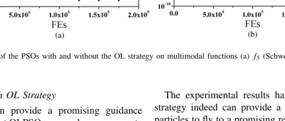
The evolutionary progresses of the PSOs in optimizing the multimodal functionsf5andf6are plotted in Fig. 5. It can be observed that OLPSOs are able to improve solutions steadily for a long period without being trapped in local optima. OLPSO-L appears to exhibit the strongest search ability and can converge to the global optimum 0 in about 1.5×10⁵ FEs
on the Rastrigin’s function. The convergent curves on the Schewefel’s function (f5) also show that OLPSO-L has strong
global search ability to avoid local optima.
3) Rotated and Shifted Functions: Functions f11 to f14
are multimodal functions with coordinate rotation while f15
and f16 are shifted functions. In order to avoid biases of
specific rotations in the tests, a new rotation is computed before each run of the 25 independent trials. Experimental
results for the four rotated multimodal functions are also given in Table V and the evolutionary progresses of f13
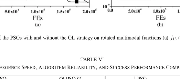
and f14 are plotted in Fig. 6. It appears that all the PSO
algorithms are affected by the coordinate rotation. However, it is interesting to observe that the OLPSO algorithms can still reach the global optima of the rotated Ackley’s function (f13)
and the rotated Grienwank’s function (f14). All the PSOs are trapped by the rotated Schwefel’s function (f11) and the rotated Rastrigin’s function (f12) as they become much more difficult
after coordinate rotation [22]. However, OLPSOs still perform better than traditional PSOs on these two problems. The experimental results also show that OLPSO-G and OLPSO-L outperform GPSO and LPSO, respectively, on the two shifted functionf15andf16. Moreover, only OLPSO-L can obtain the
global optimum−330 on the shifted Rastrigin’s function (f16).
Overall, even though affected by the rotation and the shift, the comparisons still indicate that the OL strategy is beneficial to the PSO performance, and OLPSOs generally perform better than traditional PSOs.
Fig. 5. Convergence progresses of the PSOs with and without the OL strategy on multimodal functions (a)f5 (Schwefel) and (b)f6 (Rastrigin).
C. Convergence Speed with OL Strategy
As the OL strategy can provide a promising guidance exemplarPo, it is natural that OLPSO can reach more accurate
solution with a faster convergence speed. In order to verify this, more experimental results are given and compared in Table VI. The results given there are the average FEs needed to reach the threshold expressed as acceptable solutions specified in Table III. In addition, successful rate (SR%) of the 25 independent runs for each function are also compared. Note that the average FEs are calculated only for the runs that have been “successful.” As some algorithms may not succeed in reaching the acceptable solution every run on some problems, the metric success performance (SP), defined as SP = (Average FEs)/(SR%) [56], is also compared in Table VI.
It can be observed from the table that OLPSO-G and OLPSO-L are constantly faster than GPSO and LPSO, respec-tively, on the tested functions. This indeed shows the advan-tage of the OL strategy in constructing promising exemplar to guide the flying direction for faster optimization speed. Moreover, with a reasonable agreement to the fact that GPSO is always faster than LPSO, OLPSO-G is observed to be faster than OLPSO-L and is also the fastest algorithm among the four contenders. Even the slower OLPSO-L (when compared with OLPSO-G), still converges faster than GPSO (global version but without OL strategy) on most of the functions. For example, in solving the Sphere function (f1), average
numbers of FEs 134 561 and 161 985 are needed by GPSO and LPSO, respectively, to reach the acceptable accuracy 1×10⁻⁶. However, OLPSO-G uses only 89 247 FEs, which indicates that it is the fastest algorithm. OLPSO-L uses 98 337 FEs to obtain the solution, which is faster not only than LPSO, but also than GPSO.
The successful rates shown in the Table VI also indicate that the OL strategy is very promising in bringing a high reliability to PSO. The OLPSOs result in higher algorithm reliability with 100% successful rate on most of the test functions while traditional PSOs are sometimes trapped in the multimodal, rotated, or the shifted problems. Overall, OLPSO-L yields the highest successful rate 93.50% averaged on all the 16 functions, and followed by OLPSO-G, LPSO, and GPSO.
The experimental results have demonstrated that the OL strategy indeed can provide a much better guidance for the particles to fly to a promising region faster. The OLPSOs with the OL strategy are more robust and reliable in solving global optimization problems.
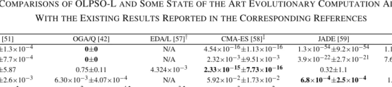
D. Comparisons with Other PSOs
In this section, the OLPSOs will be compared with some other improved PSO variants, namely, SPSO-20, SPSO-40, FIPS, HPSO-TVAC, DMS-PSO, CLPSO, and OPSO, which have been detailed in Section IV-A. The mean and the standard deviation (SD) of the final solutions are given and compared in Table VII. It can be observed that OLPSOs achieve the best solution on most of the functions. SPSO seems to be good at simple unimodal functions and SPSO-20 performs best onf1,
and f2. Also SPSO-20 does best on the Noise function (f4),
and the shifted Rosenbrock function (f15). FIPS performs best
on the rotated Griewank’s function (f14). DMS-PSO yields the
best solution on the rotated Rastrigin’s function (f12). CLPSO
obtains the same best mean solution as OLPSO-L does on the Schewefel’s function (f5) and the shifted Rastrigin function
(f16). Overall, OLPSO-L performs best onf3,f5,f6,f7,f8, f9,f10,f11,f13, andf16, i.e., 10 out of the 16 functions.
On the unimodal functions, OLPSO-G is shown to offer superior performance among all the PSOs except SPSO. Note that the OLPSOs may not be most efficient in solving the problems with random noise, such as f4. Similarly, OPSO
which also uses an OED method (different from the OL strategy proposed in this paper) also encounters difficulties in dealing with this noisy function. This deficiency may be caused by the OED itself being fluctuated by the random noise. On the multimodal functions, OLPSOs generally outperform all the other PSO variants. Only can OLPSO-L and CLPSO obtain high-quality mean solutions with the error value of 10−4 to the Schwefel’s function (f5) and the Rastrigin’s function
(f6), and only OLPSO-L, CLPSO, and FIPS can obtain
high-quality mean solutions with the error value of 10−9 to the
Griewank’s function (f8).
On the coordinate rotated and shifted functions, OLPSOs also generally do better than other PSOs. OLPSO-G can still
Fig. 6. Convergence progresses of the PSOs with and without the OL strategy on rotated multimodal functions (a)f13(Rotated Ackley) and (b)f14(Rotated
Griewank).
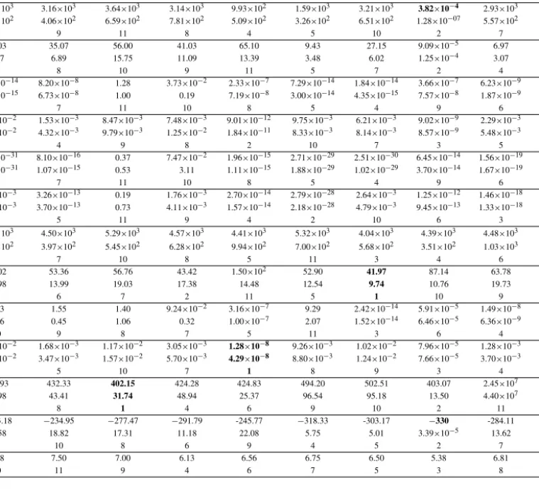
TABLE VI
Convergence Speed, Algorithm Reliability, and Success Performance Comparisons
Function GPSO OLPSO-G LPSO OLPSO-L
FEs SR% SP FEs SR% SP FEs SR% SP FEs SR% SP
f1 134 561 100 134 561 89 247 100 89 247 161 985 100 161 985 98 337 100 98 337 f2 141 262 100 141 262 101 698 100 101 698 171 962 100 171 962 114 441 100 114 441 f3 126 343 100 126 343 78 749 100 78 749 137 934 100 137 934 92 233 100 92 233 f4 171 048 60 285 080 150 238 40 375 595 × 0 × 186 351 4 4 658 775 f5 117 710 8 1 471 375 40 533 100 40 533 × 0 × 51 498 100 51 498 f6 75 274 100 75 274 37 783 100 37 783 76 061 100 76 061 43 635 100 43 635 f7 152 659 100 152 659 109 627 100 109 627 189 154 100 189 154 126 571 100 126 571 f8 137 576 32 429 925 93 336 68 137 258.8 171 756 80 214 695 107 217 100 107 217 f9 128 474 100 128 474 80 761 100 80 761 153 943 100 153 943 90 610 100 90 610 f10 135 620 88 154 113.6 86 667 96 90 278.13 168 060 100 168 060 97 534 100 97 534 f11 77 083 76 101 425 54 901 92 59 675 89 029 88 101 169.3 54 097 96 56 351.04 f12 100 215 100 100 215 66 023 100 66 023 107 072 100 107 072 68 809 100 68 809 f13 163 356 16 1 020 975 111 961 100 111 961 × 0 × 129 946 100 129 946 f14 146 446 32 457 643.8 112 053 84 133 396.4 186 771 68 274 663.2 137 850 96 143 593.8 f15 37 203 84 44 289.29 101 632 96 105 866.7 42 935 84 51 113.1 113 317 100 113 317 f16 4758 56 8496.429 37 143 100 37 143 16 999 60 28 331.67 43 393 100 43 393 Ave. SR 72.00% 92.25% 73.75% 93.50%
Convergence speed being measured on the mean number of FEs required to reach an acceptable solution among successful runs, algorithm reliability (SR%) being the percentage of trial runs successfully reaching acceptable accuracy, and success performance (SP) is defined as the quotient of the mean FEs and SR%.
obtain the global optimum of the rotated Ackley function (f13) while OLPSO-L can still obtain the global optima of the
rotated Ackley (f13) and the rotated Griewank (f14) functions.
Same as other PSOs, the OLPSO algorithms failed on the rotated Schwefel (f11) and Rastrigin (f12) functions, as they
become much harder after rotation [22]. However, OLPSO-L is still the best algorithm onf11 and the results are comparable with DMS-PSO on f12. Only can FIPS, DMS-PSO, OPSO, and our OLPSOs achieve the global optimum on f13, only
can FIPS and OLPSO-L achieve the global optimum onf14,
and only CLPSO and OLPSO-L achieve the global optimum onf16.
Table VII also ranks the algorithms on performance in terms of the mean solution accuracy. It can be observed from the final rank that OLPSO-L offers the best overall performance, while OLPSO-G is the second best, followed by CLPSO, SPSO-40,
DMS-PSO, FIPS, HPSO-TVAC, OPSO, SPSO-20, GPSO, and LPSO.
In order to compare the convergence speed, algorithm reliability, and success performance, Table VIII gives the mean FEs to reach the acceptable accuracy among the success runs, the successful rate, and the success performance. The results show that SPSO converges very fast on most of the function, while HPSO-TVAC is fastest on f6 and f12, and OPSO is fastest on f11. However, OLPSOs do much better
in reaching the global optima robustly, as measured by the successful rate. Even though OLPSOs are sometimes slower than SPSO and HPSO-TVAC, they are still general faster than many other PSOs. Moreover, OLPSOs generally outperform the contenders with higher successful rate. OLPSO-L has the highest successful rate of 93.50%, OLPSO-G has the second highest one of 92.25%, followed by FIPS, CLPSO,