PREDICTING PATTERNS OF POTENTIAL DRIVER DISTRACTION
THROUGH ANALYSIS OF EYE TRACKING DATA
Wei Zhang, Ph.D., P.E.
Highway Research Engineer, Office of Safety Research & Development, HRDS-10 Federal Highway Administration
6300 Georgetown Pike, McLean, VA 22101, USA, e-ma
Mark Peterson, EIT
Graduate Assistant, The Charles E. Via, Jr. Department of Civil and Environmental Engineering, Virginia Polytechnic Institute and State University
Falls Church, VA, USA, email:
Submitted to the 3rd International Conference on Road Safety and Simulation, September 14-16, 2011, Indianapolis, USA
ABSTRACT
With improved accuracy and reduced cost of all types of eye tracking technologies, driver behavior studies under naturalistic condition are increasingly resorting to the use of eye trackers. This paper presents the data reduction and analysis approaches of datasets generated by 35 test subjects, each drove through two test routes in a medium size city in Southeastern Pennsylvania. Each test route consisted of segments of expressway, on ramps, exit ramps, and local streets through commercial and residential areas. Test drives were conducted during non-peak hours in early afternoon and late evening. A non-contact eye tracking device was used to capture drivers’ eye fixations and gaze information. Approximately 36 hours of test videos were reduced, and over 1.4 million images with valid fixations were analyzed. Valid samples were grouped by road types, speed ranges, and visibilities, and a methodology was developed to systematically isolate out the images that revealed scenes of abnormal events or visual distractions.
Keywords: eye tracking, eye tracker, fixation, fixation grid distribution pattern, driver distraction, abnormal event, grid.
INTRODUCTION
Driving on the road is a way finding process using the eyes as primary searching device. It is a demanding task that requires the eyes to be constantly focused on the roadway and pertinent moving and stationary objects. While driving on the road, driver’s attention may be distracted from time to time. The forms of distractions can be visual (driver’s eyes not fixed on the
roadway ahead), manual (driver’s hands not holding onto the steering wheel), or cognitive (driver thinking about matters unrelated to driving). Texting while driving is an example of a driver exhibiting all three types of distractions at the same time. Statistics compiled by NTHSA found that in 2009, distraction was a reporting factor of 5870 fatalities, and 515,000 injuries, or 16% of the fatal crashes, and 20% of the injury crashes. NTHSA concluded that texting while driving may increase the crash risk by 23 times (NTHSA, 2009).
Knowing signs of abnormal events and driver distractions is the first step in developing reliable ways to warn the driver of potential crash risk. Eye trackers can be used to study drivers’ visual searching behaviors under controlled environments. Understanding drivers’ visual searching behaviors under different driving environments can help us to improve driver safety, as well as the geometrical designs of roadway elements because good roadway designs take into consideration of driver visual behaviors under the design environment by providing just enough signing and guidance information.
Eye tracking systems generate huge amount of text and video data in a very short period of time. For visual distraction studies, only a small portion (perhaps 5 percent or less) of the data contains relevant information. Analyzing eye tracking data is labor intensive and time consuming. The primary objective of this study is to examine the eye fixation patterns under different environments, and develop a methodology that can systematically isolate out the small portion of data that revealed scenes of abnormal events and driver distractions.
EYE TRACKING TECHNOLOGIES AND RELEVANT RESEARCHES
Attempt to design and build apparatus that can reveal where a person was looking at started in the late 1800s, and this type of exploratory research was sustained into the 1950s, when Alfred Yarbus (Yarbus, 1965) conducted ground breaking research in this field. In the 1970s, eye tracking research began to expand rapidly, and various types of eye tracker started to appear to suit different needs. At least three types of eye trackers are known to exist today:
a. Head Mounted: Head mounted eye trackers must be fit tightly to the head. They use special lenses/mirrors to cover the eyes and monitor the eyes’ movements.
b. Dash Mounted: Dash mounted eye trackers need to be installed on a surface (vehicle dashboard). They use two or more cameras to monitor the driver’s face and eyes.
c. Electrooculogram: Electrooculogram eye trackers use two pairs of contact electrodes placed on the skin around the eye to measure the electric potentials generated by eye movements.
In driver visual behavior studies, most published results were derived from analyzing data collected using head mounted eye trackers. As interest in investigating driving behaviors under
naturalistic setting increases, dash-mounted eye trackers are starting to make an inroad in this type of studies. The electrooculogram technology can monitor eyes’ movements even when they are closed, and is said to be a light weight and robust technology suitable for measuring saccadic eye movement associated with gaze shifts and detecting blinks.
Zwahlen, et.al (2003) investigated driver eye scanning behavior while approaching ground-mounted diagrammatic guide signs placed before entrance ramps at night to assess if they elicited enough number of fixations or were visually distracting or both. Harbluk, et. Al (2002) studied the impact of increased cognitive load while driving to drivers’ visual searching behavior. Tijerina, et. al. (2004) examined drivers’ eye glance behavior away from the road scene ahead during car following. Serafin C. (1994) studied the driver eye fixation patterns on rural road (straight, curved, and approach to curves), and investigated the fixations as a function of age.
DATA COLLECTION DEVICE
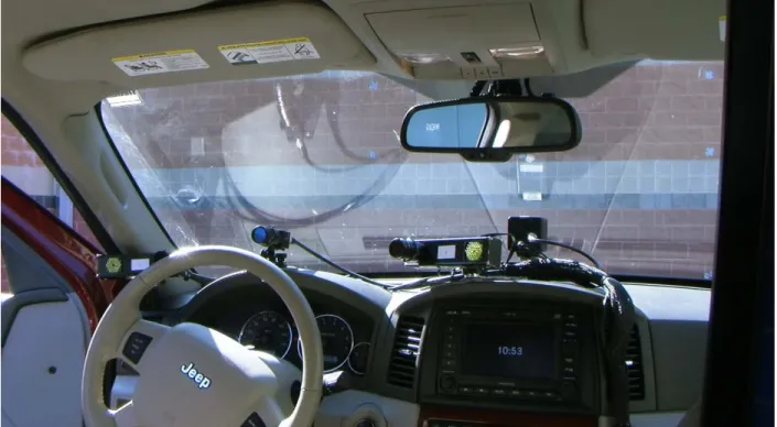
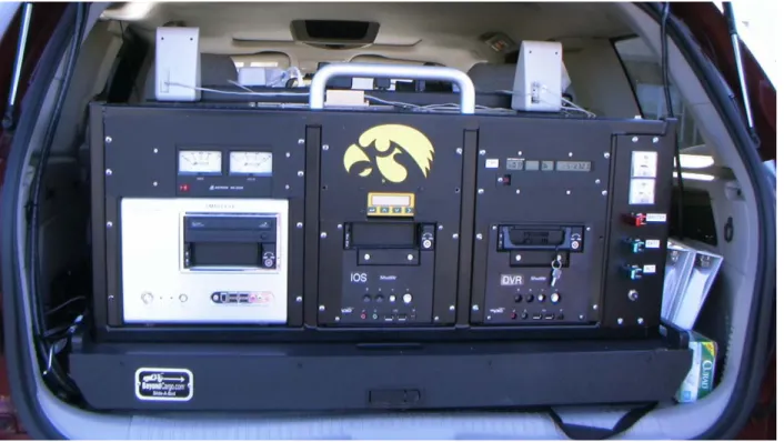
A dash mounted eye tracking device made by SmartEye (a Swedish company) was used to capture drivers’ eye movement, vehicle speed, and other information. The main components of this system consist of two infrared cameras monitoring the driver’s face and eye, 3 outside cameras recording the scenes along the route, and a specialty computer for real time data acquisition and post test information processing. Figures 1, 2, and 3 show the three components of the SmartEye system. The face monitoring units emit infrared beams to the driver’s face and eyes to capture the positions of major face components (ear, nose, and eyes, etc.) and the gaze direction. The system uses a proprietary algorithm to determine the locations of the driver’s fixations. The three scene cameras record forward view at 25 fps. During post processing, images from the three scene cameras are stitched together to create a panoramic scene, and the driver’s eye fixation locations are superimposed onto the stitched images by matching up the synchronized time stamps of the images and text records. The SmartEye system is capable of interfacing with additional device such as GPS unit, accelerometer, and braking sensor, etc. to record additional information. Integration needs to be done by the customer.
Figure 1 Dash mounted infrared cameras
Figure 3 Specialty computer
DATA COLLECTION
Two test routes (Route A and Routed B) were selected from a medium sized city in Southeastern Pennsylvania. The routes contain segments of Expressway, divided and un-divided local roads, and on/exit ramps, etc. Under normal condition, each route would take about 25 minutes to drive through. About 50 drivers of various ages and genders were recruited from the local area. Each driver was given a short orientation, and then asked to drive through Routes A and B as they normally would when driving their own vehicles. The test drives were conducted during non-rush hours in early afternoon, or late evening over the period of one month. The drivers were not told of the purpose of the study, and the eye tracking results can be considered under naturalistic driving condition.
The above field tests were conducted for another propose - to study the possible distraction impact of roadside digital billboards to passing by drivers. This was the first time that FHWA used this type of device to record real time eye tracking data. For various reasons, data for some drivers was not usable or recoverable. The datasets used in this study are associated with 35 test subjects.
DATA REDUCTION APPROACH
Each test subject generated two datasets. A dataset includes all the text and video files generated by the eye trackers after driving through a test route. The system records more than 300 data
elements that include rich information for use by the SmartEye system to determine the driver’s fixations associated with each image. Understanding the meanings of these data elements and being able to use them to investigate the drivers’ visual behaviors would be the most accurate approach. However, it takes time to develop such expertise. In this study, rather than mining through the text files generated by SmartEye, only the eye tracking videos were used, and a computer program was developed to loop through the images in all videos to determine the x and y pixel coordinates of each fixation. A graduate student watched through each video, and manually assigned one of the following road type codes to a range of images:
1. Expressway 2. Divided local road 3. Exit ramp
4. On ramp
5. 4-lane undivided road 6. 2-lane undivided road 7. Other
Any road types not belonging to the 6 explicit categories (including parking lots, intersections, and transition sections from one road to another road, etc.) were coded “Other”. Given that there were limited number of road types on Routes A and B, and on the same segment, the road type was consistent from start to end point, the manual coding process was not very labor intensive. In this study, an image frame is considered a sample (or record). After all samples’ fixation coordinates were computed, their road type values were updated using the manually coded road type values and their GPS speeds were extracted from the text files. Many factors existed could introduce bias into the samples’ visual searching behaviors. To eliminate the bias impacts of some known factors, samples with the following attribute values were eliminated from further analysis:
1. Records without valid fixations.
2. Records with speeds less than 5 mph. Records with this speed range were found at parking lots, intersection stops, or parking on road side for unexpected reasons, etc. 3. Records with speeds greater than 100 mph. This was done to screen out outlier speeds
that might be caused by GPS errors. 4. Records with road type “Other”.
Applying the above screening rules eliminated about half of the total samples. The remaining samples are expected to exhibit more uniform visual search behaviors under given conditions. Table 1 shows the statistical summary of all samples taken from all viewable videos.
Table 1 Statistical Summary of Eye Tracking Data
Day Evening
Number of Unique Datasets 42 29
Total Number of Image Frames (A) 1,656,161 1,080,906
Total Number of Image Frames Without Fixation (B) 522,029 346,192
Overall Dropout Rate (B/A) 31.5% 32.0%
Number of Valid Samples* 851,314 576,518
*: Valid samples are images with fixations that remain after applying screening rules 1 to 4. Analyses results of this study were derived from valid samples.
When working with eye tracking data, data loss is expected. Drivers’ visual searching behavior is temporal and can change instantaneously due to sudden external stimuli. To compensate for the data lose and be able to capture spontaneous changes in gaze direction, eye tracker manufacturers generally resort to larger sampling rate, usually in the order of 50-60 Hz, and up to 1000 Hz.
DATA ANALYSIS APPROACH
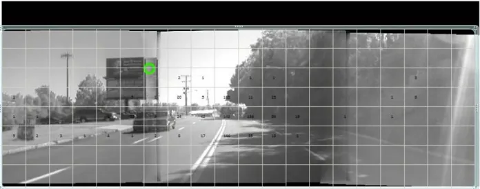
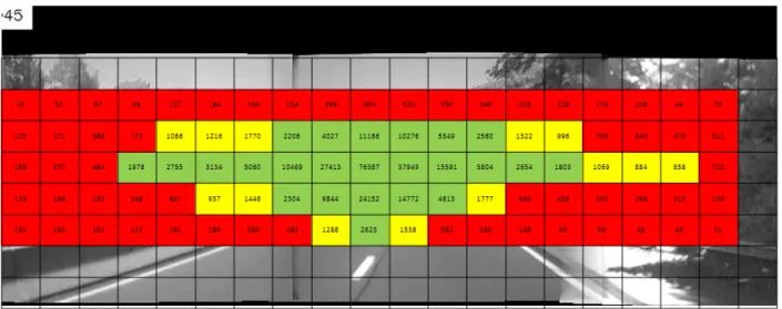
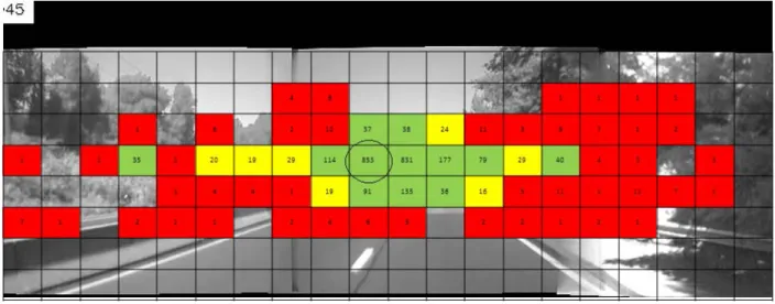
Figure 4 shows a typical image with valid fixation superimposed with a test subject’s fixation pattern. This is an instance of driver visual distraction. The grids shown in Figure 4 are 50 by 50 pixels scaled to the image size. The numbers in the grid cells are the cumulative fixations that a test subject made inside each grid area while driving through this roadway segment. Figure 5 shows the 3-D presentation of the same fixation pattern.
Examining Figures 4 and 5, one can tell that while driving through this segment, the vast majority of the driver’s fixations were in the center area, where attention should be focused on; sparse fixations were found in off-center areas (such as the fixation circle shown in Figure 4) that indicated the driver not paying attention to the driving task (distracted). There are also areas in the image that by just knowing the driver looked at them, we cannot conclude whether or not the driver was distracted.
Although watching the fixations frame by frame can lead to indications of what the driver was looking at, this approach is very tiring to the eyes due to the saccadic nature of eye movements. It also cannot lead to prediction in real time. In this study, we first considered factors that are known to affect the drivers’ visual searching behavior, then devised proper parameters to group the samples into different categories. Next, we studied the features and differences in each fixation pattern, and used them as references to pin point the images that have high likelihood of showing abnormal events or driver distractions.
Figure 4 Typical image with valid fixation superimposed with fixation distribution of associated road type and visibility.
Figure 5 3-D presentation of the fixation pattern shown in previous figure
SAMPL GROUPING DESIGN
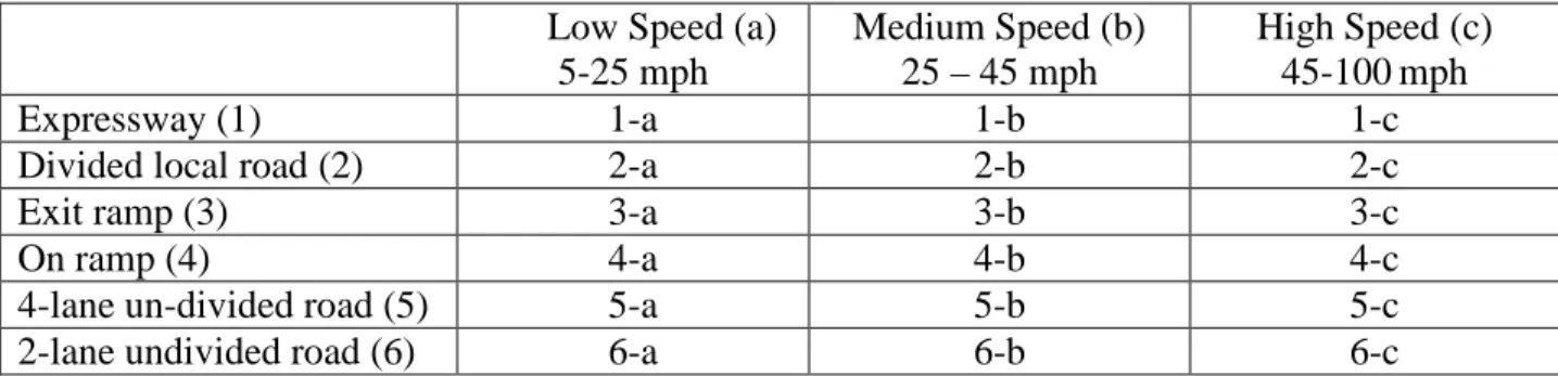
Since all test subjects drove through the same test routes, and each route contained limited number of distinct roadway segments, it is natural to investigate the fixation patterns by road type. We hypothesized that when driving through the same roadway segment, if the speed and visibility conditions vary significantly, drivers would exhibit different visual searching behaviors. Following this thinking process, valid samples were grouped by road types, speed ranges, and visibilities as shown in Table 2, to produce a total of 36 groups.
0 150 300 0 50 100 150 0 50 100150200 250 300 350 400 450500 550 600 650 700 750 800 850 900 950
Table 2 Grouping Designs (Day or Evening) Low Speed (a)
5-25 mph Medium Speed (b) 25 – 45 mph High Speed (c) 45-100mph Expressway (1) 1-a 1-b 1-c
Divided local road (2) 2-a 2-b 2-c
Exit ramp (3) 3-a 3-b 3-c
On ramp (4) 4-a 4-b 4-c
4-lane un-divided road (5) 5-a 5-b 5-c
2-lane undivided road (6) 6-a 6-b 6-c
Note the low, medium, and high speed ranges were defined based on knowledge of the classifications of the roads included.
ANALYSES RESULTS
1. Average Speed and Average Number of Samples
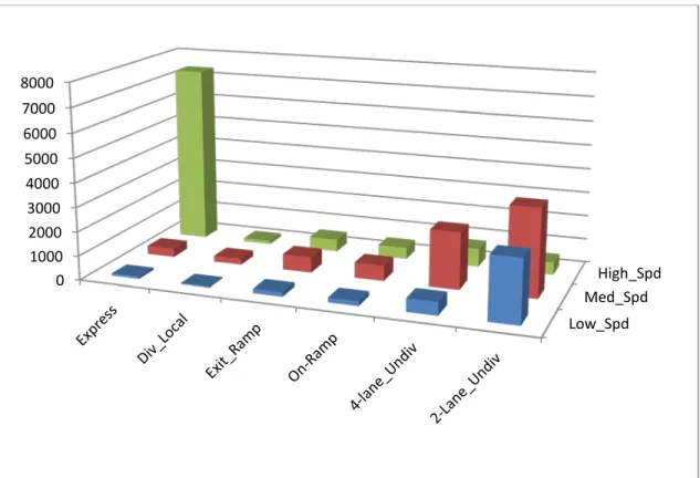
Table 3 shows the average speeds and average number of samples per test subject computed for each group. It shows no visible differences in average speeds exhibited by day and evening samples. The average numbers of valid samples per test subject are plotted in figures 6 and 7, one can see that on higher class road such as Expressway, valid samples concentrated in the higher speed range (> 45 mph); and on lower class roads such as 4-lane and 2-lane undivided roads, valid samples concentrated on medium (25 – 45 mph) and low (5 – 25 mph) speed ranges. These observations make sense and indicate that test subjects were driving at the appropriate speeds when passing through different roadway segments.
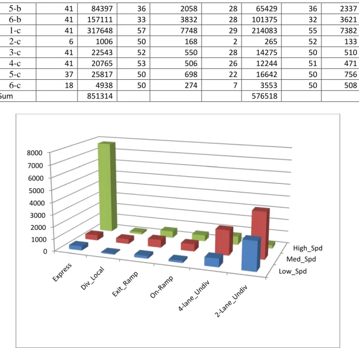
Table 3 Average Speeds and Average Number of Samples per Test Subject Case Scenario Day Evening Num of Unique Test Subjects Total Num of Samples Avg Speed (mph) Avg Num of Samples per Subject Num of Unique Test Subjects Total Num of Samples Avg Speed (mph) Avg Num of Samples per Test Subject 1-a 8 2783 15 348 10 926 15 93 2-a 20 1577 20 79 12 520 21 43 3-a 41 9072 16 221 26 4661 16 179 4-a 40 6923 21 173 28 5334 22 191 5-a 41 28167 16 687 28 15217 16 543 6-a 41 97277 17 2373 28 71996 17 2571 1-b 29 12832 39 442 27 9632 40 357 2-b 19 7619 36 401 14 3466 36 248 3-b 41 26838 37 655 28 18345 37 655 4-b 40 24001 32 600 29 18555 32 640
5-b 41 84397 36 2058 28 65429 36 2337 6-b 41 157111 33 3832 28 101375 32 3621 1-c 41 317648 57 7748 29 214083 55 7382 2-c 6 1006 50 168 2 265 52 133 3-c 41 22543 52 550 28 14275 50 510 4-c 41 20765 53 506 26 12244 51 471 5-c 37 25817 50 698 22 16642 50 756 6-c 18 4938 50 274 7 3553 50 508 Sum 851314 576518
Figure 6 Average numbers of samples per test subject - Day
Low_Spd Med_Spd High_Spd 0 1000 2000 3000 4000 5000 6000 7000 8000
Figure 7 Average numbers of samples per test subject – Evening 2. Fixation Patterns
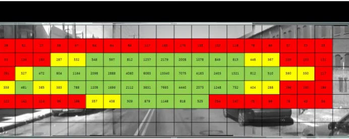
As explained, Figures 4 and 5 show a driver’s visual fixation pattern for the case scenario of medium speed, 4-lane undivided road under day time visibility. Although they are intuitive in revealing the visual searching patterns, our research indicated that the numbers in corresponding grid cells between different groups were not suitable for direct comparisons. What seemed consistently comparable were the shape, location, and area of the horizontal cross-section of the cone shown in Figure 5. To make it intuitive when comparing the fixation patterns between different groups, the following operations were made to each fixation matrix:
1. Rank the numbers in the fixation matrix (refer to Figure 4) in descending order.
2. Divide the ranked numbers by the total number of fixations in that group to get the percentage ranking of each data element.
3. Compute the cumulative percentage of each ranked data element.
4. Color all grid cells with cumulative percent values of [0%, 90%) with light green color. 5. Color all grid cells with cumulative percent values of [90%, 95%) with yellow color. 6. Color all grid cells with cumulative percent values of [95%, 100%] with red color.
Figures 8 and 9 show the color coded fixation patterns of High Speed-Expressway-Day, and High Speed-Expressway-Evening groups. In this study, we associate fixations onto the light
Low_Spd Med_Spd High_Spd 0 1000 2000 3000 4000 5000 6000 7000 8000
green, yellow, and red colored areas with instances of driver attention, possible distraction, and definite distraction. When examining the color coded areas, one may visualize the fixations as a pile of beans with 90% of them piled up in the light green area, 5% spread in the yellow area, and the remaining 5% scattered in the red area.
Figure 8 Fixation pattern associated with High Speed-Expressway-Day group
Figure 9 Fixation pattern associated with High Speed-Expressway-Evening
Comparing Figures 8 and 9, one can see that the light green area of Figure 9 is much smaller and also lower, meaning on the same roadway segment and under the same speed, drivers tended to look toward the center (more concentrated on driving task), and at closer distance under dark condition. This conforms to expectation.
Figures 10 and 11 show the fixation patterns of Low Speed-2 lane undivided roadway-Day, and High Speed-2 Lane undivided roadway-Day. Comparing them, one can see that as speed got
higher, drivers looked more towards the center (paid more attention to driving task). This again conforms to expectation.
Figure 10 Fixation pattern associated with Low Speed–2 lane undivided road-Day
Figure 11 Fixation pattern associated with High Speed – 2 lane undivided road – Day Figure 12 shows the fixation pattern of Low Speed-Expressway-Day. Comparing it with the fixation pattern of High Speed-Expressway-Day (Figure 8), the light green area in Figure 12 is more concentrated in the center, indicating drivers were paying more attention to the driving task at lower speed. This seems contrary to the expectation that drivers should be more relaxed when driving at lower speeds, and indicates possible abnormal events might be happening then.
To verify the observation, all records with fixations onto the grid cell marked in Figure 12 were extracted from the Low-Speed-Expressway-Day group. There were 853 records associated with 8 unique test subjects, the frame ranges associated with each test subject were sequential and seemed continuous. After viewing the videos associated with these 8 events, it was found that
four events happened at exactly the same location as shown in Figure 13, the merging location of an on ramp and the expressway. In two events, the test subjects slowed down waiting for
vehicles from the adjacent expressway through lane to pass through before entering the expressway, in other two events, one showed a car in front of the test vehicle waiting on the ramp, and the other showed traffic on the expressway and a police car parked on the shoulder downstream of the ramp. The frames identified were on the expressway, but the events actually started from the on ramp. The video clips indicated that the acceleration lane of this on ramp may not be long enough.
Figure 12 Fixation pattern associated with Low Speed –Expressway –Day
Figure 13 Low Speed-Expressway-Day abnormal event (speed too low). Reason: other car stopped in front waiting for gap to enter the expressway from on ramp.
Of the remaining 4 events, one showed the test vehicle getting closer to congested traffic and slowed down, one showed a rainy day with cars in front and side, one showed an SUV applying
brake in front of the test vehicle, and one showed no car in front, but the sun was shining through the windshields as shown in Figure 14, and apparently impaired the driver’s vision temporarily.
Figure 14 Low Speed-Expressway-Day abnormal event (speed too low). Reason: sunshine.
Figures 15 and 16 show the fixation patterns of High Speed-On Ramp-Day, and High-Speed-On Ramp-Evening. The light green area in Figure 16 is smaller and towards the center, indicating drivers focused more on the driving task when entering the expressway under high speed in the evenings, which is expected. However, both Figures show yellow areas at the lower left corner, as circled in Figures 15, and 16, that seem strange and deserve further investigation.
Figure 16 Fixation pattern associated with High-Speed – On Ramp – Evening
Records with fixations onto the circled areas indicated in Figures 15 and 16 were extracted from the associated groups and examined. It was found that for the day group, there were 30 events associated 25 test subjects; and for the evening group, there were 25 events associated with 13 test subjects. All events were brief, most had 1 to 5 fixations in the circled areas, and they happened either before two lane merging into one lane in the middle of on ramp, or before entering the expressway. Almost all events (day or evening) occurred in the middle of on ramp were associated with the location shown in Figure 17, a long on ramp merging from 2 lanes into one lane. The videos showed that in all but two instances, the test vehicle was driving on the right lane under high speed preparing for the upcoming merge. Under the given circumstance, the visual searching patterns exhibited by the test subjects were appropriate and these events were not distractions.
The analysis results presented thus far demonstrated the capability of the proposed methodology in identifying abnormal events, driver visual distractions, locations of (merging) conflicts, and locations that require the driver to look at specific areas under given circumstance. For any fixation pattern, the number of events associated with any grid cell can be as many as the number of datasets (videos) in that group. Examining identified events must be done manually by watching portions of the videos that contain the identified frame ranges. Due to space limitation, it is not practical to present the analysis results of all 36 groups.
DISCUSSIONS
In this study, fixations onto the red cells were considered instances of definite visual distraction. By virtual of the way grid cells were colored, fixations onto the un-colored grid cells would also be considered instances of visual distraction if the fixation patterns were used as reference in real time. In is commonly agreed in the research community that glancing away from the forward roadway for 2 seconds or longer would present a significant crash risk. Knowing that the eye tracker’s sampling rate was 50 Hz, the scene cameras’ recording rate was 25fps, and the overall fixation dropout rate was 32%, 2 seconds continuous visual distraction would be about 34 fixations onto the red or un-colored grid cells by the same test subject within 100 timestamp increments. Using the proposed methodology, hundreds of visual distraction instances can be identified by simply picking out the samples with fixations onto the red colored cells. Exactly how many instances were visual distraction events of 2 seconds or longer need to be examined manually by watching relevant videos. That work is not complete as of this writing.
In the grouping design, we used the same low, medium, and high speed ranges for all types of roadway segments. It is probably more appropriate to use different ranges of low, medium, and high speeds for different roadways by considering their posted speed limits. Similarly, we used the same cumulative percent fixations of 0%-90%, 90%-95%, and 95%-100% as color coding thresholds for all case scenarios. Experience tells us that there are factors such as congested traffic, bad weather, and poor visibility, etc. that can prompt the drivers to look more towards center, under those circumstances, the cumulative percent thresholds should be adjusted. These two types of sensitivity analyses are major efforts by themselves, and we haven’t had the resource to investigate them. For the analyses completed thus far, the grouping and color coding parameters used did produce high success rate (over 90%) in guiding us to identify abnormal events or driver distractions. The results presented are sufficient to demonstrate how the methodology works.
The abnormal events identified in this study can be considered near events that could lead to crashes if the drivers didn’t slow down or looked at the locations indicated in Figures 12, 15, and 16 under given circumstances. These events stood out naturally through the analysis process due to their attribute values in contrast with other samples. Most of the events identified might not
be noticeable if one just watched the videos because were no evasive steering observed, and events were too brief to catch the observer’s attention.
The datasets were collected from 35 test subjects, each drove through 2 test routes. The same amount of data could also be accumulated by a single driver after 36 hours of driving. In theory, fixation pattern can be developed for any type of roads; for the same segment, fixation patterns can be further developed by travel direction and time of the day periods. Assuming there is an eye tracker and a GPS unit installed in the vehicle and the fixation patterns for each roadway segment (by direction and time of the day periods) have been accurately determined, the proposed methodology can be used in real time to detect instances of abnormal events or driver distractions, and provide proper warnings to alert the driver.
When designing the field experiments, principles in statistical design and human factor design were considered to ensure the test subjects represent the desired spread in ages and genders; the routes included enough number of digital and static billboards; and the tests be done during low traffic hours and reflected day and evening visibilities. In this study, we used the same datasets, took great care in eliminating samples that might introduce bias into the visual search patterns, and defined grouping parameters aimed at improving uniformity of samples’ visual searching patterns in each group. The analyses done so far are qualitative and serve in part to validate proposed methodology. Once the fixation patterns are confirmed, analytical tools dealing with spatial distribution can be used to differentiate the fixation patterns.
Certain roadway features such as sharp curves and steep grades, etc., require the driver to look at specific off-center areas towards the left/right or up/down in the field of view, and special roadway categories may be defined for them. In this study, we defined on ramp and exit ramp as specific categories, both included curves and grades; we eliminated records with road type coded as “Other”, which included transition sections from one road to another road that often were curves. However, we didn’t examine the curves and grades that might exist in the middle of a segment. Moderate curves and grades are not expected to alter the fixation patterns. If a roadway segment is mostly tangent, but contains one sharp curve/steep grade in the middle somewhere that would cause the drivers to concentrate fixations onto a small area, and slow down significantly, we expect the proposed methodology can identify the events associated with passing though the curve/slope, recall how we identified the abnormal events associated with low speed expressway, and the glancing events associated with high speed on ramp groups.
CONCLUSIONS
1. The grouping criteria and color coding parameters used in this study produced satisfactory results in guiding the analysis process. When resource permits, sensitivity analysis on grouping by speeds, and color coding thresholds should be performed to
accurately reflect field conditions. The grouping process alone can lead to the identification of some abnormal events.
2. The fixation patterns developed reveal drivers’ predominate visual searching patterns associated with specific types of roadways under given speed and visibility conditions; they confirmed the expectation that drivers tend to look more toward the center of field of view when attention demanding loads increase (such as higher speed, poorer visibility, and approaching congested traffic, etc.).
3. The proposed methodology is effective in isolating out records with specific attribute values that deserve further investigation, which may lead to the identification of abnormal events, or validating drivers’ visual searching pattern when approaching specific roadway features; it is also capable of spotting locations of special roadway features that require the driver to slow down and look at specific off-center areas.
4. Additional road types such as sharp curves and steep grades may be introduced to investigate driver visual behaviors specific to those roadway features. There is tradeoff between the number of groups needed and the statistical significance desired in each group.
5. The analyses done in this study are exploratory in nature to test the effectiveness of the proposed methodology. More elaborate analytical tools dealing with spatial distribution can be used to model the fixation patterns associated with different case scenarios.
REFERENCES
NTHSA (2009), An Examination of Driver Distraction as Recorded in NTHSA Databases. Research No. DOT HS 811 216.
Chapman, P.R. and Underwood, G. (1999). Looking for danger: Drivers’ eye movements in hazardous situations. In A.G. Gale et al. (Eds.) Vision In Vehicles (pp. 527-532). U.K.: Taylor & Francis.
Yarbus A. (1967). Eye Movements and Vision. Translated from the Russian edition (Moscow, 1965) by Basil Haigh. Lorrin A. Riggs, Translation Ed. Plenum, New York, 1967.
Zwahlen, H. T., Russ A., and Schnell, T.(2003). TRB 2003 Annual Meeting CD-ROM. Driver Eye Scanning Behavior While Viewing Ground-Mounted Diagrammatic Guide Signs before Entrance Ramps at Night.
Eizenman, M. Jares, T. and Smiley, A. (1999). A new methodology for the analysis of eye-movements and visual scanning in drivers. Transport Canada Contract report. March 1999. Barbluk, J.L., Noy, Y.I., and Eizenman, M. (2002). Impact of Cognitive Distraction on Driver Visual Behavior and Vehicle Control. Transport Canada, TP# 13889.
Tijerina, L, Barickman, F. S. and Mazzae E. N. (2004). Driver Eye Glance Behavior During Car Following.U.S. DOT and NTSHA,Report Number: DOT HS 809 723.