Estimating Causal Effects from Nonparanormal Observational Data

University of Groningen

Estimating Causal Effects from Nonparanormal Observational Data

Mahmoudi, Seyed Mandi; Wit, Ernst C.

Published in:

The international journal of biostatistics

DOI:

10.1515/ijb-2018-0030

IMPORTANT NOTE: You are advised to consult the publisher's version (publisher's PDF) if you wish to cite from it. Please check the document version below.

Document Version

Final author's version (accepted by publisher, after peer review)

Publication date: 2018

Link to publication in University of Groningen/UMCG research database

Citation for published version (APA):

Mahmoudi, S. M., & Wit, E. C. (2018). Estimating Causal Effects from Nonparanormal Observational Data. The international journal of biostatistics, 14(2), [20180030]. https://doi.org/10.1515/ijb-2018-0030

Copyright

Other than for strictly personal use, it is not permitted to download or to forward/distribute the text or part of it without the consent of the author(s) and/or copyright holder(s), unless the work is under an open content license (like Creative Commons).

Take-down policy

If you believe that this document breaches copyright please contact us providing details, and we will remove access to the work immediately and investigate your claim.

Downloaded from the University of Groningen/UMCG research database (Pure): http://www.rug.nl/research/portal. For technical reasons the number of authors shown on this cover page is limited to 10 maximum.

Estimating Causal Effects from Nonparanormal

Observational Data

Seyed Mahdi Mahmoudi1_{, Ernst C. Wit}2

1_{Department of Statistics, Semnan University, Iran, E-mail:}

[email protected]

2_{Bernoulli Institute, University of Groningen, Netherlands, Email:}

[email protected] 19 June, 2018

Abstract

One of the basic aims of science is to unravel the chain of cause and ef-fect of particular systems. Especially for large systems, this can be a daunting task. Detailed interventional and randomized data sampling approaches can be used to resolve the causality question, but for many systems, such inter-ventions are impossible or too costly to obtain. Recently, Maathuis et al. (2010), following ideas from Spirtes et al. (2000), introduced a framework to estimate causal effects in large scale Gaussian systems. By describing the causal network as a directed acyclic graph it is a possible to estimate a class of Markov equivalent systems that describe the underlying causal interac-tions consistently, even for non-Gaussian systems. In these systems, causal effects stop being linear and cannot be described any more by a single coef-ficient. In this paper, we derive the general functional form of a causal effect in a large subclass of non-Gaussian distributions, called the non-paranormal. We also derive a convenient approximation, which can be used effectively in estimation. We show that the estimate is consistent under certain conditions and we apply the method to an observational gene expression dataset of the Arabidopsis thaliana circadian clock system.

1

Introduction

Inferring cause-and-effect relationships between variables is of primary importance in many fields of science. The classical approach for determining such relation-ships uses randomized experiments where a single or few variables are perturbed.

Such intervention experiments, however, can be very expensive, unethical (e.g. one cannot force a randomly selected person to smoke many cigarettes a day) or even infeasible. Hence, it is desirable to infer causal effects from so-called observa-tional data obtained by observing a system without subjecting it to interventions. Although some important concepts and ideas have been worked out (Spirtes, Meek, and Richardson, 1995, Richardson, 1996, Mooij, Janzing, Heskes, and Sch¨olkopf, 2011), estimating causal effects for non-Gaussian observational systems is still in its infancy.

Pearl (1995, 2009) described a do-calculus of causal effects, if the underlying causal diagram is known. In practice, though, the influence diagram is often not known and one would like to infer causal effects from observational data together with the influence diagram. Spirtes, Glymour, and Scheines (2000) introduced methods to estimate causal graphs from observational data. Verma and Pearl (1990) found that typically groups of causal graphs give rise to the same distribution of the data, which implies that the generating causal DAG is typically unidentifiable from the data. This Markov equivalence class of causal DAGs has been called completed partially directed acyclic graph (CPDAG). A CPDAG can be estimated in various ways, including the PC-algorithm (Spirtes et al., 2000), search and score methods (Chickering, 2002, 2003, Verma and Pearl, 1990) and Bayesian methods (Hecker-man and Geiger, 1995, Spiegelhalter, Dawid, Lauritzen, and Cowell, 1993).

The PC-algorithm uses conditional independence tests to infer a CPDAG from data (Spirtes et al., 2000). Sample partial correlations derived from independent multivariate normal observations have favourable distributional properties (Ander-son, 2003, Chapter 4), which form the basis for the work of Kalisch and B¨uhlmann (2007), who treat the PC-algorithm in the Gaussian context with conditional inde-pendence tests based on sample partial correlations. They prove the high-dimensional consistency of the PC-algorithm, when the observations form a sample of indepen-dent normal random vectors that are faithful to a suitably sparse DAG. Maathuis, Kalisch, and B¨uhlmann (2009) propose a method that combines the estimation of the causal structure and the interventional distribution in the Gaussian case. Due to the Gaussian structure, they find that the causal effects can be described by a set of regression coefficients. Harris and Drton (2013) show that the PC-algorithm has high-dimensional consistency properties for a broader class of distributions, when standard Pearson-type empirical correlations are replaced by rank-based measures of correlations in tests of conditional independence, such as Spearman’s rank cor-relation and Kendall’s tau. A special class of non-Gaussian distributions is consti-tuted by the Gaussian copula, or, in the terminology of Liu, Han, Yuan, Lafferty, and Wasserman (2012), the so-called “nonparanormal distributions.” Teramoto, Saito, and Funahashi (2014) uses this class to estimate the underlying causal DAG for the design of efficient intervention experiments. Nandy, Maathuis, and

Richard-son (2017) appliedIntervention-calculus when the DAG is Absent (IDA) to

non-paranormal distributions, and summarize the causal effects among the underlying Gaussian random variables. What is missing up until now is a way to describe and estimate the causal effects in such nonparanormal scenarios. The main difficulty is that causal effects in non-Gaussian scenarios stop being constant and become functions of the intervention variables.

In the remainder of the paper, we will consider an observational setting of a nonparanormal system. We assume the causal CPDAG has been estimated by, e.g., the Rank PC (RPC) algorithm (Harris and Drton, 2013), i.e., the PC-algorithm in the nonparanormal context. Based on the estimated CPDAG, it is our aim to derive an expression for the causal effect in this system and to find a consistent way to estimate them. In section 2, we introduce the causal graph terminology, a short description of the intervention calculus and the definition of a causal effect. In section 3, we derive the structure of a causal effect of a nonparanormal causal effect and in section 4, we define a convenient estimator. In section 5, we evaluate the performance of our method in a simulation study. Finally, in section 6, we illustrate the method in a real data example.

2

Causal effects in causal graphs

In this section we describe the background needed in order to define the notion of a causal effect. We begin by defining causal models through directed graphical models.

Agraphis a pairG= (V,E), whereVis a finite set ofvertices V={1,2, . . . ,p},

also callednodes, ofGandE is a subset of(V×V)of ordered pairs of vertices,

called theedgesorlinksofG. We consider prandom variablesX1, . . . ,Xp,

associ-ated to the vertices. If edge(Xi,Xj)∈Ebut(Xj,Xi)∈/E, we call the edgedirected

or anarrow, denoted byXi →Xj. In that case, we also say thatXi is a parentof

Xj, and that Xj is a child ofXi. The set of parents of a vertex Xj is denoted by

pa(j). We use the short-hand notationXi Xj that isundirected edge to denote (Xi,Xj)∈E and(Xj,Xi)∈E. A graph containing only directed edges (→) is

di-rected, one containing only undirected edges ( ) isundirected. A directed graph

is called adirected acyclic graph(DAG) if it does not contain directed cycles. A

DAG of p random variables X1, . . . ,Xp can be interpreted as a Markov

indepen-dence graph, describing a multivariate distribution. Various DAGs can lead to the same distribution. A common tool for describing such Markov equivalence class of DAGs are completed partially directed acyclic graphs (CPDAGs).

Pearl (2009) defined causality through intervention, whereby variables are ex-ternally manipulated to take certain values. This intervention changes the

under-lying distributionP and can be expressed by adapting the DAG. The new

distri-bution is called theintervention distributionand we say that the variables, whose

structural equations we have replaced have been “intervened on.” The intervention distribution ofY when doing an intervention and setting the variableXi to a value

x0_i is denoted by P(Y|do(Xi=x0i)). The intervention on variable Xi is

character-ized by atruncated factorization, in which an intervention DAGG0, arising from

the non-intervention DAGGcan be defined by deleting all edges which point into

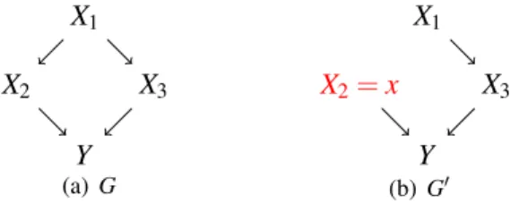
the nodeXi. Consider the example graph below, a DAGGand its corresponding

intervention graphs (G0) are shown. X1 X2 X3 Y (a)G X1 X2=x X3 Y (b)G0

Figure 1: (a) A DAG G and (b) its corresponding intervention graph G0. The

intervention is do(X₂=x), described by the red label in the graph. The parental set

ofi=2 is pa(2) ={1}which appears in (3) for computing the causal effectβ2of X2onY.

Thetotal causal effect ofXi onY atxi is the relative amountY is expected to

change as a result from a smallinterventionalchange ofXiatxi,

CE(Y|Xi=xi) = ∂

∂xE[Y|do(Xi=x)]|x=xi, (1)

where we have that ifY ∈/X_pa(i),

E(Y|do(Xi=x)) = Z

E(Y|Xi=x,Xpa(i)=xpa(i))P(xpa(i))d(xpa(i)). (2)

If(X1, ...,Xp−1,Y)has a multivariate Gaussian distribution, then using the fact that

the conditional expectationE(Y|Xi =x,Xpa(i)=xpa(i)) is linear in xi andxpa(i) if

Y ∈/X_pa(i), it is straightforward to see that

E(Y|_do(Xi=xi)) =βixi+

Z

β_paT_(i)x_pa(i)P(xpa(i))d(xpa(i)),

for some coefficientsβiandβpa(i). Therefore, the causal effect is given by

CE(Y|Xi=xi) = ∂

From (3), it follows that the total causal effect ofXi onY withY ∈/Xpa(i)is given

by the regression coefficient ofXiin the regression ofY onXiand pa(i). Note that

ifY ∈X_pa(i), the total causal effect fromXi toY is, obviously, zero. Our aim is to

generalize this to a wider class of distributions.

3

Causal effect for nonparanormal graphical models

Spirtes et al. (2000) introduced the PC-algorithm to estimate causal graph from observational data. Kalisch and B¨uhlmann (2007) proved consistency of the PC-algorithm in a Gaussian setting for estimating the causal skeleton and, subse-quently, the Markov equivalence class of high-dimensional causal graphs. The algorithm is based on a clever hierarchical scheme for testing conditional inde-pendence among pairs of variablesXj,Xk (for all j6=k) in the DAG. In Gaussian

models, tests of conditional independence can be based on Pearson correlations and high-dimensional consistency results have been obtained for the PC-algorithm in this setting. Harris and Drton (2013) proved high-dimensional consistency prop-erties for a broader class of nonparanormal models when using rank-based mea-sures of correlation. They showed that the Rank PC-algorithm (RPC) works as

well as the Pearson PC-algorithm for normal data and considerably better for non-Gaussian data. If one assumes to know all conditional independencies exactly – the oracle setting– then the RPC-algorithm yields the “true” CPDAG, i.e., the Markov equivalence class of DAGs that contains the true causal DAG.

Building on this work in the Gaussian setting, Maathuis et al. (2009) derived an expression for and an estimator of the total causal effect of a covariateXi on

a responseY in a Gaussian causal graph. After obtaining the CPDAG Markov

equivalence class of, say, m causal DAGs, they apply for each DAG Gj in this

class the intervention calculus to obtain the total causal effectβi jofXionY. Then

they define multi-setsΘi={βi j}j∈{1,...,m}containing the estimated possible causal

effects ofXionY.

In this section, we derive the analogous multi-set of causal effects the nonpara-normalsetting. In practice, the conditional independences have to be inferred from

the data as well and we show how using our main result in combination with the RPC-algorithm we are able to define an convenient estimator for the causal effect for such data, which stops being linear and needs to be estimated functionally.

3.1 General expression of nonparanormal causal effect

Liu et al. (2012) define the nonparanormal distribution. Let f= (fi)i∈Vbe a set of

matrix. We say ap-dimensional random variableX= (X₁, ...,Xp)Thas a

nonpara-normal distribution,

X ∼NPN(µ,Σ,f),

if f−1(X) = (f₁−1(X₁), . . . ,f_p−1(Xp))∼N(µ,Σ). IfX∼NPN(µ,Σ,f), then the

uni-variate marginal distribution for a coordinate, sayXi, can have any distributionFi,

as we can take fi=F_i−1◦Φ_µi,σ2

i , whereΦµi,σi2 is the normal distribution function

with meanµi and varianceσi2=Σii. Note that, in general, fi need not be

contin-uous. However, in this paper, we deal with monotone and differentiable f. Liu

et al. (2012) show that in that case the nonparanormal distribution NPN(µ,Σ,f)is

a Gaussian copula.

In the remainder of the paper, we assume that(X1, . . . ,Xp−1,Y)∼NPN(0,Σ,f),

where Σ is a correlation matrix. We will refer to the latent standard normally

distributed variables asZi=fi−1(Xi) =Φ−1◦Fi(Xi)andZ=fy−1(Y) =Φ−1◦Fy(Y).

We are interested in the total causal effect ofXi onY for i∈(1, . . . ,p−1). We

know from section 2 that for Gaussian data it is very simple to compute the total causal effect, since Gaussianity implies thatE(Y|Xi =xi;X−i =x−i) is linear in xi. Unfortunately, this is no longer true for non-Gaussian random variables. In

Theorem 1 we derive the explicit functional form for the total causal effect in the entire class of nonparanormal distributions.

Theorem 1. Let(X1, . . . ,Xp−1,Y)∼NPN(0,Σ,f) and fi (i=1, . . . ,p−1)is

dif-ferentiable and fyis infinitely differentiable, then the total causal effect of Xi on Y

in causal graph G is given by CE(Y|Xi=xi) = ∞

∑

∑

∑

for every z0 ∈R, where fy(k) is the kth derivative of fy, zi = f_i−1(xi), Zpa(i) =

f_pa−1_(i)(Xpa(i)),(βi,βpa(i)) =Σp,(i,pa(i))Σ₍−i,1pa(i)),(i,pa(i))andρ= (βi,βpa(i))Σ(i,pa(i)),p.

The proof of the theorem is given in the appendix. We have obtained the gen-eral expression (4) for a nonparanormal causal effect. The value of this theorem is that it gives us insight in how higher order moments of the effectY, captured

in the higher order derivatives of fy, affect the causal effect, whereas higher order

moments of the causeXi do not. In practice, this formula is not very helpful as

the correlation structure of the latent normal variable. However, this formula can inspire practical estimation procedures of the causal effects in nonparanormal sys-tems. Whereas this is in principle possible, we restrict our attention in this paper to a lower order Taylor approximations. A first and second order Taylor expansion are given by CE_1,z0(Y|Xi=xi) = fy0(z0)βi(f −1 i ) 0 (xi), CE_2,z0(Y|Xi=xi) = f_y0(z₀)βi+fy00(z0)βi(βizi−z0) ×(f_i−1)0(xi).

If median and mode ofY coincide, then it is easy to show that the second order

Taylor expansion collapses to the first order by takingz0=0, i.e.,CE2,0(Y|Xi=

xi) = (F−1)0(0.5)βi(f_i−1)0(xi). Higher order expansions become quickly more

in-tricate. Moreover, especially when it comes to estimation in section 4, the estimates involved in lower order expansions tend to be intrinsically more stable.

3.2 Special case

We consider the special case of the above theorem for the situation that onlyY is

normally distributed, and theXis are still nonparanormal.

Corollary 1. Let(X1, . . . ,Xp−1)∼NPN(0,Σ,f)and fi (i=1, . . . ,p−1)is

differ-entiable and Y ∼N(µ,σ2), then the total causal effect of Xi on Y in causal graph

G is given by

CE(Y|Xi=xi) =σ βi(fi−1)

0

(xi), (5)

whereβiis defined as in Theorem 1.

The result simply follows from fy(Z) =µ+σZ for Z standard normal. This

special case both inspires an estimator for the causal effect and gives some hope for obtaining some consistency results.

4

NCE: nonparanormal causal effect estimator

In this section, we propose a simple estimator for the causal effect that is able to capture non-linear effects for a wide-ranging collection of distributions. Further-more, we show that under some conditions, this estimator is consistent.

0.5 1 0 Y Xi 0 d F_Y,−1_sm ∂ ∂uFd− 1 Y,sm|u=0.5 (a) (b) xi ∂ ∂xFbi,sm|x=xi 1 d F_Y,−1_emp

Figure 2: (a) the derivative of monotone increasing spline_F[−1

Y,smfor estimate∂∂xF

−1

Y .

(b) the derivative of the monotone increasing estimating splineFbi,sm for estimate ∂

∂xFi.

4.1 First order estimator

In section 3.2, we derived a one-term expression that is used as inspiration for a first-order Taylor estimator of the general causal effect ofXi=xonY, i.e.,

d

NCEz₀(x) = fˆy0(z0)βˆi(dfi−1)

0₍

x), (6)

for somez0, x∈Rand where ˆβi is the linear regression coefficient of dfy−1(Y)on

d_f−1

i (Xi), while controlling for the parents fd

−1

pa(i)(Xpa(i))ofi, given some estimators

for the various functions f−1and fy. We will show in the next section that in order

to obtain consistency, we trim the data for each variable below itsα/pand above

1−α/p quantiles, where pis the number of random variables(X,Y). When an

observation has been trimmed for one variable, it is removed in its entirety for all variables. This means that in the worst case scenario, 1−₂α of the observations

remain. In practice, we will often useα =0.05.

it is straightforward to obtain f_y0(0) = ∂ ∂uF −1 Y (u)|u=0.5φ(0) (f_i−1)0(x) =φ(f_i−1(x))−1 ∂ ∂xFi(x),

where φ is the density function of a standard normal distribution. Considering

Figure 2,F_Y−1 will be estimated via a monotone increasing smootherF[_Y−_,sm1 , which

gives us direct access to its derivative. Similarly, ∂

∂xFi will be estimated by

tak-ing the derivative of the monotone increastak-ing estimattak-ing smootherFbi,sm. Finally,

f_i−1(x)will be estimated as ˆz=Φ−1(Fˆi,sm(x)). Putting this together, we obtain a

simplified and explicit estimator of a non-paranormal causal effect, d NCE0(x) =βˆi φ(0) φ(zˆ) ∂F[_Y−_,sm1 ∂u (0.5) ∂Fbi,sm ∂x (x). (7)

In the following section, we will show that under certain conditions the above estimator is consistent. In particular, we show that estimatingF_Y−1 andFi with a

particular kind of kernel smoother works. Nevertheless, in practice any slightly stiff smoother will result in almost the same estimates. A natural cubic spline is easy to implement and can be easily differentiated, which is needed for the causal effect estimator_NCEd₀(x).

4.2 Consistency

In this section we will be concerned with the asymptotic behaviour of our esti-mator in (7) under the assumption of normality ofY, but no such assumption on

theXi. We first show that the random, but not necessarily independent, sampling

scheme of(X₁, . . . ,Xp−1)∼NPN(0,Σ,f) andY ∼N(µ,σ2) combined with our

lower and upperα/ptrimming scheme will eventually fill up the p-dimensional

cube[Lα,Uα], whereLα= (Lα1, . . . ,L p−1 α ,L y α)andUα= (Uα1, . . . ,U p−1 α ,U y α)are the α- and(1−α)-quantiles , respectively, for each of the variables(X1, . . . ,Xp−1,Y).

From the original sample sizen approximately(1−2α)n will fall in this cube.

Then we show that the kernel estimators of the functions used in the NCE estima-tors and their derivatives converge fast to their true values in probability. Together with the fact that products of consistent estimators are consistent, this proves the consistency of the estimator_NCEd₀(x).

Proposition 1. Consider any absolutely continuous random variable X with lower

α quantile Lαand upperα quantile Uα. For the N(1−2α)n ordered

observa-tions of X in the finite interval[Lα,Uα], the following property holds

max

2≤i≤N|X(i)−X(i−1)|=OP(1/N).

The symboldenotes that two sequences of real numbers are asymptotically of

the same order. The proof of this Proposition is a simple exercise and will not be given here.

Our goal is first to estimate the functionFi and its derivative _∂∂_xFi. Similarly,

we aim to estimateF_i−1and its derivative. In order to derive asymptotic properties,

we will be using kernel estimators for ˆFi,smandFd_i,−_sm1(x), respectively,

ˆ Fi,n(x) = N

∑

∑

forx∈[Li_α,U_αi]andu∈[α,1−α], where K is a kernel function, (Priestley and

Chao, 1972),bn>0 denotes the bandwidth that we take to depend on the sample

sizenin such a way thatbn→0 asn→∞andxi(1),xi(2), . . . ,xi(N)denote the

or-der statistics of that part that for theivariable that falls within[Li_α,U_αi]. Note that

we have selected the same bandwidth for the quantile function and the CDF, even though they could live on completely different domains. In practice, it may be sen-sible to scale the bandwidth by some constant depending on the domain. However, for proving consistency we do not need it. We define an estimator of ∂

∂xFiby taking

the derivative of the kernel smoother [∂

∂xFi,n=

∂

∂xFˆi,n=Fˆ

0

i,n.

Proposition 2. If the kernel K is symmetric and twice continuously differentiable

with support in[−1,1]and if it satisfies the integrability conditions (a)R₋1₁K(u)du=

1and (b)R₋1₁u`K(u)du=0 for`=1, . . . ,γ−1, then for a fixed numberδ,such

thatα <δ <1/2 :

(i) if F and F−1 are γ ≥1 times continuously differentiable and bn→ 0 as

n→∞,then sup x∈[Li α,Uαi] |Fˆi,n(x)−Fi(x)| = OP bγn+ 1 nb2_n+ r logn nbn ! . sup u∈[δ,1−δ] |Fd_i−_,n1(u)−F_i−1(u)| = OP bγn+ 1 nb2_n+ r logn nbn ! .

(ii) If F and F−1 are γ ≥2 times continuously differentiable and bn→ 0 as n→∞,then sup x∈[Li α,Uαi] |Fˆ_i0_,n(x)−F_i0(x)| = OP bγn−1+ 1 nb3_n+ s logn nb3_n ! . sup u∈[δ,1−δ] |Fd_i−_,n1 0 (u)−F_i−10(u)| = OP bγn−1+ 1 nb3_n+ s logn nb3_n ! .

In particular,Fˆi,n(x)andFˆi0,n(x)are consistent on[Liα,U i α]andFd −1 i,n (x)and d F_i−_,n1 0

(x)are consistent on[δ,1−δ],if nb3n/logn→∞holds additionally.

The proof is given in Gugushvili and Klaassen (2012, Proposition 3.1). The estimator NCEd0(x) in (7) contains four terms. Based on Proposition 2 the two

terms ˆF_i0_,n(x)andFd_i−_,n1 0

(x)are consistent. As any continuous function of a consistent

estimator is consistent (Lehmann, 2004), also ˆz=Φ−1(Fˆi,n(x))is consistent. In

order to proof consistency of_NCEd₀(x)we still need to show that ˆβiis consistent,

where ˆβiis the linear regression coefficient ofdfy−1(Y)ondfi−1(Xi), while controlling

for the parents fd_pa−1_(i)(X_pa(i))ofi. The following proposition shows the consistency

of ˆβi.

Proposition 3. Let βˆi be the linear regression coefficient of dfy−1(Y) on dfi−1(Xi),

while controlling for the parents fd_pa−1_(i)(Xpa(i))of i, then

ˆ

β_in−→P βi, (10)

whereβiis the true regression coefficient as defined in Theorem 1.

The formal proof is given in the appendix and is again based on the fact that d_f−1

y (Y), dfi−1(Xi) and fd

−1

pa(i)(Xpa(i)) are consistent estimators and ˆβin is a

continu-ous function of these consistent estimators and, therefore, consistent. Putting the previous results together we can now show that our estimator _NCEd₀(x) in (7) is

consistent. The proof is given in the appendix.

Proposition 4. Consider the estimator of NCE₀(x)in (7), for which we consider

the component estimators (8), (9) and (10). For the kernel estimators, we assume that the conditions of Proposition 2 are satisfied and, furthermore, the bandwidth bn→0, but not too fast so that nb3n/logn→∞. Then we have

5

Simulation studies

In this section, we test our NCE estimation method for two different types of dis-tributions, to wit, Gaussian and standard Cauchy. For Gaussian data, the method should find constant causal effects and can be compared directly with the IDA method (Maathuis et al., 2009). We consider two scenarios: (i) in which the un-derlying causal graph is known and (ii) where it is unknown and needs to be esti-mated via the RPC-algorithm. Secondly, we show how our NCE method captures the non-linear nature of causal effects for a bivariate exponential system. Finally, we compare the NCE causal graph reconstruction method, based on the RPC al-gorithm, with the nonparanormal (NPN) method by Teramoto et al. (2014) in a system with Cauchy distributed data.

5.1 Gaussian data

Following Kalisch and B¨uhlmann (2007), we simulate random DAGs and sample from probability distributions faithful to them. For convenience, we fix an increas-ing orderincreas-ing of the variables{X₁, . . . ,Xp}, meaning that for a vector of independent

Gaussian variablesε= (ε1, . . . ,εp)

X=BX+ε, (11)

where the lower diagonal coefficient matrixBhas entriesβi jthat are zero fori< j

andβji6=0 if the corresponding DAG has a directed edge from nodeito node j

for somei> j. The entriesβi j are by definition the causal effects ofXj onXi. We

create a DAGGwith an expected vertex degree of three by drawing edges (i,j)

fori> jindependently with probability 3/p. The nonzero entries ofBare drawn

from independent standard normal distributions. Then, with probability one, the vectorX solving (11) is Markov and faithful with respect toG. We consider two

different size graphs: a small graph with p=10 vertices and a larger graph with

p=50 vertices. For eachn∈ {100,1000}and each of the two types of graphs, we

repeat the simulation 100 times.

5.1.1 Causal DAG known

If we assume that the causal DAG is known, then for estimating the causal effects we apply both our NCE algorithm, described in section 4 and the IDA algorithm by Maathuis et al. (2009), which estimatesβi jvia least squares linear regression,

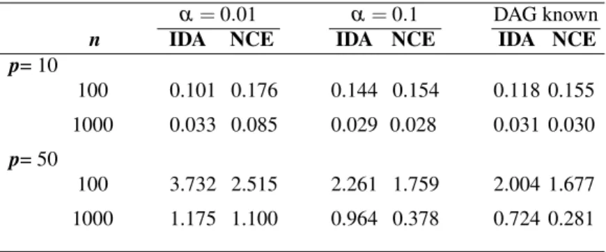
Given that the IDA algorithm is made for these Gaussian data, the method should outperform the NCE method, which is agnostic about the underlying distributional assumptions. We apply the methods to the four data scenarios and the results are presented in the last column of Table 1 as mean absolute deviations. The mean absolute deviation is a robust version of the mean squared error and smaller val-ues refer to better estimates of the causal effects. Table 1 shows that when the number of observations are increasing, the mean absolute deviation for causal ef-fect estimates for both IDA and NCE methods is decreasing. Furthermore, the NCE method, as expected, is somewhat more variable. This variation is mostly the result from the poorer estimates of the distributional shape in the tails of the distribution.

5.1.2 Causal DAG unknown

If the underlying causal DAG is considered unknown, then the CPDAG and asso-ciated DAGs need to be estimated. For each simulation, we run both the standard PC-algorithm and the robust RPC-algorithm on a grid of significance levelsα

rang-ing from 10−10_{to 0.5. For each estimated DAG, we compute the causal effects of}

each node according to the NCE method and the compare the results with the IDA method.

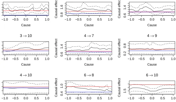
Figures 3 show the causal effects between the chosen nodes for small graph on ten verticesp=10 withn=100. In these figures the red line show the real causal

effect between two chosen nodes. The blue line shows the average estimated causal effect from the IDA method. The black line show the average functional causal ef-fect estimate (7) proposed by our NCE method across the DAGs consistent with the inferred CPDAG. The dashed lines express the average standard deviation of our functional causal effect estimate. A clear message emerges from plots: whereas the IDA method is exactly matched for this simulation scenario, our nonparanor-mal causal effects estimates are quite stable. Moreover, the confidence intervals calculated by our method typically contain the true effect.

In Table 1 provide numerical comparisons of both methods on data sets with different transformations, where we repeat the experiments 100 times and report the mean absolute deviation for causal effect estimates on each pair nodes in both IDA and NCE methods. Even though the simulation method is precisely suited for the IDA method, our NCE method is highly competitive.

5.2 Exponential data

Only in a few special non-Gaussian distributional examples can we calculate the causal effects exactly. This makes large scale simulation studies difficult.

There-−1.0 −0.5 0.0 0.5 1.0 0.6 1.2 1→5 Cause Causal eff ect −1.0 −0.5 0.0 0.5 1.0 0.8 1.6 1→9 Cause Causal eff ect −1.0 −0.5 0.0 0.5 1.0 0.6 1.4 3→7 Cause Causal eff ect −1.0 −0.5 0.0 0.5 1.0 0.5 2.0 3→10 Cause Causal eff ect −1.0 −0.5 0.0 0.5 1.0 0.6 1.4 4→7 Cause Causal eff ect −1.0 −0.5 0.0 0.5 1.0 0.2 0.8 4→9 Cause Causal eff ect −1.0 −0.5 0.0 0.5 1.0 0.0 1.0 4→10 Cause Causal eff ect −1.0 −0.5 0.0 0.5 1.0 0.4 1.0 6→8 Cause Causal eff ect −1.0 −0.5 0.0 0.5 1.0 1.5 6→10 Cause Causal eff ect

Figure 3: Simulation study for Gaussian data from a causal graph (p=10 vertices

withn=100 observations). The red lines are the true (constant) causal effects. The

blue lines are the causal effect estimates from the IDA methods and black lines show the functional causal effect estimates from our NCE method. The dashed lines show the confidence intervals for functional NCE causal effect estimates. fore, in this section we consider the causal effects in a bivariate exponential dis-tribution. We assume only two nodes with exponential marginal distributions and then apply Crane and Hoek (2008) to find the closed form for conditional expec-tation formula for Gaussian copula. We derive the causal effect for the bivariate Gaussian copula. If we have a bivariate Gaussian copula, with dependence param-eterρ, we have E(Y|X=x) = Z R y ∂ ∂yΦ( Φ−1(F(y))−ρΦ−1(G(x)) p 1−ρ2 )dy. (12)

If both marginal distributionsF andGwereN(0,1), the copula would revert back

to the bivariate normal distribution. The Gaussian copula, however, gives us more flexibility, as it can accommodate any type of univariate distributions,F and G.

α=0.01 α=0.1 DAG known

n IDA NCE IDA NCE IDA NCE

p= 10 100 0.101 0.176 0.144 0.154 0.118 0.155 1000 0.033 0.085 0.029 0.028 0.031 0.030 p= 50 100 3.732 2.515 2.261 1.759 2.004 1.677 1000 1.175 1.100 0.964 0.378 0.724 0.281

Table 1: Comparison of mean absolute deviations (smaller is better) for causal effect estimates between our NCE and IDA (Maathuis et al., 2009) methods for small graphs (p=10) and large graphs (p=50) when the data is Gaussian. λx,λy>0. Thus, Equation (12) reduces to

E(Y|X=x) = p 1 1−ρ2 Z R yφ(Φ −1_(1−exp(− λyy))−ρΦ−1(1−exp(−λxx)) p 1−ρ2 ) (13) × λyexp(−λyy) φ(Φ−1(1−exp(−λyy))) dy,

whereφ(x) =Φ0(x)is the standard normal density. Therefore, for a bivariate

non-paranormal with exponential marginals, we obtain the following causal effect, CE(Y|X=x) =− ρ 1−ρ2 Z R yφ 0 (t) λxexp(−λxx) φ(Φ−1(1−exp(−λxx))) × λyexp(−λyy) φ(Φ−1(1−exp(−λyy))) dy (14)

wheret=Φ−1(1−exp(−λyy√))−ρΦ−1(1−exp(−λxx))

1−ρ2 .

In the simulation study we assume that nodeXaffects nodeY, in the following

fashion, X=F−1(Φ(Z1)) Y=F−1 Φ(Z1√+Z2 2 ) ,

whereF is the CDF of an Exponential(1) distribution andZ1,Z2i.i.d.∼ N(0,1). This

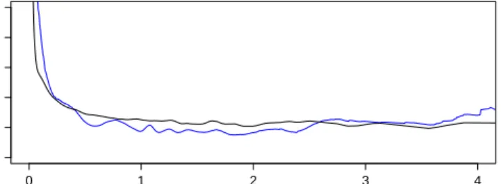
falls under the usual nonparanormal scenario. The explicit expression for the causal effect in Theorem 1 is very involved, but we derived in (14) a simplified expression. We evaluated this expression numerically to obtain the true causal effect, expressed as the solid black line in Figure 4. Then we simulatedn=1,000 observations from

the above model for inferring the causal effect.

We assume that the underlying causal graph,X −→Y, is known and used the

NCE method to infer the non-linear causal effect. The blue line Figure 5.2 shows the functional causal effect estimate from NCE method. It matches very well the true causal effect. Clearly, had IDA been applied in this scenario, it would have come up with a nonsensical constant causal effect.

0 1 2 3 4 0.0 0.2 0.4 0.6 0.8 1.0 Cause Causal Eff ect

Figure 4: Exponential nonparanormal simulation: black line shows the true causal effect and the blue line represents the causal effect estimated by our NCE method.

5.3 Cauchy data

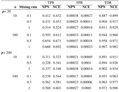
Although not the primary aim of our NCE method, it also consists of the RPC causal graph reconstruction method and can therefore be compared to the NPN method by Teramoto et al. (2014). We evaluated the performance of our NCE and the NPN methods for two different graph sizes: with 20 vertices and 200 vertices. We repeated this experiment 50 times forn∈ {10,100}.

We consider distributional systems whereby the underlying marginal distribu-tions are mixtures of normal and Cauchy distribudistribu-tions. The mixing rate indicates the percentage of samples whose error distribution was drawn from the standard Cauchy distribution. We chose mixing rate 0.1, 0.5 and 1. The higher the mixing rate, the less accurate is the Gaussianity assumption. We averaged the values of true positive rate (TPR), false positive rate (FPR), true discovery rate (TDR) in the reconstruction of the causal graph. To compare NCE method with NPN method,

TPR FPR TDR

n Mixing rate NPN NCE NPN NCE NPN NCE

p= 20 10 0.1 0.412 0.432 0.00038 0.00027 0.887 0.899 0.5 0.431 0.453 0.00025 0.00011 0.904 0.917 1 0.514 0.524 0.00027 0.00016 0.911 0.929 100 0.1 0.593 0.612 0.00033 0.00011 0.944 0.960 0.5 0.654 0.671 0.00037 0.00018 0.958 0.971 1 0.668 0.692 0.00041 0.00023 0.967 0.982 p= 200 10 0.1 0.311 0.323 0.00021 0.00005 0.891 0.911 0.5 0.328 0.341 0.00032 0.0001 0.894 0.928 1 0.337 0.348 0.00038 0.00014 0.902 0.934 100 0.1 0.538 0.544 0.00017 0.00001 0.951 0.963 0.5 0.562 0.581 0.00023 0.00006 0.963 0.977 1 0.588 0.601 0.00027 0.0001 0.971 0.988

Table 2: Mean true positive, false positive and true discovery rates for the compari-son of our NCE and NPN (Teramoto et al., 2014) methods for small graph (p=20)

and large graph (p=200) when the data is Cauchy.

we show the representative results of setting forα=10−4in Table 2. It is clear that

the NCE method, with its underlying RPC causal reconstruction method, always outperforms the NPN method.

6

TiMet: circadian regulation in

Arabidopsis Thaliana

In this section, we illustrate our proposed approach by applying it to a time course gene expression dataset related to the study of circadian regulation in plants. The data used in our study come from the EU project TiMet (FP7-245143, 2014), whose objective is the elucidation of the interaction between circadian regulation and metabolism in plants.

The data consist of transcription profiles for the core clock genes from the leaves of various genetic variants ofArabidopsis Thaliana. The transcription

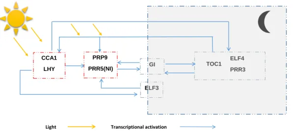
Light Transcriptional activation PRP9 PRR5(NI) ELF3 CCA1 LHY GI ELF4 PRR3 TOC1

Figure 5: The inferred causal network among the circadian clock genes for Ara-bidopsis thaliana. The representation is inspired by Figure 1 in Jia and Huan

(2009), showing significant overlap in topology.

Hodge, Stratford, Knox, Edwards, Thomson, Mizuno, and Millar, 2010, Guerriero, Pokhilko, Fern´andez, Halliday, Millar, and Hillston, 2012) were recorded: LHY, CCA1, PRR3, NI (PRR5), PRR9, TOC1, ELF3, ELF4 and GI. The plants were grown in the following 3 light conditions: a diurnal cycle with 12 hour light and 12 hour darkness (12L/12D), an extended night with full darkness for 24 hours, and an extended light with constant light for 24 hours. An exception is the ELF3 mutant, which was grown only in 12L/12D condition. Samples were taken every 2 hours to measure mRNA concentrations. We consider the same group of nine genes, which from previous studies are known to be involved in circadian reg-ulation (Grzegorczyk and Husmeier, 2011a,b, Grzegorczyk, Husmeier, Edwards, Ghazal, and Millar, 2008, Jia and Huan, 2009). They consist of two groups of genes: “Morning genes”, which are LHY, CCA1, PRR9, and PRR5, whose expres-sion peaks in the morning, and “Evening genes”, including TOC1, ELF4, ELF3, GI, and PRR3, whose expression peaks in the evening. The expressions for all the genes are strictly positive and highly right-skewed.

In traditional analysis of microarray studies, data are typically log-transformed. Especially when using the data for prediction, such transformations are sensible as they typically stabilize variances and make down-stream analyses more robust. In our case, however, our aim is to describe the system. We arenotinterested in the

causal effect of the log-transformed variables, but we are interested in the causal effects of the original variables. For this reason, we consider the raw data directly, since this is the scale on which we would like to evaluate the system.

For inferring the underlying causal CPDAG, we considered the RPC-algorithm in the version that uses the Kendall’s tau — results using Spearman’s rho were almost the same. The CPDAG contains three Markov equivalence DAGs. One of these three causal networks among the genes is displayed in Figure 5. For all three causal DAGs, we infer the causal effects between the genes and these are shown as lines in Figure 6. A striking feature is that most of the causal effects shrink towards zero for large values of the cause, possibly indicating saturation. Moreover, this effect seems stronger for the morning genes on the evening genes than vice versa.

The morning gene CCA1 was found to repress the evening genes EFL3 and NI. Among the evening genes, EFL4 and TOC1 have the strongest effect on both other evening and morning genes. The evening gene ELF positively affects CCA1. It also has a negative effect on LHY. Moreover, the evening genes ELF3, GI and TOC1 are involved in the activation of the morning gene PRR. The morning gene LHY has an almost constant effect on the evening genes ELF4, TOC1 and EFL4. In particular ELF4 interacts positively with NI and CCA1 and negatively with LHY. Many of these results are consistent with the findings in Grzegorczyk and Husmeier (2011a,b), Aderhold et al. (2014) and references therein.

Furthermore, we compare our network with the biological network referred to in Jia and Huan (2009), which is based on the work of Mas (2008) and Salome and McClung (2004). The most striking difference is that we have found evidence that the GI and ELF3 genes interact directly with the Pseudo-Response Regula-tors (PRR9 and PRR5 module). Chow, Helfer, Nusinow, and Kay (2012) suggest that this may be explained by the fact that another protein, LUX, which is not considered in this study, creates a complex with ELF3 that is required to regulate PRR9. This is an interesting methodological issue: studies based on lab-based pairwise interaction studies or studies looking for structural evidence of binding between proteins will not find links between proteins that are not directly interact-ing, whereas studies such as ours that perform network based analysis on a limited number of proteins will typically infer links between proteins that in reality require an intermediary not considered in the study.

7

Conclusion

In this paper, we have derived an explicit formula for causal effects in a flexi-ble class of distributions, the so-called nonparanormal. These distributions are

1.0 1.5 2.0 2.5 −30 −15 0 LHY (morning) C

CA1 (morning) DAG 1

DAG 2 DAG 3 1.0 1.5 2.0 2.5 −20 −10 0 LHY (morning) PRR3 (evening) DAG 1 DAG 2 DAG 3 1.0 1.5 2.0 2.5 0 2 4 6 CCA1 (morning) ELF3 (evening) DAG 1 DAG 2 DAG 3 1.0 1.5 2.0 2.5 −12 −6 ELF4 (evening) LHY (morning) DAG 1 DAG 2 DAG 3 1.0 1.5 2.0 2.5 5 15 ELF4 (evening) C CA1 (morning) DAG 1 DAG 2 DAG 3 1.0 1.5 2.0 2.5 −5 −3 −1 ELF3 (evening) PRR9 (morning) DAG 1 DAG 2 DAG 3 1.0 1.5 2.0 2.5 0 10 20 30 GI (evening) PRR9 (morning) DAG 1 DAG 2 DAG 3 1.0 1.5 2.0 2.5 0 4 8 12 GI (evening) NI (morning) DAG 1 DAG 2 DAG 3 1.0 1.5 2.0 2.5 PRR3 (evening) CCA1 (morning) 0 4 8 DAG 1DAG 2 DAG 3

Figure 6: Causal effects for the circadian gene interaction network inArabidopsis thaliana. Whereas ELF3 and ELF4 have almost constant causal effects, most of

the others have a distinctive shrinkage in their causal effects for larger values of the cause, indicating saturation.

especially useful for real-life observational studies, where normality assumptions are often not warranted. We presented a simple method, NCE, to estimate these causal effects nonparametrically, based on a first order approximation of the gen-eral causal effect formula. It is able to capture a large range of non-linear causal effects and is shown to be consistent under certain conditions. In a simulation study, we have shown that the estimation method works well, particularly away from the tails of the data. We have also applied the method to an Arabidopsis Thalianacircadian clock network. The estimated causal effects reveal a tendency

for some of the causal effects to shrink to zero for large values of the cause, which means that gene regulation shows effect saturation for high levels of the regula-tor. This is in correspondence with simple Michaelis-Menten kinetic models, often used to model gene regulation.

8

Appendix: Proofs

Proof of Theorem 1

Proof. We follow three steps for proving this theorem. First, we find a closed form

expression for EY|Xi=xi;Xpa(i)=xpa(i)

. After that we connect this to the do-operator as is done in (2). Finally, taking the derivative in the way that the total causal effect is defined in (1) will complete the proof. From the differentiability of

fi it follows that the marginal distributions Fi are one-to-one, where fi−1(xi) =zi

andZi= fi−1(Xi) =Φ

−1_{◦Fi(Xi)andZ= f}−1

y (Y) =Φ−1◦Fy(Y). Using the Taylor

expansion, EY|Xi=xi;Xpa(i)=xpa(i) =E(F_y−1(Φ(Z))|Xi=xi;Xpa(i)=xpa(i)) =E(F_y−1(Φ(Z))|Zi=zi;Zpa(i)=zpa(i)) =E(fy(Z)|Zi=zi;Zpa(i)=zpa(i)) =E( ∞

∑

∑

whereZ∗=Z−z₀ for anyz₀∈_R. From the conditional normal distribution,

we know that

Z∗|Zi=zi;Zpa(i)=zpa(i)∼N(−z0+ (βi,βpa(i))(zi,zpa(i))T,(1−ρ2)).

where (βi,βpa(i)) = Σp,(i,pa(i))Σ−₍i,pa1 (i)),(i,pa(i)) and

ρ= Σp,(i,pa(i))Σ−₍i,pa1 (i)),(i,pa(i))Σ(i,pa(i)),p.

Following Lehmann and Casella (1998) page 132, we get fork∈_N E(Z∗k|Zi=zi;Zpa(i)=zpa(i)) = bk 2c

∑

Plugging (16) into (15), we have

E(Y|Xi=xi;Xpa(i)=xpa(i)) = ∞

∑

∑

Now we use (17) for finding the intervention effect for nonparanormal variable. That is, E(Y|_do(Xi=xi)) = Z E(Y|Xi=xi;Xpa(i)=xpa(i))P(xpa(i))d(xpa(i)) = ∞

∑

∑

∑

∑

∑

∑

We get the following expression for the total causal effect,

∂ ∂xi E[Y|do(Xi=xi)] = ∂ ∂zi E[Y|do(Xi=xi)] ∂zi ∂xi , (19) where ∂zi ∂xi = (f −1

i )0(xi). Therefore, with plugging (18) into (19), the proof is

com-pleted. Proof of Proposition 3 Proof. Define ˆ Zn=      ˆ z_1,i zˆ1,pa(i)1 · · · zˆ1,pa(i)k ˆ z2,i zˆ2,pa(i)1 · · · zˆ2,pa(i)k ... ... ... ... ˆ zN,i zˆN,pa(i)1 · · · zˆN,pa(i)k     ,

such that ˆzj,l =Φ−1(Fˆl,n(xjl))wherexjl is the non-ordered jth sample of variable

land pa(i)is the index set ofkparents ofi.Let

ˆ ϒTn = Φ −1_(Fˆ y,n(y1)),Φ−1(Fˆy,n(y2)),· · ·,Φ−1(Fˆy,n(yN)) .

The coefficient ˆβinis defined as the first element of the vector,

ˆ

We can also define the oracle estimator ˆBn_i as the first element of

ˆ

Bn= (Z_ntZn)−1Ztϒn,

whereZnandϒnare obtained by replacing the marginal ˆFs by the trueFs. Consider

an arbitraryε,δ>0, P(|βˆ_in−βi|>ε) =P(|βˆin−Bˆ n i +Bˆ n i −βi|>ε) ≤P((|βˆ_in−Bˆn_i|+|Bˆn_i −βi|)>ε) ≤P((|βˆin−Bˆni|>ε/2) +P(|Bˆni −βi|)>ε/2). (20)

We first consider the first right hand side term of (20). Let’s define ˆAn =

ˆ Zt_nZˆn n , An=Z t nZn n and ˆbn= ˆ Zt nϒnˆ n andbn= Zt nϒn n . Then, P(|βˆin−Bˆ n i|> ε 2)≤P(kAˆ −1 n bˆn−A−n1bnk2> ε 2) ≤P(kAˆ−_n1(bˆn−bn)k2 +k(Aˆ−_n1−A−_n1)bnk2> ε 2) ≤P(kAˆ−_n1(bˆn−bn)k2> ε 4) +P(k(Aˆ−_n1−A−_n1)bnk2> ε 4). (21) By the consistency of ˆz, we have that both ˆbn andbn converge in probability to

someb=Σ(i,pa(i)),pand both ˆA−n1andA−n1converge in probability to someA−1=

Σ−_(i,pa1 _{(i)),(i,pa(i))}, whereΣis defined in the body of Theorem 1. Therefore, there is a

n∗, such that for alln≥n∗, both terms on the right hand side of (21) are less than

δ/4. So for alln≥n∗,

P(|βˆ_in−Bˆn_i|>ε

2)<

δ

2.

For the second term of the right hand side of (20), it is sufficient to use the fact that in the latent normal space a regression estimate is consistent and therefore, there exist an⊥, such that anyn>n⊥,

P(|Bˆn_i −βi|>ε/2)<δ/2.

Putting both results together, we now have that for anyn≥max{n∗,n⊥}, P(|βˆin−βi|>ε)<δ.

Proof of Proposition 4

Proof. For two sequences of random variablesZnandWnand two random variables

Z,W, such thatZnconverges in probability toZandWnconverges in probability to

W, then it is a standard result thatZnWnconverges in probability toZW(Lehmann,

2004). As all the components ofNCEd0(x)have been shown to be consistent, then

the estimator is consistent.

References

Aderhold, A., D. Husmeier, and M. Grzegorczyk (2014): “Statistical inference of regulatory networks for circadian regulation,”Statistical applications in genetics and molecular biology, 13, 227–273.

Anderson, T. (2003): An introduction to multivariate statistical analysis, Wiley

series in probability and statistics,New YorkChichester: Wiley.

Chickering, D. M. (2002): “Learning equivalence classes of bayesian-network structures,”The Journal of Machine Learning Research, 2, 445–498.

Chickering, D. M. (2003): “Optimal structure identification with greedy search,”

The Journal of Machine Learning Research, 3, 507–554.

Chow, B. Y., A. Helfer, D. A. Nusinow, and S. A. Kay (2012): “Elf3 recruitment to the prr9 promoter requires other evening complex members in the arabidopsis circadian clock,”Plant signaling & behavior, 7, 170–173.

Crane, G. J. and J. v. d. Hoek (2008): “Conditional expectation formulae for copu-las,”Australian & New Zealand Journal of Statistics, 50, 53–67.

Grzegorczyk, M. and D. Husmeier (2011a): “Improvements in the reconstruction of time-varying gene regulatory networks: dynamic programming and regular-ization by information sharing among genes,”Bioinformatics, 27, 693–699.

Grzegorczyk, M. and D. Husmeier (2011b): “Non-homogeneous dynamic bayesian networks for continuous data,”Machine Learning, 83, 355–419.

Grzegorczyk, M., D. Husmeier, K. D. Edwards, P. Ghazal, and A. J. Millar (2008): “Modelling non-stationary gene regulatory processes with a non-homogeneous bayesian network and the allocation sampler,”Bioinformatics, 24, 2071–2078.

Guerriero, M. L., A. Pokhilko, A. P. Fern´andez, K. J. Halliday, A. J. Millar, and J. Hillston (2012): “Stochastic properties of the plant circadian clock,”Journal of The Royal Society Interface, 744–756.

Gugushvili, S. and C. A. J. Klaassen (2012): “√n-consistent parameter estimation

for systems of ordinary differential equations: bypassing numerical integration via smoothing,”Bernoulli, 18, 1061–1098.

Harris, N. and M. Drton (2013): “Pc algorithm for nonparanormal graphical mod-els,”The Journal of Machine Learning Research, 14, 3365–3383.

Heckerman, D. and D. Geiger (1995): “Learning bayesian networks: a unification for discrete and gaussian domains,” inProceedings of the Eleventh conference on Uncertainty in artificial intelligence, Morgan Kaufmann Publishers Inc., 274–

284.

Jia, Y. and J. Huan (2009): “The analysis of arabidopsis thaliana circadian network based on non-stationary dbns approach with flexible time lag choosing mecha-nism,” inBioinformatics and Biomedicine, 2009. BIBM’09. IEEE International Conference on, IEEE, 178–181.

Kalisch, M. and P. B¨uhlmann (2007): “Estimating high-dimensional directed acyclic graphs with the pc-algorithm,” The Journal of Machine Learning Re-search, 8, 613–636.

Lehmann, E. L. (2004):Elements of large-sample theory, Springer Science &

Busi-ness Media.

Lehmann, E. L. and G. Casella (1998): Theory of point estimation, volume 31,

Springer Science & Business Media.

Liu, H., F. Han, M. Yuan, J. Lafferty, and L. Wasserman (2012): “High-dimensional semiparametric gaussian copula graphical models,”The Annals of Statistics, 40, 2293–2326.

Maathuis, M. H., M. Kalisch, and P. B¨uhlmann (2009): “Estimating high-dimensional intervention effects from observational data,”The Annals of Statis-tics, 37, 3133–3164.

Mas, P. (2008): “Circadian clock function in arabidopsis thaliana: time beyond transcription,”Trends in cell biology, 18, 273–281.

Mooij, J. M., D. Janzing, T. Heskes, and B. Sch¨olkopf (2011): “On causal dis-covery with cyclic additive noise models,” inAdvances in neural information

Nandy, P., M. H. Maathuis, and T. S. Richardson (2017): “Estimating the effect of joint interventions from observational data in sparse high-dimensional settings,”

The Annals of Statistics, 45, 647–674.

Pearl, J. (1995): “Causal diagrams for empirical research,”Biometrika, 82, 669–

688.

Pearl, J. (2009):Causality, Cambridge university press.

Pokhilko, A., S. K. Hodge, K. Stratford, K. Knox, K. D. Edwards, A. W. Thomson, T. Mizuno, and A. J. Millar (2010): “Data assimilation constrains new connec-tions and components in a complex, eukaryotic circadian clock model,” Molec-ular systems biology, 6, 416.

Priestley, M. and M. Chao (1972): “Non-parametric function fitting,”Journal of the Royal Statistical Society. Series B (Methodological), 385–392.

Richardson, T. (1996): “A discovery algorithm for directed cyclic graphs,” Pro-ceedings of the Twelfth international conference on Uncertainty in artificial in-telligence, 454–461.

Salome, P. A. and C. R. McClung (2004): “The arabidopsis thaliana clock,” Jour-nal of Biological Rhythms, 19, 425–435.

Spiegelhalter, D. J., A. P. Dawid, S. L. Lauritzen, and R. G. Cowell (1993): “Bayesian analysis in expert systems,”Statistical science, 219–247.

Spirtes, P., C. N. Glymour, and R. Scheines (2000): Causation, prediction, and search, volume 81, MIT press.

Spirtes, P., C. Meek, and T. Richardson (1995): “Causal inference in the presence of latent variables and selection bias,” Proceedings of the Eleventh conference on Uncertainty in artificial intelligence, 499–506.

Teramoto, R., C. Saito, and S.-i. Funahashi (2014): “Estimating causal effects with a non-paranormal method for the design of efficient intervention experiments,”

BMC bioinformatics, 15, 228.

Verma, T. and J. Pearl (1990): “Equivalence and synthesis of causal models [tech-nical report r-150],”Department of Computer Science, University of California, Los Angeles.