https://doi.org/10.5194/ms-10-255-2019
© Author(s) 2019. This work is distributed under the Creative Commons Attribution 4.0 License.
Mechanism design and parameter optimization of a new
asymmetric translational parallel manipulator
Yi Yang, Yaqi Tang, Haijun Chen, Yan Peng, and Huayan Pu
School of Mechatronic Engineering and Automation, Shanghai University, Shanghai, 200444, China
Correspondence:Yan Peng (pengyan@shu.edu.cn)
Received: 6 November 2018 – Revised: 18 February 2019 – Accepted: 23 May 2019 – Published: 18 June 2019
Abstract. With the requirement of heavy load for pick-and-place operation, a new 3-DoF asymmetric trans-lational parallel manipulator is invented in this paper. This manipulator is assembled by a kinematic limb with the parallel linear motion elements(PLMEs), and a single loop 2-UPR. Owning to the linear actuators directly connecting the moving and the fixed platforms, this parallel manipulator has high force transmission efficiency, and adapts to pick-and-place operation under heavy load. In this paper, the mobility and singularity are firstly analyzed by screw theory. And the simplified kinematic and dynamic model is established and solved. Secondly, the reaction forces of the prismatic joints in the PLMEs limb are investigated for the mechanism design. Also, the overall performance of the whole manipulator, such as the workspace, condition numbers of Jacobian ma-trices and motion transmission, etc, are discussed. Thirdly, a compound evaluation function, which involves the factors of workspace volume, transmission efficiency and reaction force, is proposed. In order to obtain a set of better design parameters, the optimization of the 3-DoF translational manipulator is conducted, for the object of maximum of the evaluation function. At last, the prototype is manufactured and experimented to validate the mobility and motion feasibility of this mechanism design.
1 Introduction
As the need of the industry for 3-DoF translational parallel mechanisms(TPM) in the late 1990s, many these kinds of parallel mechanisms have been researched and developed. In academic, several approaches for the type synthesis of TPMs were investigated, such as methods based on screw theory (Mohamed et al., 1985; Lee et al., 1999; Zhao et al., 2002; Bonev et al., 2003; Huang and Li, 2003; Kong and Gos-selin, 2004a; Dai, 2006, 2014; Dai et al., 2006; Wu et al., 2010; Zhao et al., 2017), displacement group theory (Hervé, 1999; Lee et al., 2009), position and orientation characteris-tic (POC) sets (Yang et al., 2009), generalized function (GF) sets (Gao et al., 2011) and etc. By these means, a number of novel TPMs were invented by Tsai and Joshi (2000); Chab-lat and Wenger (2003); Liu et al. (2003); Kong and Gos-selin (2004b); Jin and Yang (2004); Gogu (2008); Yang et al. (2019) and et al. And the kinematics, dynamics, singularities, stiffness, workspaces for the 3-DOF TPMs were contributed by Carricato and Parenti-Castelli (2002); Li and Xu (2008);
Liu et al. (2017); Kong and Gosselin (2002); Li et al. (2015); Zhang et al. (2017), amongst others.
The actuators among the above TPMs can be divided into 2 primitive types, i.e, rotational actuators and linear actuators. The well-known 3-DoF TPM, Delta robot, is driven by 3 ro-tational actuators located on the base (Pierrot et al., 1990). Due to its capacity of high speed and high accelerations, this robot has popular usage in picking and packaging in facto-ries. In 1996, Tsai proposed a typical 3-UPU parallel robot, called Tsai manipulator (Tsai and Joshi, 2000). The prismatic joint in each leg is driven by one linear actuator. Compared with the rotational actuators, the linear actuators generally deliver large force at high efficiency due to the simple trans-mission structure, and are used in a wide range of application in industry, especially in heavy duty equipments. Therefore, in the design of the heavy-load translational parallel manip-ulator, we choose the linear actuators to drive the moving platform of TPM in this paper.
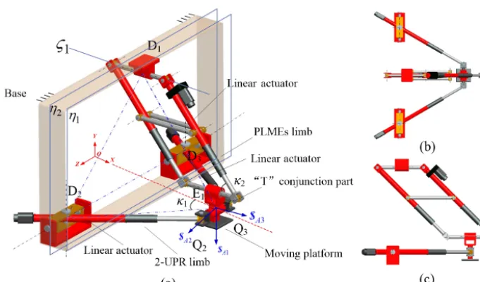
Figure 1.A 3-DoF translational manipulator with PLMEs limb and single loop 2-UPR:(a)oblique view,(b)top view,(c)side view.
(2002) showed that the small torsions in the legs of 3-UPU generated large deviations in the position of the moving platform. Thus, the applications of the Tsai’s manipulator are limited in industry. The “Linear Deltas” has been de-veloped from the standard Delta robot (Bouri and Clavel, 2010). The linear actuators move the parallelograms in each leg up or down, and then lead to the translating of the end platform. Furthermore, Yang et al. (2018) proposed a novel kind of kinematic chains with parallel linear motion elements(PLMEs), and synthesized a class of symmetrical 3T, 3T-1R, and 3R parallel mechanisms by these kinematic limbs. Different from “Linear Delta”, the linear actuators in these limbs directly connect the moving platform and the fixed base, which makes the parallel manipulators capable of higher transmission efficiency. Inspired by the above schol-ars’ achievements, we propose a new 3-DoF translational manipulator by combining of PLMEs limb and single loop 2-UPR (Peng et al., 2018). This kind of manipulator has advan-tage of better transmission and simpler structure than other 3-DoF TPMs.
The rest of the paper is organized as follows. In Sect. 2, the structure is elaborated, and the mobility and singularity are analyzed. In Sect. 3, the kinematic and dynamic model is established and solved. In Sect. 4, the reaction forces of the prismatic joints in the PLMEs limb are studied. In Sect. 5, the overall performance of the whole manipulator, such as the workspace, condition numbers of Jacobian matrices and mo-tion transmission, etc, are evaluated. In Sect. 6, a compound evaluation function is proposed. And the parameters of this manipulator are optimized. Finally, in Sect. 7, the prototypes are manufactured and validate the mobility and motion fea-sibility of this new manipulator.
2 Structure and mobility of the new manipulator
The new 3-DoF manipulator is assembled by the parallel lin-ear motion elements(PLMEs) limb and a single loop 2-UPR, as shown in Fig. 1. The moving platform is driven by 3 lin-ear actuators, i.e., one actuator located in PLMEs limb and the other two actuators located in the single loop 2-UPR. To investigate the mobility and singularity of this new manipu-lator, we firstly analyze the PLMEs limb and the 2-UPR limb individually, by the utilization of screw theory. Secondly, we express the screws of the mechanism by Grassmann line ge-ometry, and obtain the DoF space of the whole manipulator. Furthermore, we also discuss the controllability of the mov-ing platform driven by the 3 selected linear actuators.
As an effective tool, screw theory is widely applied to an-alyze the mobility, singularity, transmission of mechanisms. A screw is usually represented by the form of Plucker ho-mogeneous coordinates (L,M,N,P,Q,R). In mechanism research, the general term “screw” can be divided into twist $and wrench$r. In twist$, the first three components denote an instantaneous angular velocity around an axis. And the last three components denote an instantaneous linear veloc-ity along this axis. In wrench$r, The first three components denote the resultant force and the last three components de-note the resultant moment. If the reciprocal product of the two screws,$and$r, equals zero, these two screws are said to be reciprocal. The details can be found in Kong and Gos-selin (2004a); Dai et al. (2006); Dai (2014), etc.
2.1 PLMEs limb
Figure 2.PLMEs limb.
tubes are able to slide along axesA1B1andA2B2, respec-tively.
With reference (Yang et al., 2018), the moving linkC1C2 generally has 2 translational DoFs without consideration of the revolute joints D1 and E1. The PLMEs linkage
A1A2C1C2can be regarded as a generalized kinematic pair, whose twist is denoted as {$g1,$g2}. Adding the revolute jointsD1 andE1, the twist of the platformP1 is then writ-ten as in Eq. (1) if the PLMEs linkage is not in a singular configuration.
$p1:=
$D1= 1 0 0 0 0 −yd1 $g1= 0 0 0 cosθ1 sinθ1 0 $g2= 0 0 0 −l1sinθ1 l1cosθ1 0 $E1= 1 0 0 0 0 −ye1
(1)
Its corresponding reciprocal screw$rspcan be obtained as
$rp1:= (
$r1sp1= 0 0 0 0 0 1
$r2sp1= 0 0 0 0 1 0 (2)
Equation (2) can be represented by the constraint space graph as shown in Fig. 5a. Whenθ1= ±π/2 , this configuration is a singularity. The Z axis rotational constraint is absent and the constraints reduce to only one. The kinematic limb has an extra instantaneous rotation aboutZaxis. Considering the rotating of this limb alongXaxis, this kind of singular con-figurations are all distributed on the planeη1 , as shown in Fig. 2. When θ1=0, π, the axes of the revolute joints D1 andE1 are collinear and the twists$D1and$E1 are corre-lation. In this case, the moving platform has an additional instantaneous constraint to prevent it from translating along
Zaxis.This singular configuration is on the lineς1, as shown in Fig. 2.
In the above PLMEs limb, the mid-link B1B2 connects the 2 outer tubes of the linear motion elements, as shown in Fig. 3a. In actual design, we can change the mid-linkB1B2 from the outer tubes to the inner tubes, as shown in Fig. 3b. The parallelogramB1C1B2C2guaranteesA1C1andA2C2be
always parallel. Thus, the mobility, constraint and singular-ity are as the same as the one in Fig. 3a. In another case, as shown in Fig. 3c, the mid-linkB1B2is fixed on the ground. The two sliders on the pointsB1andB2are jointed with the mid-link. The two linear guidesA1C1 andA2C2 can slide onB1andB2. The linkageA1C1A2C2is a parallelogram. Therefore, the PLMEs presented in Fig. 3c has also the same kinematic characteristics with the above two ones. From the kinematic point of view, these three PLMEs limbs presented in Fig. 3 are all equivalent.
2.2 Single Loop 2-UPR
This single loop is constructed by 2 UPR limbs, as illustrated in Fig. 4. In Limb D2Q2 , one axis of the universal joint
D2is perpendicular withX–Y plane. The axis orientation is
s1=(0,0,1) . The other axis is perpendicular with the plane formed by the vectorss1and pQ2−pD2
, wherepQ
2 and
pD
2 are the coordinates of the pointsQ2andD2. This axis orientation can be written ass2=s1×(pQ2−pD2). The axis of another jointQ2is parallel with the vectors2. The other LimbD3Q3has the similar condition withD2Q2.
For LimbD2Q2, the twist of each kinematic pair can be written as
$11= s1; pD2×s1 $12= s2; pD2×s2 $13= 0; pQ
2−pD2
$14= s2; pQ2×s2
(3)
Through calculating the nullity of the above screws, the cor-responding reciprocal screw of limbD2Q2can be obtained as
$rQ
2:= (4)
$r1Q
2=
0, 0, 0, (xa1−xc1), (ya1−yc1), 0
$r2Q 2=
−(ya1−yc1), (xa1−xc1), 0, 0, 0,
xa1(xa1−xc1)+ya1(ya1−yc1)
In the same way, the wrench of limbD3Q3is
$rQ
3:= (5)
$r1Q
3=
0, 0, 0, (xa2−xc2), (ya2−yc2), 0
$r2Q 3=
−(ya2−yc2), (xa2−xc2), 0, 0, 0,
xa2(xa2−xc2)+ya2(ya2−yc2)
If Q2Q3 andD2D3 are parallel with each other and both perpendicular withX–Y plane, the coordinates of the joints satisfy
xa2=xa1, ya2=ya1, xc2=xc1, yc2=yc1 (6)
Figure 3.Three equivalent PLMEs limbs:(a)mid-link connecting outer tubes,(b)mid-link connecting inner tubes,(c)mid-link fixing on the ground.
Figure 4.Single Loop 2-UPR.
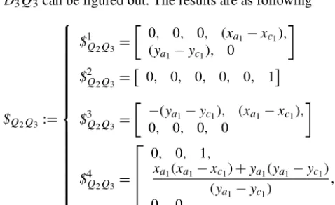
D3Q3can be figured out. The results are as following
$Q2Q3 :=
$1Q 2Q3=
0, 0, 0, (xa1−xc1), (ya1−yc1), 0
$2Q 2Q3=
0, 0, 0, 0, 0, 1
$3Q 2Q3=
−(ya1−yc1), (xa1−xc1), 0, 0, 0, 0
$4Q 2Q3=
0, 0, 1,
xa1(xa1−xc1)+ya1(ya1−yc1) (ya1−yc1)
,
0, 0
(7) Within the consideration of the revolute pairE2attached on the linkQ2Q3, the twist of the platformP2can then be ex-pressed as
$p2:=
$Q2Q3 $E2=
0, 0, 1, ye2, −xe2, 0
(8)
By solving the nullity of Eq. (8), the wrench of the moving platformP2can be obtained.
$rp 2=
0 0 0 xa1−xc1 ya1−yc1 0
(9) According to Eq. (9), the corresponding constraint space graph of the moving platform P2 is plotted as shown in Fig. 5b. Moreover, we substituteS-joint forU-joint. The sin-gle loop 2-SPR is instead of the loop 2-UPR. By repeating the above analysis process, it can be derived that the wrench of the moving platformP2in this case still equals Eq. (9). This means that the loops 2-UPR and 2-SPR are equivalent and they can be swapped with each other for the requirements.
2.3 Whole manipulator
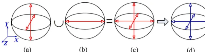
Figure 5.Constraint and DoF space graph of the whole manipulator:(a)PLMEs limb,(b)Single Loop 2-UPR,(c)Constraint space of moving platform,(d)DoF space of moving platform.
used in the research on mechanism, especially on the DoFs and constraints of a mechanism. The line graph can be used to express an n-dimensional DoF space or constraint space in a mechanism. Blanding proposed a basic rule to uncover this dual relationship and mutual converse of the DoF spaces and constraint spaces through line graph. The basic rule was summarized by Blanding (1999); Yu et al. (2011), and etc. In this paper, we firstly plot the constraint space of the PLMEs limb and the single loop 2-UPR in one graph with Grassmann line geometry, as shown in Fig. 5c. Secondly, we apply the mutual conversion rule of DoF spaces and constraint spaces (Xie et al., 2013) for Fig. 5c. Then, the DoF space can be quickly obtained as shown in Fig. 5d. The result illustrates that the platform has 3 translational DoFs.
The manipulator has 2 kinds of singularities. One kind of singularity comes from the PLMEs limb. Whenθ1= ±π/2 orθ1=0, π, the PLMEs limb is located on singular Planeη1 or Lineς1, as shown in Fig. 1. In this case, the constraints of the PLMEs limb are instantaneously changed. It results into the varying of the mobility of the manipulator. Another kind of singularity is that the 2-UPR limb are vertical, located on Planeη2. In this case, the constraints of the PLMEs limb and 2-URP limbs are all on Y–Z plane. TheX axis rotational constraint is absent. The moving platform exists an extra in-stantaneous rotation aboutXaxis.
In this manipulator, each limb is assumed to be driven by one linear actuator. Herein, we discuss whether the moving platform can be controlled by these 3 selected linear actua-tors. For the convenience of calculation, the moving platform is regarded as a link, without consideration of the actual geo-metric feature. Thus, the coordinates of the joints in the mov-ing platform yield
xe2=xc2=xc1, ye2=yc2=yc1 (10)
In analysis, the two prismatic joints in the single loop 2-UPR are firstly fixed. The prismatic joint in PLMEs limb is free. In this case, the twist$A1of the moving platform can be obtained as
$A1 =
0, 0, 0, −(ya1−yc1), (xa1−xc1), 0
(11)
Equation (11) illustrates that the moving platform has only one translational mobility under the above condition. The
in-stantaneous velocity is perpendicular with the plane formed byD2Q2andD3Q3.
Secondly, the prismatic joints in PLMEs and LimbD3Q3 are fixed and the prismatic joint in LimbD2Q2 is set to be free. The twist$A2 of the moving platform can be calculated as
$A2 =
0, 0, 0, (za2−zc2) sinθ1, −(za2−zc2) cosθ1,
(ya2−yc2) cosθ1−(xa2−xc2) sinθ1
(12)
Equation (12) illustrates that the moving platform has one translational mobility, which is perpendicular with the plane formed byD1E1andD3Q3.
In the same way, the prismatic joints in PLMEs and Limb
D2Q2are fixed and the prismatic joint in LimbD3Q3is set to be free. The twist$A3 of the moving platform is
$A3 =
0, 0, 0, (za1−zc1) sinθ1, −(za1−zc1) cosθ1,
(ya1−yc1) cosθ1−(xa1−xc1) sinθ1
(13)
Equation (13) illustrates that the only one translational mo-bility is perpendicular with the plane formed byD1E1 and
D2Q2.
According to the above analysis, it can be summarized that the manipulator assembled by PLMEs and 2-UPR limbs gen-erally has 3 pure translational DoFs. And the moving plat-form is controllable by 3 linear actuators.
3 Simplified kinematic and dynamic model
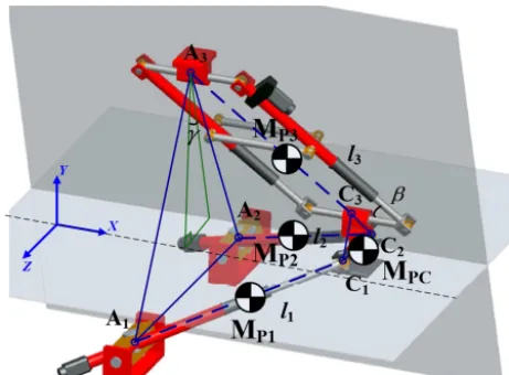
According to the motion characteristics of this manipulator, the 3-DoF translational manipulator can be simplified as a 3-SPS mechanism without rotation mobilities. As shown in Fig. 6, (xC1, yC1, zC1), (xC2, yC2, zC2) and (xC3, yC3, zC3) are the initial positions of the pointsC1,C2andC3of the mov-ing platform. (xA1, yA1, zA1), (xA2, yA2, zA2), (xA3, yA3, zA3) are the initial positions of the pointsA1,A2andA3of the fixed platform, respectively.l1,l2andl3 are the lengths of
Figure 6.Simplified 3-SPS mechanism.
3.1 Displacement equation
Let x, y, z be the displacements of the moving platform
C1C2C3 from the initial position. The displacement equa-tions can be derived as
p
(xC1+x−xA1)2+(yC1+y−yA1)2+(zC1+z−zA1)2=l1
p
(xC2+x−xA2)2+(yC2+y−yA2)2+(zC2+z−zA2)2=l2
p
(xC3+x−xA3)2+(yC3+y−yA3)2+(zC3+z−zA3)2=l3
(14) If the displacement (x, y, z) is known, the driving displace-ments of the linear actuators l1,l2andl3can be easily ob-tained by Eq. (14). Conversely, if the driving displacements
l1,l2andl3are known, the forward displacement of the mov-ing platform (x, y, z) can be found by solving the above 3 equations. Let
XA1=xA1−xC1, XA2=xA2−xC2, XA3=xA3−xC3,
YA1=yA1−yC1, YA2=yA2−yC2, YA3=yA3−yC3,
ZA1=zA1−zC1, ZA2 =zA2−zC2, ZA3=zA3−zC3
and
E11=2 XA2−XA1
, E12=2 YA2−YA1
,
E13=2 ZA2−ZA1
, E31=2 XA3−XA2
,
E32=2 YA3−YA2
, E33=2 ZA3−ZA2
H1=l12−l22+
XA2
2−X 2 A1
+YA2
2−Y 2 A1
+Z2A
2−Z 2 A1
H3=l22−l32+
XA2
3−X 2 A2
+YA2
3−Y 2 A2
+Z2A
3−Z 2 A2
Squaring both sides of Eq. (14), and subtracting the first formula to the second one, and the second one to the third one, Eq. (14) is transformed to
E11x+E12y+E13z=H1
E31x+E32y+E33z=H3
(15)
In this paper, the limbsA1A2andC1C2 are always per-pendicular withX–Y plane. The length projections ofA1C1 andA2C2onX-Y plane are equal. It yields
E11=E12=0 (16)
Through Eqs. (15) and (16), the displacement z can be quickly solved
z=H1/E13 (17)
Then, substituting Eq. (17) into Eqs. (14) and (15), and let
m= −E32/E31, n=(H3−E33H1/E13)/E31,
Pa=m2+1, Pb=2(m(n−XA3)−YA3),
Pc=(n−XA3) 2+Y
A3
2+(z−Z A3)
2−l2 3 The displacementsyandx can be solved by
y=−Pb−
p
Pb2−4PaPc 2Pa
x=my+n
(18)
Equation (17) and (18) give the analytic solution of the for-ward kinematics of the manipulator. Further, we can calcu-late the angleβ (as shown in Fig. 6) in the PLMEs limb by the following formula.
cosβ= (19)
− xC1+x−xA1
p
(xC1+x−xA1)2+(yC1+y−yA1)2+(zC1+z−zA1)2 And the angleγbetween the PLMEs and the horizontal plane (as shown in Fig. 6) is calculated as
tanγ= zC1+z−zA1
yC1+y−yA1
(20)
3.2 Velocity equation
Differentiating Eq. (14) leads to the velocity equation.
Jv ˙ x ˙ y ˙ z = ˙ l1 ˙ l2 ˙ l3 (21)
where the Jacobian matrixJvis
Jv= (22)
(x−xA1+xC1)
l1
(y−yA1+yC1)
l1
(z−zA1+zC1)
l1 (x−xA2+xC2)
l2
(y−yA2+yC2)
l2
(z−zA2+zC2)
l2 (x−xA3+xC3)
l3
(y−yA3+yC3)
l3
(z−zA3+zC3)
l3
y, andzaxes. The absolute value of the determinant of the third-order matrixJvequals the volume of the parallelepiped spanned by each row vector of Jv. If the 3 SPS limbs are collinear or coplanar, the determinant of the Jacobian ma-trix equals zero. This mechanism is in singular configuration, which should be avoided in the motion planning. If an exter-nal force (Fx, Fy, Fz) was exerted on the moving platform, the static driving forces of the linear actuators (f1, f2, f3) corresponding to limbs 1, 2 and 3 could be obtained through the Jacobian matrix.
Fx Fy Fz
=JTv f1 f2 f3 (23)
3.3 Dynamic equation
In the manipulator, the moving platform is assumed to carry a heavy load. Taking the mass of 3 limbs asMP1,MP2 and
MP3, each limb of the manipulator is simplified into a mass point for convenient calculation, which is located in the cen-ter of the limb as shown in Fig. 6. MPC is the mass of the moving platform with the heavy load. Based on these as-sumptions, the simplified dynamics equation can be written as f1 f2 f3
= (24)
JTv−1−MPCI3×3 ¨ x ¨ y ¨ z − 1 2 3 X
i=1
MPiI3×3
¨ x ¨ y ¨ z
+MPCI3×3 gx gy gz + 1 2 3 X
i=1
MPiI3×3
gx gy gz + Fx Fy Fz
whereI3×3is the 3×3 identity matrix.Fx,FyandFzare the external force exerted on the moving platform.gx,gyandgz are the gravitational acceleration. Andfi (i=1,2,3) are the driving forces of the 3 linear actuators. Let
MP =MPCI3×3+ 1 2
3 X
i=1
MPiI3×3 (25)
Assumel˙iandl¨i (i=1,2,3) be the velocity and acceleration of the actuators. Differentiating Eq. (21) and substituting the result into Eq. (24), it leads to
f1 f2 f3
= (26)
−JTv
−1 MPJ−v1
¨ l1 ¨ l2 ¨ l3
− JTv −1
MPJ˙−v1
˙ l1 ˙ l2 ˙ l3
+JTv
−1 MP " gx gy gz #
+JTv−1
Fx Fy Fz ! Considering ˙
J−v1= −Jv−1J˙vJ−v1 (27) and substituting the above equation into Eq. (26), the equa-tion can be rewritten as
f1 f2 f3
= (28)
−JTv−1 MPJ−v1
¨ l1 ¨ l2 ¨ l3
+ JTv −1
MPJ−v1J˙vJ−v1
˙ l1 ˙ l2 ˙ l3
+JTv−1 MP
gx gy gz
!
+ JTv−1 Fx
Fy Fz
!
where the derivative of Jacobian matrixJ˙vis
˙ Jv=
˙
xl1−
∂l1 ∂xx˙+
∂l1 ∂yy˙+
∂l1 ∂zz˙
x−XA1
l12
˙
xl2−
∂l2 ∂xx˙+
∂l2 ∂yy˙+
∂l2 ∂zz˙
x−XA2
l22
˙
xl3−
∂l3 ∂xx˙+
∂l3 ∂yy˙+
∂l3 ∂zz˙
x−XA3
l32
(29)
˙
yl1−
∂l1 ∂xx˙+
∂l1 ∂yy˙+
∂l1 ∂zz˙
y−YA1
l21
˙
yl2−
∂l2 ∂xx˙+
∂l2 ∂yy˙+
∂l2 ∂zz˙
y−YA2
l22
˙
yl3−
∂l3 ∂xx˙+
∂l3 ∂yy˙+
∂l3 ∂zz˙
y−YA3
l23
˙
zl1−
∂l1 ∂xx˙+
∂l1 ∂yy˙+
∂l1 ∂zz˙
z−ZA1
l21
˙
zl2−
∂l2 ∂xx˙+
∂l2 ∂yy˙+
∂l2 ∂zz˙
z−ZA2
l22
˙
zl3− ∂l
3 ∂xx˙+
∂l3 ∂yy˙+
∂l3 ∂zz˙
z−ZA3
l23
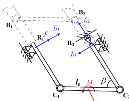
Figure 7. Reaction forces of the prismatic joints in the planar PLMEs limb
Eq. (28) provides a simplified dynamic model for this translational parallel manipulator. It could be used into the control strategy, especially in the high speed pick-and-place operation.
4 Reaction forces of the prismatic joints in the PLMEs limb
In this manipulator, the PLMEs limb provides 2 rotational constraints to the moving platform. The varying of the re-action forces of the two prismatic joints in the PLMEs limb could reveal the performance of the manipulator, i.e., singu-larity, stiffness, etc. Thus, we mainly concern the reaction forces of the prismatic joints in the PLMEs limb in this sec-tion. We firstly study the reaction forces of the prismatic joints in theX–Y plane. Secondly, an external force is ex-erted on the moving platform. And then the reaction forces of the prismatic joints are investigated in the context of the whole manipulator. The results provide the basis for the de-sign of the PLMEs limb in this new translational parallel ma-nipulator.
4.1 Reaction forces in the planar PLMEs limb
In the beginning, we only take the PLMEs limb into the anal-ysis in theX–Y plane, without consideration of the Loop 2-UPR. As shown in Fig. 7,B1C1andB2C2are parallel.R1 andR2are the two prismatic joints. Assumed the actuator is located onR2,B2C2can be regarded to fix on the ground. An external forceF and an external torqueMare exerted on the middle of LinkC1C2, as shown in Fig. 7. The length of Link
C1C2is le. The orientation ofF is along with the PLMEs limb.
Takingfvas the reaction force corresponding to the force
F, andfM as the reaction force corresponding to the torque
M, the following equations are established by means of the
virtual work principle.
F·δ
l e 2cosβ
= −fv·δ(lesinβ)
fM·δ(lesinβ)=M·δβ
(30)
Solving Eq. (30), we can obtain
fv=
F
2 tanβ
fM=
M lecosβ
(31)
By the sum offvandfM, the total reaction forcefR1of the prismatic jointR1can be calculated as the following equa-tion. The orientation offR1 is perpendicular with the pris-matic joint.
fR1=fv+fM =
F
2 tanβ+
M lecosβ
(32)
The reaction forcefR2 of the other prismatic jointR2is decomposed into 2 directions. One direction forcefs1 is per-pendicular with LineB2C2 and opposite to fR1. The other direction forcefs2 is along with LineB2C2and opposite to the actuator forceF. Hence, the component forcesfs1 and
fs2 are written as
fs1= −fR1
fs2= −F
(33)
Observing Eqs. (32) and (33), it is noticed thatfR1 and
fs1 becomes infinite ifβ=π/2. It indicates that the PLMEs limb withβ=π/2 is in the singular configuration, which is consistent with the result derived in Sect. 2.
4.2 Reaction forces in the context of the whole manipulator
Based on the above results, we furthermore investigate the re-action forces of the PLMEs limb in the context of the whole manipulator. The moving platform bears a vertical forceFG as shown in Fig. 8a. Through Eq. (23), the 3 linear actuator forces, denoted as FA1, FA2 andFA3, could be firstly cal-culated out. Secondly, by the utilization ofFA3 and the first row of Eq. (31), one component reaction forcefG1 of the prismatic joints, which is directly corresponding to the force
FA3, can be obtained as following.
fG1=
FA3
2 tanβ (34)
Figure 8.Reaction forces of the prismatic joints in the context of the whole manipulator:(a)side view,(b)front view.
on the “T” conjunction part. The torqueMhcan be obtained by
Mh=fh·e (35)
wherefh is the resultant force ofFA1 andFA2 projected on
Xaxis. As shown in Fig. 8b,Mhcan be decomposed intoM1 andM2by Eq. (36).
M1=Mhcosγ , M2=Mhsinγ (36)
whereM1 andM2 represent the torques be in and perpen-dicular to the plane of PLMEs, respectively. The angleγ be-tween the PLMEs and the horizontal plane can be found by Eq. (20). According to the second row of Eq. (31), the reac-tion forcefG2 corresponding to the torqueM1can be written as
fG2=
M1
lecosβ
(37)
Thus, the total reaction forcefN perpendicular to the pris-matic joint in the plane of PLMEs can be obtained by sum-mingfG1 andfG2.
fN=fG1+fG2=
FA3 2 tanβ+
M1
lecosβ
(38)
In another way, the torqueM2would cause the other reac-tion forcefW perpendicular to the plane of PLMEs. It can be figured out by Eq. (39).
fW =
M2
le
(39)
Finally, through fN andfW, the resultant reaction forcefc of the prismatic joint can be obtained as follows
fc= q
fN2+fW2 (40)
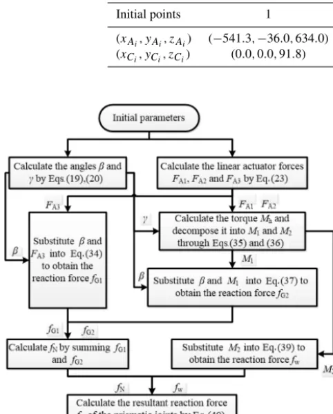
All the above calculation procedure for the force of PLMEs limb is summarized in Fig. 9. It shows that the re-sultant reaction force of the prismatic joints is related to the Jacobian matrix of the manipulator and the configuration of the PLMEs limb. If the reaction force becomes large, it indi-cates the manipulator is in bad performance(e.g., in case of singularity), and vice versa. Through analyzing the force of the prismatic joints in the PLMEs limb, the performance of the manipulator can be revealed.
Based on the above-mentioned results, it is also found that the way of making the external loadFGbe closed to the ac-tuator of PLMEs limb, or decreasing the distanceebetween PLMEs limb and 2-UPR limb could reduce the resultant re-action force of the prismatic joints. It is very helpful for the design of this new translational parallel manipulator.
5 Performance investigation
Based on the aforementioned analysis, we discuss the workspace, condition numbers of Jacobian matrices, simpli-fied dynamics and motion transmission of the new manipula-tor. And the reaction forces of the manipulator under the cir-cumstance that the moving platform bearing a vertical force is also investigated.
5.1 Workspace and Jacobian matrices
Table 1.Coordinates of the initial pointsCi (i=1,2,3) andAi(i=1,2,3).
Initial points 1 2 3
(xAi, yAi, zAi) (−541.3,−36.0,634.0) (−541.3,−36.0,−634.0) (−429.5,441.0,0.0) (xCi, yCi, zCi) (0.0,0.0,91.8) (0.0,0.0,−91.8) (0.0,79.2,0.0)
Figure 9.Calculation procedure for the reaction forces of the pris-matic joints.
Considering the initial configuration, the absolute mo-tion range [lmin, lmax] of each limb is [467.0,1067.0], [467.0,1067.0] and [351.6,771.6], respectively. According to Eq. (14), the workspace of the moving platform is the in-tersection of the 3 hollow spheres, whose inner and outer radii are lmin and lmax. And the centers of the 3 spheres are respectively at (XA1, YA1, ZA1), (XA2, YA2, ZA2) and (XA3, YA3, ZA3). To avoid singularity and consider the ac-tual usage, we just calculate the workspace in the range of y≤441.0 and x≥ −429.5, as shown in Fig. 10a. The workspace of the moving platform is plotted as shown in Fig. 10b–d. The volume of the workspace is calculated to be 1.9755×108mm3.
Furthermore, the condition numbers of Jacobian matri-ces in the workspace is figured out to evaluate the kine-matic performance of the manipulator. In Fig. 11, the condition numbers are plotted as the contour lines on the different layers which are respectively located on the planes y= −400,−300,−200,−100,0,100,200,300 and the plane z=0. The contour lines show that the condition numbers are large when the manipulator approaches the sin-gular configurations, i.e., β=0 and β=π/2. It illustrates that the kinematic property becomes bad when the moving
platform is in these areas. In the proceeding of the motion planning, it is better to avoid these areas.
5.2 Simplified dynamics
In the dynamic analysis, the joint positions of the initial con-figuration are as the same as listed in Table 1. The mass of Limbs 1, 2 and 3 are 2.676, 2.676 and 5.35 kg, respec-tively. And the mass of the moving platform with the load is 11.237 kg. An external forceFy= −100 N is exerted on the moving platform. The gravity is along the negativeY axis. We give the displacement equation dliof each linear actuator relative to the initial configuration as follows.
dli =140 sin π
4t+ 2i
3π
i=1,2,3 (41)
Adding the initial length of each limbloi, the absolute
dis-placement equation of each limb is obtained as
li=loi+ dli i=1,2,3 (42)
Substituting the above conditions into Eq. (28), the actuating force of each limb can be calculated out. To validate the ef-fectiveness of the simplified model deduced in Sect. 3.3, the complete dynamic model is built and simulated in ADAMS software. Two results are presented in Fig. 12, where the solid lines represent the ones come from the simplified dy-namic model, the dashed lines represent the ones come from ADAMS software. It shows that the two curves are generally consistent with each other, although some local errors are a bit of large. The errors come from the simplification of each limb into the mass point. It results in the decreasing of the model accuracy. Nevertheless, the simplified dynamic model still make sense to estimate the actuating force or make con-trol strategy in the design of this manipulator.
Furthermore, the reaction forces of the prismatic joints are also calculated based on the method proposed in Sect. 4.2. The results are compared with the ones obtained by ADAMS software, as shown in Fig. 13. It is found that the two results are similar, which proves the correctness of the method pro-posed in Sect. 4.2.
5.3 Motion transmission
Figure 10.Workspace of the moving platform:(a)oblique view,(b)front view,(c)top view,(d)side view.
Figure 11.Condition numbers of the Jacobian matrices
screw(TWS), denoted $Ti(i=1,2,3), is defined as a unit
screw that are reciprocal to all the twist screws except the ac-tuated one in Limbi. The output twist screw(OTS), denoted $Oi(i=1,2,3), is the instantaneous movement of the
mov-ing platform when fixmov-ing all of its inputs except the one of the
ith limb. The input twist screw(ITS), denoted$li(i=1,2,3),
is the unit twist of the actuated joint in Limbi. And then, for
the given configuration, the input transmission index (ITI) of each limb can be represented as
λi= $Ti◦$Ii
$Ti◦$Ii
max
(i=1,2,3) (43)
trans-Figure 12.Actuating force of each limb:(a)Actuator 1,(b)Actuator 2,(c)Actuator 3.
Figure 13.Reaction forces of the prismatic joints:(a)fN,(b)fW,(c)fC.
mission index of the limb is constant and its value is always equal to 1. It means that this manipulator has high quality of input transmission.
Meanwhile, the output transmission index(OTI) of each limb can be represented as
νi= $Ti◦$Oi
$Ti◦$Oi
max
(i=1,2,3) (44)
The output transmission indexνirepresents the cosine of the angle between the prismatic actuator of Limb iand the in-stantaneous movement of the moving platform. Considering ITI be always equal to 1 in this manipulator, we take the min-imum value ofνias the local transmission index (LTI) of the whole manipulator at the given configuration, denoted asνm. Within the whole workspace, OTIs of each limb of this ma-nipulator can be calculated by Eq. (44). The results are pre-sented as shown in Fig. 14a–c. And the LTIs of the whole manipulator in the workspace are as shown in Fig. 14d. It is found that LTIs in the center of the workspace are gener-ally larger than the ones of the other areas. It illustrates that there is higher efficiency of the motion transmission when the moving platform works in this area.
The above LTIs prescribe the quality of input and out-put transmission in a given configuration. To further evalu-ate the transmissibility of the manipulator within the whole workspace, a global transmission index(GTI) of this manip-ulator is defined as
GTI= R
νmd R
d (45)
whereis the workspace. For this manipulator, GTI over the whole workspace is 0.5664. For the purpose of mak-ing the movmak-ing platform work in the area of better trans-missibility (GTI≥0.7), we search for the maximum area0
in the workspace where GTI≥0.7, termed as the efficient workspace.
Find:0⊂
min: |GTI−0.7| (46)
Through Genetic Algorithm (GA), the efficient workspace0
can be obtained as shown in Fig. 15. The volume of the area
0is 8.26×107mm3, about 41.8 % of the whole workspace.
5.4 Reaction forces of the prismatic joints
A vertical force FG= [0,−100,0] is exerted on the mov-ing platform. By Eq. (23), the forces of the actuators in 3 limbs are calculated. By ratio of the results to the input force (100N), the normalized reaction force of each limb is obtained. And the contour lines for them are drawn out as shown in Fig. 16a–c.
Figure 14.Local transmission index of manipulator:(a)ν1,(b)ν2,(c)ν3,(d)νm.
Figure 15. Efficient workspace 0where GTI≥0.7:(a) oblique view,(b)front view,(c)top view,(d)side view.
joints become larger which means the force performance gets worse.
6 Parameter optimization
Assumed the parameters of three limbs are given, the mo-tion range of each limb are similar with the ones menmo-tioned
above. Through changing the anglesκ1andκ2as shown in Fig. 1, we can obtain different initial configurations of the whole mechanism, which are symmetrical aboutx–y Plane. Each different initial configuration has its own workspace, transmissibility and force performance. The workspace is as-sumed in the range ofx >max(η1, η2) andy < ς1 as pre-sented in Fig. 1. To achieve the overall optimal performance, the designed parallel manipulator is expected to have large workspace, high transmission and low reaction forces.
Before optimized, we firstly draw out the workspace, transmission and normalized reaction force graphs with re-spect to the anglesκ1 andκ2 within the range of[0,1]and
0, π/2, as shown in Fig. 17a–c. From Fig. 17a, it is found that the volume of the workspace becomes large whenκ1and
κ2 approach to zero. On the contrary, Fig. 17b and c show that the transmission and the reaction force within this area are not so good.
To make it clearly, we gathered all 3 contour maps in one graph, as show in Fig. 18, where the dashed lines repre-sent the contour lines of the workspace volume, the solid lines represent the ones of the transmission, and the dot-ted lines represent the ones of the reaction force. Accord-ing to the contour maps, we give the rough expected areas of workspace volume, transmission and reaction force. The overlap of the 3 areas(as shown the diagonal lines area in Fig. 18) can be regarded to be capable of optimal perfor-mance, i.e., large workspace, high transmission and low re-action force.
effi-Figure 16.Scale factors of the reaction forces:(a)Limb 1,(b)Limb 2,(c)limb 3,(d)Prismatic joints.
Figure 17.Performance with respect toκ1andκ2:(a)workspace volume,(b)transmission,(c)normalized reaction force.
ciency and reaction force of the manipulator, is proposed as seen in Eq. (47).
2=
R
υmdr· Rds R
fcd
t (47)
whereis the workspace of the manipulator.υmis the lo-cal transmission index (LTI), which is the non-dimensional parameter.fcis the normalized reaction force, which is also the non-dimensional parameter. Through varying the expo-nents r, s and t, we can change the weighting for certain variables to adjust the evaluation function. Usually , the ex-ponents could be chosen as r=1,s=1 and t=1. In this
case, the compound evaluation function with respect toκ1 andκ2is calculated and drawn as shown in Fig. 19.
Figure 19 shows that2is a convex function, which obvi-ously exists a maximum in the given range. Compared with the results of Fig. 18, it is found that the overlap almost lo-cates in the region of the maximum of the compound evalua-tion funcevalua-tion. Thus, it is feasible to obtain the optimal perfor-mance by searching the maximum of the compound evalua-tion funcevalua-tion2. Given the range of optimization variables
Figure 18.Contour map of overall performance.
Figure 19.2with respect toκ1andκ2:(a)surface,(b)contour
map.
with the original manipulator presented in Sect. 5 (as shown the blue point in Figs. 18 and 19), the workspace volume and transmission of the optimized manipulator are remarkably improved. Specifically, the workspace volume of the opti-mized manipulator is calculated as 2.1718×108mm3, which is 9.9 % larger than the original one. The GTI of the opti-mized manipulator is 0.6252, which increase 10.3 %. And the volume of the efficient workspace 0, where GTI≥0.7, is 1.2427×108mm3, i.e., 60 % of the whole workspace. Compared with the ones in Sect. 5, the volume of the effi-cient workspace of the optimized manipulator is expanded by 50 %, which is as shown in Fig. 20. In general, the manip-ulator with the optimized parameters has better overall per-formance than before.
7 Prototype and Experiment
We manufacture the prototype of this new parallel manip-ulator in this paper. Since the loops 2-UPR and 2-SPR are equivalent, we choose Loop 2-SPR and PLMEs limb to as-semble the parallel manipulator. As shown in Fig. 21, the PLMEs limb is constructed by 2 parallel linear guides and
Figure 20.Efficient workspace0of the optimized configuration: (a)oblique view,(b)front view,(c)top view,(d)side view.
2 sliders. The linkageA1C1A2C2 can slide onB1 andB2. And the middle linkB1B2is hinged with the fixed platform. The loop 2-SPR is constructed by 2 linear actuators. Through the “T” shaped moving platform, the PLMEs limb and 2-SPR limb are connected. The moving platform is driven by 3 electric linear actuators, which are controlled by the PLC(Programmable Logic Controller). Owning to the asym-metric structure, this prototype can be mounted on one side of the frame, as shown in Fig. 21.
In the experiment, we firstly control each individual lin-ear actuator to extend and retract sequentially, as shown in Fig. 22a–c. Secondly, we make all the 3 linear actuators to extend and retract synchronously, as shown in Fig. 22d. The experiment shows that the moving platform can translate into 3 different directions. The motion of the moving platform is smoothly and continuously under the driving of the linear ac-tuators. It proves the correctness of the mobility and motion feasibility of this kind of mechanism.
Figure 21.Prototype of new manipulator.
Figure 22.Motion experiments:(a)Actuator 1 moving,(b)Actuator 2 moving,(c)Actuator 3 moving,(d)Synchronously extending.
8 Conclusions
A new 3-DoF asymmetric translational parallel manipula-tor by combining of PLMEs limb and the single loop 2-UPR is proposed. By the utilization of the linear actua-tors directly connecting the moving platform and the fixed platform, this new manipulator has higher transmission effi-ciency than other 3-DoF TPMs, and adapts to pick-and-place operation under heavy load. In addition, owning to asymmet-ric structure, this manipulator can be installed aside of the workstation, e.g. as shown in Fig. 21. It provides more flex-ibility in its application. In this paper, the mobility of this parallel manipulator is analyzed by screw theory and the
evalu-Figure 23.“⊂” shaped trajectory.
ation function 2, which involves the factors of workspace volume, motion transmission and reaction force. Aiming to the maximum of2, the optimization for the 3-DoF transla-tional manipulator is conducted. After being optimized, the workspace volume enlarges 9.9 %, the GTI increases 10.3 %, and the volume of the efficient workspace is expanded by 50 %. At last, the prototype of this manipulator is manufac-tured, and the motion experiment validates the mobility and motion feasibility of the mechanism design.
Data availability. All the data used in this manuscript can be obtained by Yi Yang (yiyangshu@shu.edu.cn) or Yan Peng (pengyan@shu.edu.cn).
Supplement. The videos of the experiments are provided in the Supplement. The supplement related to this article is available online at: https://doi.org/10.5194/ms-10-255-2019-supplement.
Author contributions. YY conceived the overall idea of this pa-per and conducted the theoretical calculation as well as example studies. YT and HC performed the prototype fabrication and ex-periments. YP and HP verified the data and supervised the whole project. All authors discussed the results and conclusions contribut-ing to the final manuscript.
Competing interests. The authors declare that they have no con-flict of interest.
Acknowledgements. Preliminary versions of parts of this work were presented in June 2018 at 4th IEEE/IFToMM ReMAR2018 (Paper No. 33) in Delft, Netherlands, and in reference Peng et al. (2018).
Financial support. This research has been supported by the Na-tional Natural Science Foundation of China (grant nos. 51675318 and 91648119)
Review statement. This paper was edited by Guimin Chen and reviewed by two anonymous referees.
References
Blanding, D. L.: Exact Constraint: Machine Design Using Kine-matic Principle, ASME Press, New York, 1999.
Bonev, I. A., Zlatanov, D., and Gosselin, C. M.: Singularity analysis of 3-dof planar parallel mechanisms via screw theory, J. Mech. Des., 125, 573–581, https://doi.org/10.1115/1.1582878, 2003. Bouri, M. and Clavel, R.: The linear delta: Developments and
appli-cations[C]//Robotics (ISR), 2010 41st International Symposium on and 2010 6th German Conference on Robotics (ROBOTIK), VDE, 1–8, 2010.
Carricato, M. and Parenti-Castelli, V.: Singularity-free fully-isotropic translational parallel mechanisms, Int. J. Rob. Res., 21, 161–174, https://doi.org/10.1177/027836402760475360, 2002, Chablat, D. and Wenger, P.: Architecture optimization of a
3-DOF translational parallel mechanism for machining ap-plications, the orthoglide, IEEE. J. Robot., 19, 403–410, https://doi.org/10.1109/TRA.2003.810242, 2003.
Dai, J. S.:Geometrical Foundations and Screw Algebra for Mechanisms and Robotics, Higher Education Press, ISBN: 9787040334838, 2014.
Dai, J. S.: An historical review of the theoretical develop-ment of rigid body displacedevelop-ments from Rodrigues parame-ters to the finite twist, Mech. Mach. Theory., 41, 41–52, https://doi.org/10.1016/j.mechmachtheory.2005.04.004, 2006. Dai, J. S., Huang, Z., and Lipkin, H.: Mobility of
overcon-strained parallel mechanisms, J. Mech. Des., 128, 220–229, https://doi.org/10.1115/1.1901708, 2006.
two dimensional rotations, J. Mech. Robot., 3, 011003, https://doi.org/10.1115/1.4002697, 2011.
Gogu, G.: Structural Synthesis of Parallel Robots, Part I: methodol-ogy, Springer, 2008.
Han, C., Kim, J., Kim, J., and Park, F. C.: Kinematic sen-sitivity analysis of the 3-UPU parallel mechanism, Mech. Mach. Theory., 37, 787–798, https://doi.org/10.1016/S0094-114X(02)00021-6, 2002.
Hervé,J. M.: The Lie group of rigid body displacements, a fun-damental tool for mechanism design, Mech. Mach. Theory., 34, 719—730, https://doi.org/10.1016/S0094-114X(98)00051-2, 1999.
Huang, Z. and Li, Q.: Type synthesis of symmetri-cal lower-mobility parallel mechanisms using con-straint synthesis method, Int. J. Rob. Res., 22, 59—79, https://doi.org/10.1177/0278364903022001005, 2003.
Jin, Q. and Yang, T. L.: Theory for topology synthesis of parallel manipulators and its application to three dimension-translation parallel manipulators, J. Mech. Des., 126, 625—639, https://doi.org/10.1115/1.1758253, 2004.
Kong, X. and Gosselin, C. M.: Kinematics and singular-ity analysis of a novel type of 3-CRR 3-DOF transla-tional parallel manipulator, Int. J. Rob. Res., 21, 791–798, https://doi.org/10.1177/02783649020210090501, 2002. Kong, X. W. and Gosselin, C. M.: Type synthesis of 3T1R 4-DOF
parallel manipulators based on screw theory, IEEE. J. Robot., 20, 181–190, https://doi.org/10.1109/TRA.2003.820853, 2004a. Kong, X. and Gosselin,C. M.: Type synthesis of 3-DOF
transla-tional parallel manipulators based on screw theory, J. Mech. Des., 126, 83—92, https://doi.org/10.1115/1.1637662, 2004b. Lee, J., Duffy, J., and Keler, M.: The optimum quality index for
the stability of in-parallel planar platform devices, J. Mech. Des., 121, 15—22, https://doi.org/10.1115/1.2829417, 1999.
Lee, C. C. and Herve, J. M.: Type synthesis of primitive Schoenflies-motion generators, Mech. Mach. Theory, 44, 1980— 1997, https://doi.org/10.1016/j.mechmachtheory.2009.06.001, 2009.
Li, Y. and Xu, Q.: Stiffness analysis for a 3-PUU paral-lel kinematic machine, Mech. Mach. Theory, 43, 186–200, https://doi.org/10.1016/j.mechmachtheory.2007.02.002, 2008, Li, B., Li, Y. M., Zhao, X. H., and Ge, W. M.: Kinematic analysis
of a novel 3-CRU translational parallel mechanism, Mech. Sci., 6, 57–64, https://doi.org/10.5194/ms-6-57-2015, 2015.
Liu, X. J., Jay, J., and Kim, J.: A three translational DOFs parallel cube-manipulator, Robotica, 21, 645—653, https://doi.org/10.1017/S0263574703005198, 2003.
Liu, H., Huang, T., Chetwynd, D. G., and Kecskeméthy, A.: Stiffness modeling of parallel mechanisms at limb and joint/link levels, IEEE. J. Robot., 33, 734–741, https://doi.org/10.1109/TRO.2017.2654499, 2017.
Mohamed, M. G. and Duffy, J.: A direct determination of the instantaneous kinematics of fully parallel robot ma-nipulators, J. Mech. Trans. Automation, 107, 226–229, https://doi.org/10.1115/1.3258713, 1985.
Peng, Y., Chen, H. J„ Lu, B. Z., and Yang, Y.: Design and Application of a 3-DoF Manipulator for Launch and covery System[C], 2018 International Conference on Re-configurable Mechanisms and Robots (ReMAR), IEEE, 1–8, https://doi.org/10.1109/REMAR.2018.8449869, 2018.
Pierrot, F., Reynaud, C., and Fournier, A.: DELTA: a sim-ple and efficient parallel robot, Robotica, 8, 105–109, https://doi.org/10.1017/S0263574700007669, 1990.
Tsai, L. W. and Joshi, S.: Kinematics and optimization of a spa-tial 3-UPU parallel manipulator, J. Mech. Des., 122, 439–446, https://doi.org/10.1115/1.1311612, 2000.
Wu, C., Liu, X. J., Wang, L., and Wang, J.: Optimal de-sign of spherical 5R parallel manipulators considering the motion/force transmissibility, J. Mech. Des., 132, 031002, https://doi.org/10.1115/1.4001129, 2010.
Xie, F., Li, T., and Liu, X.: Type synthesis of 4-DOF paral-lel kinematic mechanisms based on Grassmann line geome-try and atlas method, Chin. J. Mech. Eng-En., 26, 1073–1081, https://doi.org/10.3901/CJME.2013.06.1073, 2013.
Yang, T. L., Liu, A. X., Jin, Q., Luo, Y. F., Shen, H. P., and Hang, L. B.: Position and orientation characteristic equation for topo-logical design of robot mechanisms, J. Mech. Des., 131, 021001, https://doi.org/10.1115/1.2965364, 2009.
Yang, Y., Peng, Y., Pu, H., and Cheng, Q.: Design of 2-Degrees-of- Freedom (Dof) Planar Translational Mecha-nisms With Parallel Linear Motion Elements for an Auto-matic Docking Device, Mech. Mach. Theory, 121, 398—424, https://doi.org/10.1016/j.mechmachtheory.2017.11.005,2018, Yang, Y., Zhang, W., Pu, H., and Peng, Y.: A Class of
Symmetrical 3T, 3T-1R, and 3R Mechanisms With Paral-lel Linear Motion Elements, J. Mech. Robot., 10, 051016, https://doi.org/10.1115/1.4040885, 2018.
Yang, Y., Peng, Y., Pu, H., Chen, H., Ding, X., Chirikjian, G. S., and Lyu, S.: Deployable parallel lower-mobility manipulators with scissor-like elements, Mech. Mach. Theory, 135, 226–250, https://doi.org/10.1016/j.mechmachtheory.2019.01.013, 2019. Yu, J., Li, S., Su, H. J., and Culpepper, M. L.: Screw
the-ory based methodology for the deterministic type synthe-sis of flexure mechanisms, J. Mech. Robot., 3, 031008, https://doi.org/10.1115/1.4004123, 2011.
Zhang, D., Xu, Y., Yao, J., Hu, B., and Zhao, Y. S.: Kine-matics, dynamics and stiffness analysis of a novel 3-DOF kinematically/actuation redundant planar paral-lel mechanism, Mech. Mach. Theory, 116, 203–219, https://doi.org/10.1016/j.mechmachtheory.2017.04.011, 2017. Zhao, T. S., Dai, J. S., and Huang, Z.: Geometric Synthesis
of Spatial Parallel Manipulators with Fewer Than Six De-grees of Freedom, P. I. Mech. Eng. C-JMEC, 216, 1175–1185, https://doi.org/10.1243/095440602321029418, 2002.