R E S E A R C H
Open Access
Families of distributions arising from the
quantile of generalized lambda distribution
Mahmoud Aldeni
*, Carl Lee and Felix Famoye
* Correspondence: [email protected]
Department of Mathematics, Central Michigan University, Mount Pleasant, MI 48859, USA
Abstract
In this paper, the class ofT-R{generalized lambda} families of distributions based on the quantile of generalized lambda distribution has been proposed using theT-R{Y} framework. In the development of theT-R{Y} framework, the support ofYandTmust be the same. It is typical that the random variableYhas one type of support andTis restricted to the same support. TakingYto be a generalized lambda random variable leads to three different types of supports, thus, making the choice of the generatorT to be much more broad and flexible. This is interesting and unique. By allowingT with different supports makes theT-R{generalized lambda} a desirable method for generating new versatile and broad families of generalized distributions for any given random variableR. Some general properties of these families of distributions are studied. Four members of theT-R{generalized lambda} families of distributions are derived. The shapes of these distributions can be symmetric, skewed to the left, skewed to the right, or bimodal. Two real life data sets are applied to illustrate the flexibility of the distributions.
Keywords:T-R{Y} framework, Quantile function, Shannon’s entropy
Introduction
Statistical distributions play an important role in theory and applications, which are used to fit model and describe real world phenomena. For this reason, statistical distri-butions and their properties are of great importance especially in the social sciences (such as economics, political science) and engineering disciplines such as computer science, as well as in the natural sciences (such as biology, chemistry, physics). Although a large number of distributions have been defined and studied over the years, seeking for more flexibility in fitting data remains a strong reason for researchers to develop and study new distributions.
In the last two decades, there has been a growing body of research concerned with developing new and more flexible univariate statistical distributions. For example, Eugene et al. (2002) introduced a new method to develop the beta-generated family of distributions. Using this methodology, a significant number of new families of tions have been defined and studied. Examples of the beta-generated family of distribu-tions include the normal distribution introduced by Eugene et al. (2002), the beta-exponential distribution (Nadarajah and Kotz, 2006), the beta-Weibull distribution (Famoye, Lee and Olumolade, 2005), the beta-Pareto distribution (Akinsete, Famoye and Lee, 2008), and others.
An extension of the beta-generated family of distributions was proposed in Jones (2009) and Cordeiro and de Castro (2011) by replacing the beta distribution with the Kumaraswamy distribution (Kumaraswamy, 1980). Many statistical properties of Kumaraswamy-generated (Kw-G) family have been studied in the literature. Examples of this family includeKw-Weibull distribution (Cordeiro et al., 2010),Kw-Pareto distri-bution (Pereira et al., 2012), Kw-Burr XII distribution (Paranaíba et al., 2013) and Kw-log-logistic distribution (de Santana et al., 2012).
In the beta- andKw-generated families, the use of distributions with support between 0 and 1 was a limitation in generating different classes of distributions. A more general family, called the T-X(W) family, was introduced by Alzaatreh et al. (2013) to derive new families of distributions by using continuous random variable as a generator.
Letr(t) and R(t) be the probability density function (PDF) and the cumulative distri-bution function (CDF) of a random variableT∈[a,b], for− ∞ ≤a<b≤ ∞, and let F(x) be the CDF of a random variable X such that the link function W(.) : [0, 1]→[a,b] is monotonic and absolutely continuous with W(0)→aand W(1)→b. If the interval [a, b] is open or half-open, we replaceW(0)→aand/orW(1)→bwith limλ→0þWð Þ ¼λ a
and/or limλ→1−Wð Þ ¼λ b. The CDF and the PDF of theT-X(W) family of distributions
are defined, respectively, as
G xð Þ ¼
Z W F xð ð ÞÞ a
r tð Þdt¼R W F xf ð ð ÞÞg and g xð Þ ¼ d
dxW F xð ð ÞÞ
r W F xf ð ð ÞÞg:
Based on this method, the use of differentW(.) functions generates a large number of distributions. For example, Alzaatreh et al. (2012) usedW(F(x)) = −log {1−F(x)} to de-fine and study the gamma-Pareto distribution. In a similar way, Al-Aqtash et al. (2015) used the logit of the CDFF(x), which is defined asW(F(x)) = log {F(x)/(1−F(x)}, to gen-erate the Gumbel-Weibull distribution.
Aljarrah et al. (2014) proposed quantile based approach to refine theT-X(W) family by replacing the function W(.) withQY(.), whereQYis the quantile function of a ran-dom variable Y. This family was first named as theT-X{Y} family. The methodology is called the T-R{Y} framework after the following unified notation given in Alzaatreh et al. (2014):
LetFT(x) =P(T≤x),FR(x) =P(R≤x), andFY(x) =P(Y≤x) be the CDFs of the random variablesT, R, andY, respectively, with corresponding quantile functionsQT(u),QR(u), and QY(u), whereQZ(u) = inf {z:FZ(z)≥u},u∈(0, 1). The PDFs (if they exist) will be de-noted by fT(x),fR(x), and fY(x), respectively. The CDF of the random variable X is de-fined as
FXð Þ ¼x
Z QYðFRð ÞxÞ
a
fTð Þdtt ¼FTfQYðFRð ÞxÞg; T;Y∈ða;bÞ; for −∞≤a<b≤∞; ð1:1Þ
and accordingly the corresponding PDF associated with (1.1) is
fXð Þ ¼x fRð Þ x fTfQYðFRð Þx Þg Q′YðFRð Þx Þ ¼fRð Þ x
fTfQYðFRð ÞxÞg fYfQYðFRð ÞxÞg:
ð1:2Þ
families of generalized R-distributions. Some research articles in the literature have pro-posed several generalizations of someR-distributions based on theT-R{Y} framework. Ex-amples includeT-normal{Y} by Alzaatreh et al. (2014) andT-Weibull{Y} by Almheidat et al. (2015). In this paper, we use the quantile function of generalized lambda distribution (GLD) proposed by Ramberg and Schmeiser (1974) to develop new generalization of dif-ferentRdistributions, by using theT-R{Y} framework. For a review of the recent develop-ment of generalized distributions, one may refer to Lee et al. (2013).
The rest of this paper is organized as follows. In Section 2, we briefly review the de-velopment of the GLDs, and define theT-R{generalized lambda} (T-R{GL}) families of distributions based on the quantile function of GLD. Some general properties of the proposed families are investigated in Section 3. In Section 4, four members of the T-R{GL} families of distributions are derived, and some of their properties are studied. In Section 5, we address parameter estimation and simulation for the uniform-exponential{generalized lambda} distribution. In Section 6, we present two applications illustrating the usefulness of the uniform-exponential{generalized lambda} distribution in fitting real data and compare the results with other existing distributions. Section 7 summarizes the main findings and concludes the article.
The T-R{generalized lambda} families of distributions
A brief review of generalized lambda distribution
The family of generalized lambda distributions (GLDs) is known for its high flexibility. It produces distributions with a wide range of various shapes, and provides good ap-proximations to many of the commonly used distributions such as the uniform, nor-mal, exponential, Weibull, and logistic. For these reasons, there is an extensive amount of literature that presented and discussed different techniques for estimating the pa-rameters of the GLDs, as well as fitting its quantile regression model to empirical data.
Ramberg and Schmeiser (1974) proposed the four-parameter generalized lambda distribu-tion (GLD), which is the most discussed member of the different GLDs. The GLD is defined
in terms of the quantile function QðuÞ ¼Qðu;λ1;λ2;λ3;λ4Þ ¼λ1þu λ3−ð1−uÞλ4
λ2 ;u∈ð0;1Þ.
The parametersλ1andλ2are, respectively, the location and the scale parameters, whereasλ3
andλ4are shape parameters and determine the skewness and kurtosis of the GLD. Whenλ1
= 0 and λ2=λ3=λ4, we obtain the Tukey lambda distribution (Tukey, 1960). The GLD is
asymmetric when λ3≠λ4, and has different shapes (unimodal, monotone, U-shaped, and
S-shaped).
The corresponding PDF from the quantile function of the GLD is given by
f xð Þ ¼f Q uð ð ÞÞ ¼λ2 λ3uλ3−1þλ4ð1−uÞλ4−1
h i−1
; at x¼Q uð Þ;
and accordingly the quantile density function is
q uð Þ ¼λ2−1 λ3uλ3−1þλ4ð1−uÞλ4−1
h i
:
In order to have a valid distribution, the PDF of GLD must satisfy the following conditions:
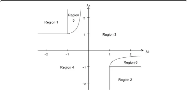
As originally indicated by Ramberg and Schmeiser (1974) and Karian and Dudewicz (2000), there are six regions of parameter values where GLD is valid, see Fig. 1. The condi-tions on the parameters and the support regions for the PDF of GLD are listed in Table 1.
Definition of T-R{generalized lambda} families of distributions
In this sub-section we define the class ofT-R{GL} families of distributions based on the quantile function of GLD.
Let Y be a random variable that follows the GLD, then the definition in (1.1) gives the CDF (in general) of the random variableXinT-R{GL} families of distributions as
FXð Þ ¼x FTðQYðFRð Þx ÞÞ ¼FT λ1þ
FRλ3ð Þx −ð1−FRð Þx Þλ4 λ2
!
: ð2:1Þ
The corresponding PDF associated with (2.1) is
fXð Þ ¼x fRð Þx λ3FR
λ3−1ð Þ þx λ
4ð1−FRð Þx Þλ4−1
λ2
!
fT λ1þ
FRλ3ð Þx −ð1−FRð ÞxÞλ4
λ2
!
: ð2:2Þ
The hazard function of the T-R{GL} families of distributions can be obtained from the definitionhX(x) =fX(x)/(1−FX(x)).
Based on the T-R{Y} framework, the link function QY: [0, 1]→[a,b], for − ∞ ≤a< b≤ ∞, is absolutely continuous and monotonic with lim
u→0þQYð Þ ¼u aand limu→1−QYð Þ ¼u b,
where [a,b] is the support of the random variableT.In other words, the choice of the ran-dom variableTis not arbitrary and it depends on the choice of the random variableYin order to have a valid distribution. Figure 1 and Table 1 show that valid GLDs are defined in different domains. Accordingly, the valid PDF ofT-R{GL} in (2.2) is associated with dif-ferent domains of the GLDs. The valid PDF’s and the associated restrictions on the pa-rameters are summarized as cases (i)-(vi) and given in Table 2.
There are good reasons to let the random variable Yin theT-R{Y} framework be the quantile function of GLD. First, adding one or more shape parameters may allow the derived distribution to have different shapes as well as being flexible enough to fit a
wide variety of data sets. Second, the support of GLD covers the three types of intervals: bounded, semi-infinite and whole real line, which places no restrictions in the process of choosing the random variable T other than those with only bounded, semi-infinite, or whole real line support. In the development of the T-R{Y} framework so far, the random variable Y has one type of support. Taking Y to be a generalized lambda random variable leads to three different types of sup-ports for the generator random variable T. By allowing one to apply different generators, T, with different supports makes the T-R{generalized lambda} a desir-able method for generating new versatile and broad generalized families of distri-butions for any given random variable R. This unique and quite attractive property of the T-R{GL} family motivates us to study this family of distributions. Similar to existing distributions, the interpretations of parameters are often appli-cation dependent. We hope that researchers in different disciplines will apply this family of distributions in their respective disciplines with specific interpretations for the parameters of the T-R{GL} distributions.
Some general properties ofT-R{generalized lambda} families of distributions
In this section, we highlight some of the general properties of theT-R{GL} families of distributions.
The following lemma shows the relationship between the random variableXthat fol-lows theT-R{GL} distributions and the random variableT.
Table 1The conditions on the parameters and the support regions of GLD (p. 39, Karian and Dudewicz (2010))
Region λ1 λ2 λ3 λ4 Q(0) Q(1)
1 all <0 <−1 >1 −∞ λ1+ (1/λ2)
5 all <0 −1<λ3<0; λ4>1 1−λ3
ð Þ1−λ3λ
4−1
ð Þλ4−1
λ4−λ3
ð Þλ4−λ3 <
−λ3 λ4 8
> > < > > :
−∞ λ1+ (1/λ2)
2 all <0 >1 <−1 λ1−(1/λ2) ∞
6 all <0 λ3>1; −1<λ4<0 1−λ4
ð Þ1−λ4ðλ3−1Þλ3−1
λ3−λ4
ð Þλ3−λ4 <
−λ4
λ3 8
> > < > >
: λ1−(1/λ2) ∞
3 all >0 >0 >0 λ1−(1/λ2) λ1+ (1/λ2)
=0 >0 λ1 λ1+ (1/λ2)
>0 =0 λ1−(1/λ2) λ1
4 all <0 <0 <0 −∞ ∞
=0 <0 λ1 ∞
<0 =0 −∞ λ1
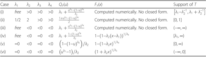
Table 2The support of the random variableTcorresponding to the cases (i)-(vi)
Case λ1 λ2 λ3 λ4 QY(u) FY(x) Support ofT
(i) free >0 >0 >0 λ1þu
λ3−ð1−uÞλ4
λ2 Computed numerically. No closed form. λ1−λ
−1 2 ;λ1þλ−21
(ii) 1/2 2 >0 >0 1þuλ3−2ð1−uÞλ4 Computed numerically. No closed form. [0, 1]
(iii) free <0 <0 <0 λ1þu
λ3−ð1−uÞλ4
λ2 Computed numerically. No closed form. (−∞,∞)
(iv) free <0 =0 <0 λ1þ1−ð1−uÞ
λ4
λ2 1−ð1−λ2ðx−λ1ÞÞ
1=λ4 [λ1,∞)
(v) =0 <0 =0 <0 1−ð1−uÞλ4=λ
2 1−ð1−λ2xÞ1=λ4 [0,∞) (vi) =0 <0 <0 =0 uλ3−1=λ
Lemma 1(Transformation): LetTbe any random variable with PDFfT(x).
a. If T has the support [λ1,∞) as in case (iv) in Table 2, then the random
variable X¼QR 1−½1−λ2ðT−λ1Þ1=λ4
belongs to the T-R{GL} families of distributions.
b. IfThas the support [0,∞) as in case (v) in Table2, then the random variableX ¼QR 1−½1−λ2T1=λ4
belongs to theT-R{GL} families of distributions.
c. IfThas the support (−∞, 0] as in case (vi) in Table2, then the random variableX ¼QR ½1þλ2T1=λ3
belongs to theT-R{GL} families of distributions.
Proof: The proof follows directly from the definition of theT-R{GL} families of distri-butions in (2.1) and Table 2.
Note that in the first three cases (i)-(iii) in Table 2, the relationships between the ran-dom variablesXandTcan be evaluated numerically.
The relation FX(x) =FT(QY(FR(x))), where T=QY(FR(X)) implies X=QR(FY(T)), provides an important connection between the random variables X and T. For ex-ample, one can apply the transformation X=QR(FY(T)) to generate random sam-ples from X which has the CDF FX(x) by first simulating the random variable T from the PDF fT(t). Moreover, the rth moments (if they exist) of theT-R{Y} family of distributions can be obtained using EX[Xr] =ET[QR(FY(T))]r.
The next lemma makes a connection between the quantile function for the random variable X which follows theT-R{GL} families of distributions and the quantile func-tions of the random variablesTandR.
Lemma 2 (Quantiles): LetQT(u) andQR(u) be the quantile functions of the random variablesTandR, respectively.
a. IfThas the support [λ1,∞) as in case (iv) in Table2, then the quantile function of
the random variableXwhich follows theT-R{GL} distributions isQXð Þ ¼u QR 1−½1−λ2ðQTð Þu −λ1Þ1=λ4
.
b. IfThas the support [0,∞) as in case (v) in Table2, then the quantile function of the random variableXwhich follows theT-R{GL} distributions isQXð Þ ¼u QR
1−½1−λ2QTð Þu1=λ4
.
c. IfThas the support (−∞, 0] as in case (vi) in Table2, then the quantile function of the random variableXwhich follows theT-R{GL} distributions isQXð Þ ¼u QR
1þλ2QTð Þu ½ 1=λ3
.
Proof: The results follow directly by solving FX(QX(u)) =u for QX(u), where FX(.) is the CDF of the random variableX.
In the literature, some of the quantile functions do not have closed form expres-sions. For instance, in the first three cases (i)-(iii) in Table 2 the random variable X has no closed form expression for its quantile function, and it has to be evalu-ated numerically.
An implicit formula for the mode(s) of the T-R{GL} families of distributions is presented in the following theorem.
fR′ð Þx fR2ð Þx ¼−Q
′
YðFRð Þx Þ
Q″YðFRð Þx Þ Q′YðFRð Þx Þ
2þ
fT′ λ1þλ2−1 FRλ3ð Þx−FRλ4ð Þx
h i
fT λ1þλ2−1 FRλ3ð Þx −FRλ4ð Þx
h i
2 4
3
5; ð3:1Þ
where FRð Þ ¼x 1−FRð Þx is the survival function of the random variable Rwith PDF
fR(x), Q′YðFRð Þx Þ ¼λ2−1 λ3FRλ3−1ð Þ þx λ4FR
λ4−1
x
ð Þ
h i
, and Q″YðFRð Þx Þ ¼λ2−1
λ3ðλ3−1ÞFRλ3−2ð Þx −λ4ðλ4−1ÞFRλ4− 2
x
ð Þ
h i
.
Proof: One can show the result in (3.1) by setting the first derivative offX(x) in (2.2) to 0.
Note that the result in Theorem 1 does not necessarily guarantee that the mode is unique. It is possible that some members of theT-R{GL} families of distributions have more than one mode. For example, the uniform-exponential{GL} distribution in section 4 is bimodal, depending on the values of its shape parameters.
Shannon (1948) defined the entropy of a random variable X as a measure of uncer-tainty variation by ηX=EX[−log(fX(X))]. The next theorem defines the Shannon’s en-tropy of the random variable X that follows theT-R{GL} families of distributions with PDFfX(x) in terms of the Shannon’s entropy of the random variableTwith PDFfT(x).
Theorem 2 The Shannon’s entropy for the T-R{GL} families of distributions is given by
ηX¼ηTþET½logfYð ÞT þET½logqRðFYð ÞT Þ; ð3:2Þ
whereηTis the Shannon’s entropy of the random variableTwith PDFfT(x) andqR(.) is
the quantile density function of the random variableR.
Proof: By the definition of Shannon’s entropy,
ηX¼EX½−logðfXð ÞX Þ ¼EX log λ3
FRλ3−1ð Þ þX λ4ð1−FRð ÞX Þλ4−1 λ2
!−1
" #
þEX½−logfRð ÞX þEX −logfT λ1þ
FRλ3ð ÞX −ð1−FRð ÞX Þλ4 λ2
!
" #
: ð3:3Þ
The random variableT ¼QYðFRð ÞX Þ ¼ λ1þFR
λ3ð ÞX−ð1−FRð ÞXÞλ4
λ2
, or equivalently,X=
QR(FY(T)). This implies that
EX −logfT λ1þ
FRλ3ð ÞX −ð1−FRð ÞX Þλ4 λ2
!
" #
¼ET½−logfTð ÞT ¼ηT; ð3:4Þ
EX log λ3
FRλ3−1ð Þ þX λ4ð1−FRð ÞX Þλ4−1 λ2
!−1
" #
¼EX½logfYðQYðFRð ÞX ÞÞ
¼ET½logfYð ÞT ; ð3:5Þ
EX½−logfRð ÞX ¼ET½−logfRðQRðFYð ÞT ÞÞ ¼ET½logqRðFYð ÞT Þ: ð3:6Þ
Substituting (3.4) through (3.6) into (3.3) gives (3.2).
+ (t/β)]−(α+ 1),t≥0,α,β> 0, and let the random variableRfollow the standard exponen-tial distribution with PDF fR(x) =e−x and quantile function QR(u) = −log(1−u). The Shannon entropy of the Lomax distribution is given by
ηT¼ððαþ1Þ=αÞ−logðα=βÞ:
ET½logfYð ÞT ¼ET log ðλ2=λ4Þð1−λ2tÞð1=λ4Þ−1
h i
¼ðλ2β λð 4−1Þ=λ4ÞΓ αð Þ2F~1ð1;1;1þα;1þλ2βÞ þ logðλ2=λ4Þ;
whereΓ(α) is the gamma function and2F~1ð1;1;1þα;1þλ2βÞis the regularized
hyper-geometric function.
ET½logqRðFYð ÞT Þ ¼ET −log 1ð −λ2tÞ1=λ4
h i
¼ð− −ð λ2βÞα=λ4ÞΓ αð Þ2F~1ðα;α;1þα;1þλ2βÞ:
Therefore, the Shannon entropy of the Lomax-exponential{GL} is given by
ηX¼ αþ1
α
−log α
β þ log λ2
λ4
þ λ2β λð 4−1Þ
λ4
Γ αð Þ2F~1ð1;1;1þα;1þλ2βÞ
− ð−λ2βÞα
λ4
Γ αð Þ2F~1ðα;α;1þα;1þλ2βÞ:
Moments In general, the non-central moments (if they exist) for theT-R{GL} family of distributions can be obtained by using EX[Xn] =ET[QR(FY(T))]n=∫T[QR(FY(t))]nfT(t)dt. However,FY(.) in the first three cases in Table 2 have no closed form and one may use EX[Xn] =∫XxnfX(x)dxto find the moments. For the cases (iv)-(vi) in Table 2, the quantile function QX(u) is in closed form, so thenth moment of the random variableX may be
obtained from EX½ ¼Xn R01½QXð Þu ndu: The following Theorem 3 derives an approxi-mation for computing thenthmoment of a member, Uniform-R{GL} of case (i).
Theorem 3 Let T be a random variable that follows the uniform distribution with support as in case (i) in Table 2,and let X be a random variable having the Uniform-R{GL} PDF. The nthmoment of X can be expressed in terms of the quantile function QR(u)and is given by:
EXð Þ ¼Xn 1 2 λ3
Z 1 0
uλ3−1Q Rð Þu
½ n
duþλ4
X∞
k¼0
−1
ð Þk λ4−1
k
Z 1 0
uk½QRð Þu ndu
" #
:
ð3:7Þ
Proof:
EX½ ¼Xn
Z ∞
−∞x
nf
Xð Þdxx ¼ 1 2
Z ∞
−∞x
nf
Rð Þx λ3FRλ3−1ð Þ þx λ4ð1−FRð Þx Þλ4−1
h i
dx: ð3:8Þ
Using the substitutionu=FR(x), then equation (3.8) can be written as
EX½ ¼Xn 1 2
Z 1 0
λ3uλ3−1½QRð Þunduþ
Z 1 0
λ4ð1−uÞλ4−1½QRð Þundu
: ð3:9Þ
1−u
ð Þλ4−1¼X
∞
k¼0
−1
ð Þk λ4−1
k
uk; ð3:10Þ
and ifλ4> 1 and it is an integer, then the upper summation stops atλ4−1. The series
in (3.10) converges uniformly on (0, 1) since 0< u < 1. By the dominated convergence theorem of series, the second integral in (3.9) can be integrated term by term. This completes the proof.
Remark 1: Letr=λ3−1 ands=λ4−1, thenthmoment ofUniform-R{GL} in (3.9) can
be expressed as the probability weighted moments of random variable R, EX½ ¼Xn 12
λ3Mn;r;0þλ4Mn;0;s
, where Mn;r;s¼ER XnFRrð ÞX FR s
X
ð Þ
is the probability weighted moments of the random variableRof order (n,r,s).
Remark 2: If the random variableRhas finite nth moment (i.e. [QR(u)]nis integrable), then by applying Cauchy-Schwarz inequality to (3.9), the nth moment ofX is bounded by the upper bound
EX½ Xn≤λ3 2
Z 1 0
QRð Þu ½ 2n
du
Z 1 0
u2λ3−2du
1=2
þλ4
2
Z 1 0
QRð Þu ½ 2n
du
Z 1 0
1−u ð Þ2λ4−2du
1=2
¼1 2 ER X
2n
1=2 λ32
2λ3−1
1=2
þ λ42
2λ4−1
1=2
" #
:
Some examples ofT-R{GL} families of distributions with differentTandR
distributions
In this section differentTandRdistributions are used to generate various members of the T-R{GL} families of distributions. We present four new T-R{GL} distributions namely, uniform-exponential{generalized lambda}, normal-uniform{generalized lambda}, Pareto-Weibull{generalized lambda} and log-logistic-logistic{generalized lambda}.
The uniform-exponential{generalized lambda} distribution
Consider case (i) in Table 2 and let T be a random variable that follows the uniform distribution. If a random variableRfollows the exponential distribution with a rate par-ameter θ> 0 and CDF FR(x) = 1−e−θx,x≥0, then the CDF and PDF of the uniform-exponential{generalized lambda}(U-E{GL}) distribution are given by, respectively:
FXð Þ ¼x 1
2 1þ 1−e
−θx
λ3
−e−θx λ4
h i
; ð4:1Þ
fXð Þ ¼x 1 2θe
−θx λ
3 1−e−θx
λ3−1
þλ4 e−θx
λ4−1
h i
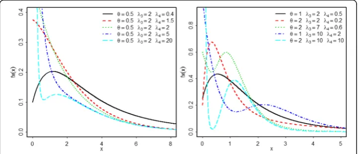
;x≥0;θ;λ3;λ4>0: ð4:2Þ
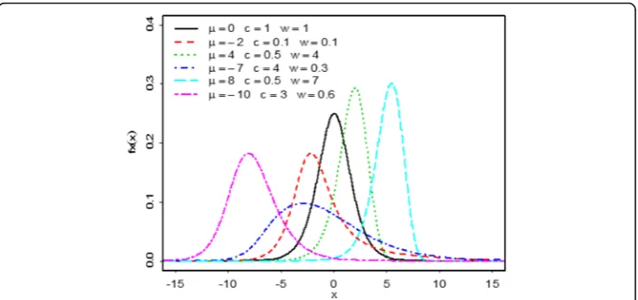
The parameters λ3andλ4are shape parameters (see Figure 2). It is clear that the
U-E{GL} distribution reduces to the exponential distribution whenλ3=λ4= 1 orλ3=λ4=
2. Various shapes of the U-E{GL} distribution for different values of the parameters θ,
λ3,λ4are provided in Fig. 2. These graphs indicate that theU-E{GL} distribution can be
The normal-uniform{generalized lambda} distribution
Consider case (iii) in Table 2 and letTbe a standard normal random variable with PDF fTð Þ ¼x ϕð Þ ¼x 1ffiffiffiffi
2π
p expð−x2=2Þand CDFF
T(x) =Φ(x). LetRbe a random variable that follows the uniform distribution with parameters a,b and CDF FRð Þ ¼x x−a
b−a; x∈[a,b], − ∞ <a<b<∞. If we set the location parameterλ1= 0 in case (iii) in Table 2, then the
CDF and PDF of the normal-uniform{generalized lambda} (N-U{GL}) distribution are given by, respectively:
FXð Þ ¼x Φ 1 λ2
x−a b−a
λ3
− 1−x−a b−a
λ4
; ð4:3Þ
fXð Þ ¼x 1 λ2ðb−aÞ
ffiffiffiffiffiffi
2π p λ3
x−a b−a
0 @
1 A
λ3−1
þλ4 1−
x−a b−a
0 @
1 A
λ4−1
0 B @ 1 C A
exp − 1 2λ22
x−a b−a
0 @
1 A
λ3
− 1−x−a b−a
0 @ 1 A λ4 0 B @ 1 C A 2 2 6 4 3 7
5;x∈½a;b;−∞<a<b<∞;λ2;λ3;λ4<0:
ð4:4Þ
The parametersλ2,λ3, andλ4are shape parameters (see Fig. 3). Plots ofN-U{GL}
dis-tribution when a= 0,b= 3 and various values of λ2,λ3andλ4are given in Fig. 3. The
plots show that the N-U{GL} distribution can be symmetric, left skewed or right skewed and it can be either unimodal or bimodal.
The Pareto-Weibull{generalized lambda} distribution:
Consider case (iv) in Table 2 and let the random variableTfollow the Pareto distribu-tion with CDFFT(x) = 1−(λ1/x)s,x≥λ1,λ1> 0,s> 0, and take the random variableRto
be the Weibull distribution with CDF FRð Þ ¼x 1−e−ðx=γÞc;x≥0;γ;c>0: If we replace
λ1λ2 by −β,β> 0 and let λ4= −1, then the CDF and PDF of the
Pareto-Weibull{generalized lambda} (P-W{GL}) distribution are respectively given by
FXð Þ ¼x 1− β= β−1þeðx=γÞ c
h i
s
; ð4:5Þ
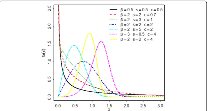
fXð Þ ¼x scβsγ−1ðx=γÞc−1eðx=γÞcβ−1þeðx=γÞc−s−1;x≥0;s;β;c;γ>0: ð4:6Þ
When s=β= 1, theP-W{GL} distribution reduces to the Weibull distribution, which has Rayleigh and exponential distributions as special cases. It is worth mentioning that by setting c= 1 in (4.6), the P-W{GL} distribution reduces to the Pareto-exponential{generalized lambda} distribution, which is called in the literature the gamma/Gompertz distribution. Thus, the P-W{GL} distribution is a generalization of the gamma/Gompertz distribution, which was derived using a different approach (Bemmaor and Glady, 2012).
Figure 4 illustrates some possible shapes of the density function in (4.6) when γ= 1 and for selected parameter values. The graphs in Fig. 4 indicate that the P-W{GL} dis-tribution can be skewed to the left, skewed to the right or monotonically decreasing (reversed J-shape). Different combinations of the values of the parameters were tried but in all cases the graph ofP-W{GL} distribution appears to be unimodal.
Fig. 3Plots ofN-U{GL} distribution whena= 0,b= 3 and for various values ofλ2,λ3andλ4
The log-logistic-logistic{generalized lambda} distribution:
Consider case (v) in Table 2 and let Tbe a random variable that follows the standard log-logistic distribution with CDFFTð Þ ¼x 1þxx;x≥0. Take the random variableRto be
the logistic distribution with CDF FRð Þ ¼x 12þ12tanh x2−σμ
¼ eðx−μÞ=σ
1þeðx−μÞ=σ;−∞<x<∞;
where the location parameter μ∈ℝ and the scale parameter σ> 0. If we replace λ2by −c,c> 0 and λ4 by −w,w> 0, then the CDF and PDF of the
log-logistic-logistic{generalized lambda} (LL-L{GL}) distribution are respectively given by
FXð Þ ¼x
1−2wð1−tanh½ðx−μÞ=2σÞ−w
1−c−2wð1−tanh½ðx−μÞ=2σÞ−w; ð4:7Þ
fXð Þ ¼x cwð2−2 tanh½ðx−μÞ=2σÞÞ w−1
sech2½ðx−μÞ=2σÞ σf2wþðc−1Þð1−tanh½ðx−μÞ=2σÞÞwg2 ;
−∞<x<∞;μ∈ℝ;σ;c;w>0: ð4:8Þ
Note that the LL-L{GL} distribution reduces to the logistic distribution whenc=w= 1. In Fig. 5, various graphs of the density in (4.8) when σ= 1 and for various values of the parameters μ,cand ware provided. The plots show that the LL-L{GL} distribution can be symmetric, left skewed or right skewed. The graph ofLL-L{GL} distribution ap-pears to be unimodal from trying many different combinations of the parameter values.
Parameter estimation and simulation for U-E{GL} distribution
In this section, we use the method of maximum likelihood to address the parameter es-timation and conduct a simulation to examine the performance of this method. Let x1,
x2,…,xnbe a random sample of sizenfrom aU-E{GL} distribution defined in equation (4.2), then the log-likelihood function is given by
ℓðθ;λ3;λ4Þ ¼nlogðθ=2Þ−θX
n
i¼1 xiþX
n
i¼1
log λ31−e−θxi λ3−1þλ4e−θxi λ4−1
h i
: ð5:1Þ
To measure the performance of the MLEs, we conduct a simulation study to evaluate the MLEs in terms of the bias (actual−estimate) and standard deviation of the param-eter estimates for different paramparam-eter combinations and sample sizes.
The U-E{GL} is a generalization of the exponential distribution. It reduces to the ex-ponential distribution with mean 1/θ when λ3=λ4= 1 orλ3=λ4= 2. In the simulation
study, we take the initial estimates of parameters λ3andλ4to be 1 and the initial
esti-mate of parameterθ to be the MLE ofθby taking the simulated data to have an expo-nential distribution. We obtain a random sample x1,x2,…,xnof size nfrom aU-E{GL} distribution by first generating a random sample t1,t2,…,tn from standard uniform distribution and then transforming it to U-E{GL} using the relationship X=QR(FY(T)) = −(1/θ) log(1−FY(T)), where FY(T) is computed numerically in SAS for different parameter combinations ofλ3andλ4.
In this simulation, five sample sizes are considered (n= 50, 100, 250, 500, 1000). The NLMIXED procedure in SAS is used to maximize the log-likelihood function in Equa-tion (5.1). We consider different parameter combinaEqua-tions to cover different shapes of the distribution, including monotonically decreasing, right skewed, unimodal or bi-modal. The parameter combinations considered are (λ3,λ4,θ) = {(0.8, 0.6, 0.5), (1, 2,
2), (2, 0.8, 1), (3, 0.5, 3), (4, 0.7, 2)}. The MLEs of the parameters λ3,λ4 and θ are
com-puted and the process is repeated 1000 times for each sample size and each parameter
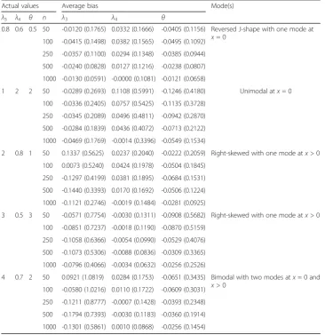
Table 3Average bias (standard deviation) for the MLEs
Actual values Average bias Mode(s)
λ3 λ4 θ n λ3 λ4 θ
0.8 0.6 0.5 50 -0.0120 (0.1765) 0.0332 (0.1666) -0.0405 (0.1156) Reversed J-shape with one mode at
x= 0 100 -0.0415 (0.1498) 0.0382 (0.1565) -0.0495 (0.1092)
250 -0.0357 (0.1100) 0.0294 (0.1348) -0.0385 (0.0944)
500 -0.0240 (0.0828) 0.0127 (0.1216) -0.0238 (0.0807)
1000 -0.0130 (0.0591) -0.0000 (0.1081) -0.0121 (0.0658)
1 2 2 50 -0.0289 (0.2693) 0.1108 (0.5991) -0.1246 (0.4180) Unimodal atx= 0
100 -0.0336 (0.2405) 0.0757 (0.5425) -0.1135 (0.3728)
250 -0.0345 (0.2089) 0.0496 (0.4811) -0.0942 (0.2870)
500 -0.0284 (0.1839) 0.0436 (0.4072) -0.0713 (0.2122)
1000 -0.0469 (0.1769) -0.0014 (0.3396) -0.0549 (0.1534)
2 0.8 1 50 0.1337 (0.5625) 0.0237 (0.2040) -0.0222 (0.2059) Right-skewed with one mode atx> 0
100 0.0073 (0.5240) 0.0424 (0.1978) -0.0504 (0.1845)
250 -0.1297 (0.4199) 0.0381 (0.1895) -0.0684 (0.1531)
500 -0.1440 (0.3393) 0.0170 (0.1692) -0.0506 (0.1224)
1000 -0.1121 (0.2746) -0.0019 (0.1484) -0.0281 (0.0925)
3 0.5 3 50 -0.0571 (0.7754) -0.0030 (0.1311) -0.0908 (0.5682) Right-skewed with one mode atx> 0
100 -0.0851 (0.7237) -0.0018 (0.1190) -0.0870 (0.5159)
250 -0.1058 (0.6366) -0.0054 (0.0990) -0.0529 (0.4076)
500 -0.1073 (0.5306) -0.0088 (0.0836) -0.0309 (0.3365)
1000 -0.0796 (0.4066) -0.0034 (0.0632) -0.0256 (0.2526)
4 0.7 2 50 0.0921 (1.0819) 0.0284 (0.1753) -0.0651 (0.3435) Bimodal with two modes atx= 0 and
x> 0 100 -0.0580 (1.0216) 0.0110 (0.1722) -0.0609 (0.3031)
250 -0.1211 (0.8777) -0.0007 (0.1428) -0.0393 (0.2348)
500 -0.1794 (0.7393) -0.0030 (0.1183) -0.0360 (0.1914)
combination. The average bias and standard deviation of the MLEs are computed and the results are presented in Table 3.
The simulation results show that the maximum likelihood estimation method per-forms quite well in estimating the U-E{GL} distribution parameters. It is observed that the standard deviations of the MLEs decrease as the sample size increases and the aver-age biases of the MLEs are somewhat small and seem to be reasonable. As the sample size increases, it is also noticed that the average biases do not show a clear decreasing or increasing pattern. In addition, it appears that the MLEs of θ tend to be overesti-mated. In conclusion, the simulation results suggest that the maximum likelihood estimation method is appropriate and it can be used to estimate the parameters of the U-E{GL} distribution.
Applications
In order to illustrate the flexibility of the members of T-R{GL} families of distributions in fitting real data, we present some applications of theU-E{GL} distribution using two different real data sets. We use the method of maximum likelihood to estimate the pa-rameters of the fitted distribution. The fits of theU-E{GL} distribution are compared to other distributions based on the log-likelihood value, the Kolmogorov-Smirnov (K-S) statistic, thep-value of (K-S) statistic and the Akaike information criterion (AIC).
Remission times of bladder cancer patients:
The data in Table 4 represents the remission times (in months) of a random sample of 128 bladder cancer patients. This data was previously used by Zea et al. (2012) to com-pare the fits of the five-parameter beta exponentiated Pareto (BEP) distribution and other sub-models such as the beta-Pareto (BP) distribution. The data is also recently studied and analyzed by Almheidat et al. (2015) to show the flexibility of the four-parameter Cauchy-Weibull{logistic} (C-W{L}) distribution in fitting real data. The data is unimodal and is highly skewed to the right (skewness = 3.286 and kurtosis = 18.483). We apply the U-E{GL} distribution to fit the same data. The MLEs (with corresponding standard errors) of the parameters, the log-likelihood, the AIC, the K-S statistic and thep-value of (K-S) statistic for theU-E{GL} distribution and the other fitted distributions are provided in Table 5. The results in Table 5 for the C-W{L} distribution are taken from Almheidat et al.
Table 4Remission times (in months) of bladder cancer patients
0.080 0.200 0.400 0.500 0.510 0.810 0.900 1.050 1.190 1.260 1.350 1.400
1.460 1.760 2.020 2.020 2.070 2.090 2.230 2.260 2.460 2.540 2.620 2.640
2.690 2.690 2.750 2.830 2.870 3.020 3.250 3.310 3.360 3.360 3.480 3.520
3.570 3.640 3.700 3.820 3.880 4.180 4.230 4.260 4.330 4.340 4.400 4.500
4.510 4.870 4.980 5.060 5.090 5.170 5.320 5.320 5.340 5.410 5.410 5.490
5.620 5.710 5.850 6.250 6.540 6.760 6.930 6.940 6.970 7.090 7.260 7.280
7.320 7.390 7.590 7.620 7.630 7.660 7.870 7.930 8.260 8.370 8.530 8.650
8.660 9.020 9.220 9.470 9.740 10.06 10.34 10.66 10.75 11.25 11.64 11.79
11.98 12.02 12.03 12.07 12.63 13.11 13.29 13.80 14.24 14.76 14.77 14.83
15.96 16.62 17.12 17.14 17.36 18.10 19.13 20.28 21.73 22.69 23.63 25.74
(2015) whereas the results for the BP and BEP distributions are obtained from Zea et al. (2012). The other results in Table 5 are obtained by using the SAS (PROC NLMIXED) software.
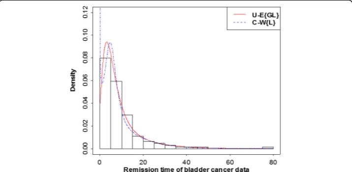
The values in Table 5 indicate that the three-parameter U-E{GL} distribution outper-forms the other three distributions and provide the best fit (based on the log-likelihood, the AIC, the K-S statistic and thep-value of K-S statistic) to the remission times of bladder cancer patient’s data. This application suggests that theU-E{GL} distribution can fit very well highly right skewed data with long tail. Figure 6 displays the histogram of the data and the density functions of the fitted distributions that provide adequate fits to the data.
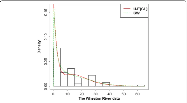
The Wheaton river data
In Table 6, the data set with n= 72 is on exceedances (in m3/s) of flood peaks of the Wheaton River, Yukon Territory, Canada, for the years 1958 to 1984, rounded to one decimal place. This data was considered by Akinsete et al. (2008) to illustrate the appli-cation of the beta-Pareto (BP) distribution. The data is also used by Alshawarbeh et al. (2013) and fitted to the beta-Cauchy (BC) distribution. Recently, Al-Aqtash et al.
Fig. 6The histogram and the fitted PDFs for remission times of bladder cancer patient’s data
Table 5MLEs for remission times of bladder cancer patient’s data (standard errors in parentheses)
Distribution aBP aBEP bFour-parameter
C-W{L}
U-E{GL}
Parameter estimates a¼4:805 (0.055)
b¼100:502 (0.251)
k¼0:011 (0.001) β¼0:080
a¼0:348 (0.097)
b¼159831 (183.7501)
k¼0:051 (0.019) β¼0:080 α¼8:612 (2.093)
α¼−2:3040 (1.0937) β¼2:0205 (0.4585)
k¼3:0673 (0.7319) λ¼12:663 (2.6326)
θ¼0:2757 (0.0665) λ3¼2:5904 (0.9285) λ4¼0:2894 (0.0858)
Log-likelihood −480.446 −432.41 −416.0965 −409.45
AIC 968.893 874.819 840.2 824.9
K-S statistic (p-value)
0.217 (1.105E-5)
0.142 (0.0121)
0.06672 (0.6189)
0.02876 (0.9999)
a
MLEs, log likelihood, K-S (p-value), and AIC are from Zea et al. (2012). b
(2015) used the data in an application of the Gumbel-Weibull (GW) distribution. The data is skewed to the right (skewness = 1.5 and kurtosis = 3.19).
To show the applicability of theU-E{GL} distribution, the distribution is applied to fit the data set and the results are compared with the BP distribution, the BC distribution and GW distribution. The maximum likelihood estimates, the log-likelihood value, the AIC, the K-S test statistic, and the p-value of the K-S statistics for the fitted distribu-tions are presented in Table 7. The MLEs, the values of the K-S statistic and its corre-sponding p-value for the BP distribution, the BC distribution, and GW distribution in Table 7 are obtained from Al-Aqtash et al. (2015).
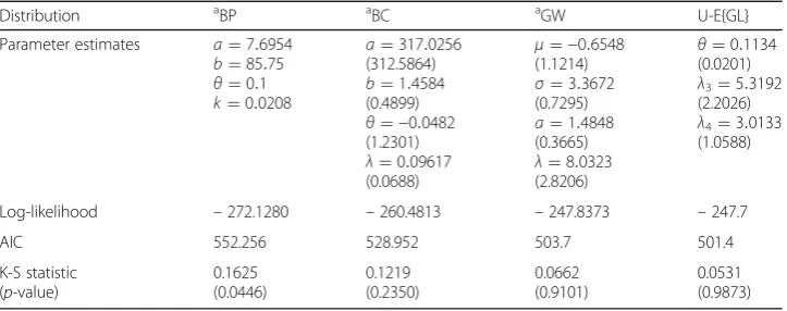
Based on the p-value of K-S statistic, the results in Table 7 show that the U-E{GL} distribution and GW distribution are superior to the other two distributions. Among the fitted distributions, it seems that the U-E{GL} provides the best fit to the data with smallest AIC, K-S statistic, and largest log-likelihood value. Figure 7 provides the histo-gram of the data and the density functions of theU-E{GL} and GW distributions.
From sub-sections 6.1 and 6.2, we observe that the U-E{GL} distribution seems to be very competitive to other distributions in fitting highly right skewed data with long tail.
Summary
In this article, the class of T-R{generalized lambda} families of distributions based on the quantile of generalized lambda distribution is introduced using the T-R{Y} frame-work. One of the advantages for letting the random variableYin theT-R{Y} framework to be the quantile function of GLD is that the generalized lambda random variable leads to three different types of support as shown in sub-section 2.2. For this reason, different families of theT-R{generalized lambda} distributions can be derived based on the choices of the random variablesTand R. Some general properties of T-R{general-ized lambda} families of distributions are studied.
Table 7Parameter estimates for Wheaton river data (standard errors in parentheses)
Distribution aBP aBC aGW U-E{GL}
Parameter estimates a¼7:6954
b¼85:75 θ¼0:1
k¼0:0208
a¼317:0256 (312.5864)
b¼1:4584 (0.4899) θ¼−0:0482 (1.2301) λ¼0:09617 (0.0688)
μ¼−0:6548 (1.1214) σ¼3:3672 (0.7295)
a¼1:4848 (0.3665) λ¼8:0323 (2.8206)
θ¼0:1134 (0.0201) λ3¼5:3192 (2.2026) λ4¼3:0133 (1.0588)
Log-likelihood –272.1280 –260.4813 –247.8373 –247.7
AIC 552.256 528.952 503.7 501.4
K-S statistic (p-value)
0.1625 (0.0446) 0.1219 (0.2350) 0.0662 (0.9101) 0.0531 (0.9873) a
MLEs, K-S statistic (p-value) are from Al-Aqtash et al. (2015).
Table 6Exceedances of the Wheaton River data.
Four new generalizedR distributions in theT-R{generalized lambda} families of dis-tributions are defined, namely, the uniform-exponential{generalized lambda}, the normal-uniform{generalized lambda}, the Pareto-Weibull{generalized lambda} and the log-logistic-logistic{generalized lambda}. As mentioned in sub-section 4.3, the Pareto-Weibull{generalized lambda} distribution has the gamma/Gompertz distribution and other distributions as special cases.
The uniform-exponential{generalized lambda} distribution is applied to fit two real data sets. The results show that the uniform-exponential{generalized lambda} distribu-tion has the ability to fit right skewed data with long tail.
Acknowledgments
We are grateful for many constructive comments and suggestions from the handling editor and the reviewer. These comments and suggestions have greatly improved the presentation of the paper.
Funding
The third author (Felix Famoye) gratefully acknowledges the financial support received from the U.S. Department of State, Bureau of Education and Cultural Affairs under the Fulbright Grant # PS00230565.
Authors’contributions
The authors, viz MA, CL and FF with the consultation of each other carried out this work and drafted the manuscript together. All authors read and approved the final manuscript. The authors confirmed that the content of the manuscript has not been published, or submitted for publication elsewhere.
Competing interests
The authors declare that they have no competing interests.
Publisher’s Note
Springer Nature remains neutral with regard to jurisdictional claims in published maps and institutional affiliations.
Received: 7 June 2017 Accepted: 27 October 2017
References
Akinsete, A., Famoye, F., Lee, C.: The beta-Pareto distribution.Statistics.42(6), 547–563 (2008)
Al-Aqtash, R., Famoye, F., Lee, C.: On generating a new family of distributions using the logit function.Journal of Probability and Statistical Science.13(1), 135–152 (2015)
Aljarrah, M.A., Lee, C., Famoye, F.: On generatingT-Xfamily of distributions using quantile functions.Journal of Statistical Distributions and Applications.1, 1–17 (2014)
Almheidat, M., Famoye, F., Lee, C.: Some generalized families of Weibull distribution: Properties and applications.
International Journal of Statistics and Probability.4, 18–35 (2015)
Alshawarbeh, E., Famoye, F., Lee, C.: Beta-Cauchy distribution: some properties and applications.Journal of Statistical Theory and Applications.12(4), 378–391 (2013)
Alzaatreh, A., Famoye, F., Lee, C.: Gamma-Pareto distribution and its applications.Journal of Modern Applied Statistical Methods.11(1), 78–94 (2012)
Alzaatreh, A., Lee, C., Famoye, F.: A new method for generating families of continuous distributions.Metron.71(1), 63– 79 (2013)
Alzaatreh, A., Lee, C., Famoye, F.:T-normal family of distributions: a new approach to generalize the normal distribution.
Journal of Statistical Distributions and Applications.1, 1–16 (2014)
Bemmaor, A.C., Glady, N.: Modeling purchasing behavior with sudden“Death”: A flexible customer lifetime model.
Management Science.58(5), 1012–1021 (2012)
Cordeiro, G.M., de Castro, M.: A new family of generalized distributions.Journal of Statistical Computation and Simulation.81(7), 883–898 (2011)
Cordeiro, G.M., Ortega, E.M.M., Nadarajah, S.: The Kumaraswamy Weibull distribution with application to failure data.
Journal of the Franklin Institute.347, 1399–1429 (2010)
de Santana, T.V.F., Ortega, E.M., Cordeiro, G.M., Silva, G.O.: The Kumaraswamy-log-logistic distribution.Journal of Statistical Theory and Applications.3, 265–291 (2012)
Eugene, N., Lee, C., Famoye, F.: Beta-normal distribution and its applications.Communications in Statistics-Theory and Methods.31(4), 497–512 (2002)
Famoye, F., Lee, C., Olumolade, O.: The beta-Weibull distribution.Journal of Statistical Theory and Applications.4(2), 121– 136 (2005)
Jones, M.C.: Kumaraswamy’s distribution: A beta-type distribution with tractability advantages.Statistical Methodology.6, 70–81 (2009)
Karian, Z.A., Dudewicz, E.J.:Fitting statistical distributions: the generalized lambda distribution and generalized bootstrap methods. Chapman and Hall/CRC Press, Boca Raton, FL (2000)
Karian, Z.A., Dudewicz, E.J.:Handbook of fitting statistical distributions with R. Chapman and Hall/CRC Press, Boca Raton, FL (2010)
Kumaraswamy, P.: A generalized probability density function for double-bounded random processes.Journal of Hydrology.46, 79–88 (1980)
Lee, C., Famoye, F., Alzaatreh, A.: Methods for generating families of univariate continuous distributions in the recent decades,WIREs.Computational Statistics.5(3), 219–238 (2013)
Nadarajah, S., Kotz, S.: The beta exponential distribution.Reliability Engineering and System Safety.91(6), 689–697 (2006) Paranaíba, P.F., Ortega, E.M., Cordeiro, G.M., Pascoa, M.A.D.: The Kumaraswamy Burr XII distribution: theory and practice.
Journal of Statistical Computation and Simulation.83(11), 2117–2143 (2013)
Pereira, M.B., Silva, R.B., Zea, L.M., Cordeiro, G.M.: The Kumaraswamy Pareto distribution.Journal of Statistical Theory and Applications.12(2), 129–144 (2012)
Ramberg, J.S., Schmeiser, B.W.: An approximate method for generating asymmetric random variables.Communications of the ACM.17(2), 78–82 (1974)
Shannon, C.E.: A mathematical theory of communication.Bell System Technical Journal.27, 379–432 (1948)
Tukey, J.W.: The practical relationship between the common transformations of percentages of counts and of amounts,
Technical Report 36.Princeton University,Statistical Techniques Research Group(1960)