http://www.sciencepublishinggroup.com/j/ijssam doi: 10.11648/j.ijssam.20180302.14
ISSN: 2575-5838 (Print); ISSN: 2575-5803 (Online)
Efficiency Comparisons of Different Estimators for Panel
Data Models with Serially Correlated Errors: A Stochastic
Parameter Regression Approach
Mohamed Reda Abonazel
Department of Applied Statistics and Econometrics, Institute of Statistical Studies and Research, Cairo University, Cairo, Egypt
Email address:
To cite this article:
Mohamed Reda Abonazel. Efficiency Comparisons of Different Estimators for Panel Data Models with Serially Correlated Errors: A Stochastic Parameter Regression Approach. International Journal of Systems Science and Applied Mathematics.
Vol. 3, No. 2, 2018, pp. 37-51. doi: 10.11648/j.ijssam.20180302.14
Received: June 5, 2018; Accepted: June 25, 2018; Published: July 25, 2018
Abstract:
This paper considers panel data models when the errors are first-order serially correlated as well as with stochastic regression parameters. The generalized least squares (GLS) estimators for these models have been derived and examined in this paper. Moreover, an alternative estimator for GLS estimators in small samples has been proposed, this estimator is called simple mean group (SMG). The efficiency comparisons for GLS and SMG estimators have been carried out. The Monte Carlo studies indicate that SMG estimator is more reliable in most situations than the GLS estimators, especially when the model includes one or more non-stochastic parameter.Keywords:
First-Order Serial Correlation, Mixed-Stochastic Parameter Regression, Negative Variances, Pooled Least Squares, Simple Mean Group, Swamy’s Test1. Introduction
In panel data models, the pooled least squares estimator is the best linear unbiased estimator (BLUE) under the classical assumptions as in the general linear regression model. These assumptions are discussed in [1, 2]. An important assumption for panel data models is that the individuals in the database are drawn from a population with a common regression parameter vector. In other words, the parameters of a classical panel data model must be non-stochastic. In particular, this assumption is not satisfied in most economic models, see, e.g., [3, 4]. In this paper, panel data models are studied when this assumption is relaxed. In this case, the model is called stochastic parameter regression (SPR) model. This model has been examined in several publications such as [5-13]. Some statistical and econometric publications refer to this model as Swamy’s model, e.g., [14-18].
In SPR model, Swamy [5] assumed that the individuals in the database are drawn from a population with a common regression parameter, which is a non-stochastic component, and a stochastic component, that will allow the parameters to differ from unit to unit. This model has been developed by
many researchers, see, e.g., [19-21].
Generally, the SPR models have been applied in several fields, especially in finance and economics, and they constitute a unifying setup for many statistical problems. For example, Boot and Frankfurter [22] used the SPR model to examine the optimal mix of short and long-term debt for firms. Feige and Swamy [23] applied this model to estimate demand equations for liquid assets, while Boness and Frankfurter [24] used it to examine the concept of risk-classes in finance. Recently, Westerlund and Narayan [25] used the stochastic parameter approach to predict the stock returns at the New York Stock Exchange.
The main objective of this paper is to provide the researcher with some guidelines on how to select the appropriate estimator of panel data models when the parameters are stochastic and mixed-stochastic. To achieve this objective, the conventional estimators of these models in small samples are examined. Also, an alternative consistent estimator of these models has been proposed under an assumption that the errors are first-order serially correlated.
of the parameters of the model are stochastic. Section 3 presents an appropriate estimator when the parameters are mixed-stochastic. In section 4, an alternative estimator of these models has been proposed. Section 5 contains the results of Monte Carlo simulation studies. Finally, section 6 offers the concluding remarks.
2. The Model with Stochastic Parameters
Let there be observations for cross-sectional units over
time periods. Suppose the variable for the th unit at time
is specified as a linear function of strictly exogenous
variables, , in the following form:
= ∑ + = x + , = 1, … , ; = 1, … , , (1)
where denotes the random error term, x is a 1 ×
vector of exogenous variables, and is the × 1 vector of
regression parameters. Stacking (1) over time:
= + , (2)
where = , , … , , = x , x , … , x , =
, … , , and = , … , . Model assumptions:
Assumption 1: The errors have zero mean, i.e., =
0; ∀ = 1, … , .
Assumption 2: The errors have a constant variance for each individual but they are cross-sectional heteroscedasticity
as well as they are first-order serially correlated: =
$ , % + & ; |$ | < 1, where $ for = 1, … , are
first-order serial correlation coefficients and are fixed. Where
& = 0, ) , % &* + = 0; ∀ , ,, and . And
)& &*-+ = ./0 4 ℎ678 3601 2 = 3; = , , , = 1, … , ; , 3 = 1, … , ,
it is assumed that in the initial time period the errors have the same properties as in subsequent periods. So, assume that:
9 = /01⁄1 − $ ; ∀ .
Assumption 3: The exogenous variables are non-stochastic (in repeated samples), and then assume independent with
other variables in the model. And the value of 7<=> =
; ∀ = 1, … , , where < , .
Assumption 4: The vector of regression parameters is specified as: = ̅ + @ , where ̅ = ) ̅ , … , ̅ + is a vector
of non-stochastic parameter and @ = @ , … , @ is a
vector of random variables with zero means and constant variance-covariances:
@ = 0; )@ @*+ = .A
∗ 2 = ,
0 2 ≠ , , , = 1, … , ,
where A∗= D <EFG H; for > = 1, . . , . And assume also that
)@ * + = 0 ∀ and ,.
Using assumption 4, the model in (2) can be rewritten as:
L = ̅ + 6; 6 = M@ + , (3)
where L = , , … , N , = , , … , N , =
, … , N , @ = @ , … , @N , and M = D <EF H; for
= 1, … , . Under assumptions 1 to 4, the BLUE of ̅ and the variance-covariance matrix of it are:
̅O
PQRPS= T∗% % T∗% L;
U<7 V ̅OPQRPSW = T∗% % = X∑ YA∗+ /01 Ω% % [
%
N \% , (4)
where T∗= ] + M ^N⨂A∗ M , with
] =
` a
b/0c0Ω /0e0Ω ⋯⋱ 0⋮
⋮ ⋱ ⋱ 0
0 ⋯ 0 /0hΩNNi
j k
,
and
A∗ = l
N% V∑ ∗ ∗
m
N −
N∑N ∗∑ ∗
m
N Wn −
N∑ /N 01 Ω% % , (5)
where ∗= Ω% % Ω% , with
Ω = %o
1 e
` b
1 $ $ ⋯ $ %
$ 1 $ ⋯ $ %
⋮ ⋮ ⋮ ⋱ ⋮
$ % $ % $ %p ⋯ 1 i
k.
It is noted that the PQRPS̅O can be rewrite as a weighted average of GLS estimator for each cross-sectional unit:
̅O
PQRPS= ∑ qN ∗ ∗, (6)
where
q∗= X∑ YA∗+ /0
1 Ω% % [
%
N \%
X∑ YA∗+ /0
1 Ω% % [
%
N \.
To make the PQRPS̅O estimator feasible, we suggest using the following consistent estimators for $and /01:
$r =∑wuxest1ust1,uvc
∑wuxest1,uvce ; /y01 =
0y1m0y1
% , (7)
where y = y , … , y = − O; O = % ,
&̂ = y − $r y, % for = 2, … , . 1
By replacing $ by $r in Ω matrix, it gives consistent
estimators of Ω , say Ω€ . Use of /y01and Ω€ to get consistent estimators of ] and A∗, say ]r and Ar∗. By using consistent estimators (/y01,Ω€ , and Ar∗), it gives a consistent estimator of
T∗, say TO∗. And then use TO∗ to get a feasible estimator of
̅O
PQRPS.
Note that in non-stochastic parameter model, we assume that the errors are cross-sectional heteroskedasticity as well as they are first-order serially correlated. However, the individuals in the database are drawn from a population with
a common regression parameter vector ̅, i.e., = ⋯ =
N= ̅. Therefore the BLUE of ̅, under assumptions 1 to 3,
is:
̅O
Q•P= ]% % ]% L ,
this estimator has been termed pooled least squares (PLS) estimator. Using ]r that defined above, it gives the feasible (FPLS) estimator of PLS.
In standard stochastic parameter model that presented by Swamy [5], he assumed that the errors are cross-sectional heteroscedasticity and they are serially independently. As for the parameters, he assumed the same conditions in
assumption 4. Therefore, the BLUE of ̅, under Swamy’s [5]
assumptions, is:
̅O
PQR = T% % T% L,
where T = ‚ƒ⨂^ + M ^N⨂A M , with ‚ƒ= D <EF/ H;
for = 1, . . , , / = U<7 , and
A = lN% V∑N −
N∑N ∑N Wn −
lN∑ /N % n.
To make the PQR̅O estimator feasible, Swamy [27] used the
following unbiased and consistent estimator for / :
/y =st1mst1
% ,
where y is defined in (7). Swamy [6, 7] showed that PQR̅O estimator, under Swamy’s [5] assumptions, is consistent as
both , → ∞ and is asymptotically efficient as → ∞.
It is worth noting that, just as in the error-components model, the estimates values of A∗ and A are not necessarily non-negative definite. So, expect to obtain the negative values of the estimated variances of PQRPS̅O and PQR̅O . To avoid this problem, it can use the following consistent estimators for A∗ and A:
Ar∗† =
N% V∑ O∗O∗
m
N −
N∑N O∗∑ O∗
m
N W,
Ar†=
N% V∑N O O −N∑N O ∑N O W.
1 The estimator of $ in (7) is consistent, but it is not unbiased. See [26] for other suitable consistent estimators of it that are often used in practice.
Swamy [5] suggested use Ar† if one finds the estimated variance of PQR̅O is negative.2 Although that these estimators
Ar∗† and Ar†) are biased but they are non-negative definite
and consistent when → ∞, see [16, 28]. Moreover, these
estimators may be suitable in case of moderate or large samples but they are not suitable for small samples.
3. The Model with Mixed-Stochastic
Parameters
In this section, the GLS estimator for the model with mixed (stochastic and non-stochastic) parameters will be derived. In this case, the (mixed SPR) model can be written as:
= + + = ‡ ˆ + , (8)
where and are defined in (2), ‡ = , where
and are × and × matrices of observations on
and explanatory variables, respectively. ˆ =
, , where is a × 1 vector of parameters
assumed to be stochastic with mean ̅ and
variance-covariance matrix A‰ , and is a × 1 vector of
parameters assumed to be non-stochastic, where + =
. The model in (8) applies to each of cross-sections.
Under suppose that = ̅ + @‰ , these individual
equations can be combined as:
L = ‡ˆŠ + ‹, (9)
where L is defined in (3), ‡ = ‡ , … , ‡N , ˆŠ = ) ̅ , +, and ‹ = ‹ , … , ‹N , where ‹ = @‰ + .
Under Swamy’s [5] assumptions, this model has been examined by Swamy [27] and Rosenberg [30]. However, in this paper, this model under assumptions (1 to 4) will be
examined, therefore the variance-covariance matrix of ‹ is:
‹ ‹ = ] + M‰c)^N⨂A‰c+M‰c = Π,
where
M‰c= •
0 ⋯ 0
0 ⋯ 0
⋮ ⋮ ⋱ ⋮
0 0 ⋯ N
Ž.
The GLS estimator of ˆŠ is:
ˆŠr•PQRPS= ‡ Π% ‡ % ‡ Π% L =
• ΠΠ%% ΠΠ%% ‘% • ΠΠ%% LL‘, (10)
Where = , … , N and = , … , N .
Since the mixed SPR model is a special case of the SPR model when the variances of certain parameters are assumed to be equal to zero, therefore it can get the feasible estimator
for ˆŠr by the following algorithm:
Step 1: Calculate Ar∗ as in (5), by using consistent
estimators of /01 and Ω as given in (7).
Step 2: Find the estimation of A‰ , say Ar‰ , by removing the rows and columns for non-stochastic parameter (that within vector) from Ar∗ matrix.
Step 3: Find the estimation of Π, say Π€, by using Ar‰ and consistent estimators in (7).
Step 4: Finally, using Π€ in (10) to get the feasible estimator for ˆŠr.
The main point in this algorithm is step 2, i.e., how determine the non-stochastic parameters in the model. It needs to a statistical test for randomness of parameters. In this paper, Swamy’s [5] test will be used. The basic idea of this test; since @ is fixed for every , as given in assumption 4, so it becomes possible to test of random variation indirectly by testing whether or not the non-stochastic
parameters vectors are all equal. That is, the null
hypothesis is:
’9: = ⋯ = N= ̅.
The test statistic is:
” = ∑ V O − ̅OPW •1
m• 1
–t1e V O − ̅OPW
N , (11)
where
̅O
P= l )‚rƒ⨂^ +% n %
l )‚rƒ⨂^ +% Ln,
where ‚rƒ is the estimated matrix of ‚ƒ. Swamy [5] showed that, under ’9, the test statistic in (11) is asymptotically
chi-square distributed, with − 1 degrees of freedom, as
→ ∞ and is fixed.
It can apply Swamy’s [5] test on Mixed SPR model as in SPR model. Beginning, suppose that mixed SPR model in (8) can be rewritten as:3
= — ˜ + — ˜ + + , (12)
where = ˜ , ˜ , where ˜ is a ℎ × 1 vector of
stochastic parameters to be included in a test of some
hypotheses, and ˜ is a ℎ × 1 vector of stochastic
parameters, but these are to be excluded from the test; =
— , — , where — and — are × ℎ and ×
ℎ matrices, respectively, of observations on independent
variables; and all other terms were defined when discussing equation (8). As previously noted, the Mixed SPR model can be rewritten as:
L = — ˜Š + — ˜Š + + ‹
where L, , and ‹ are defined in (3), (10), and (9),
respectively, — = — , … , —N , — = — , … , —N , and
˜Š and ˜Š are means of stochastic parameters ˜ and ˜ ,
respectively.
In the Mixed SPR model, procedures are available to
3 See [2] for more information about this test.
test the following hypothesis for randomness of parameters:
’9: ˜ = ⋯ = ˜ N= ˜Š .
This is analogous to the indirect test for randomness in the SPR model. In this case, there may be a subset of parameters which are initially assumed stochastic but which are to be tested for randomness. In this case, the test statistic that can be used to conduct the test is:
∑ V˜r − ˜Šr W ™c1m™c1
–t1e V˜r − ˜Šr W
N ,
where ˜Šr is the estimated vector of parameters assuming they
are non-stochastic and ˜r (for = 1, . . , ) are the separate estimates of the parameters. If the null hypothesis is accepted, the parameters are non-stochastic and should be
treated in the manner of the vector of parameters in (12).
But if the null hypothesis is rejected, the parameters ˜ are treated as stochastic.
4. An Alternative Estimator
Generally, It is easy to verify that under assumptions 1 to 4
the PLS and SPR are unbiased for ̅ and with
variance-covariance matrices:
U<7 V ̅OPQRW = š T
∗š ;
š2=
)
′T−1+
−1 ′T−1. (13)U<7 V ̅OQ•PW = š T
∗š ;
š1=
)
′]−1+
−1 ′]−1, (14)The efficiency gains, from the use of SPRSC estimator, it can be summarized in the following equations:
œPQR= U<7 V ̅OPQRW − U<7 V ̅OPQRPSW
= š − š9 T∗ š − š9 ,
œQ•P = U<7 V ̅OQ•PW − U<7 V ̅OPQRPSW
= š − š9 T∗ š − š9 ,
where š9= T∗% % T∗% . Since T, ] and T∗ are
positive definite matrices, then œQ•P and œPQR matrices are positive semi-definite matrices. In other words, the SPRSC estimator is more efficient than PLS and SPR estimators. These efficiency gains are increasing when
When Swamy [27] proving that PQR̅O is consistent, he showed that:
plim
→¤ PQR̅O = ¥∑ ¦plim→¤ A + plim→¤
–1e. plim →¤V
•1m•1W% §%
N ¨
%
¥∑ ¦plim
→¤ A + plim→¤ –1e
. plim
→¤V
•1m•1W% §%
N ¨ © + plim
→¤V
•1m•1W% . plim
→¤ •1ms1ª,
using this conclusion and under the assuming that plim
→¤
% is finite and positive definite for all , it can get:
plim
→¤ PQR̅O =N∑
N . (15)
Similarly, assume that plim
→¤
% Ω€% is finite and positive definite for all and for |$ | < 1 to get:
plim
→¤ PQRPS̅O = «¬ -plim→¤ Ar
∗+ plim →¤
/y01. plim
→¤® Ω€% ¯ % ° % N ± % ¥∑ ¦plim
→¤ Ar
∗+ plim →¤
–t²1e
. plim
→¤V
•1m³€11vc•1W% §%
N ¨ © + plim
→¤V
•1m³€11vc•1W% . plim
→¤
•1m³€11vcs1ª =
N∑N . (16)
From (15), (16), and whereas O is an unbiased estimator
for , therefore we will suggest the following estimator as an
alternative estimator for SPR and SPRSC:
̅O
P•´=N∑N O. (17)
Note that this estimator is the simple average of ordinary least squares estimators (O), so it is defined in econometric literature4 as the simple mean group (SMG) estimator. The SMG estimator is also used by Pesaran and Smith [31] for estimation of dynamic panel data (DPD) models with
stochastic parameters.5 It is easy to verify that SMG
estimator is consistent of ̅ when both , → ∞. Moreover,
statistical properties of SMG estimator will be explained in the following lemma:
Lemma 1:
If assumptions 1 to 4 are satisfied, then the SMG is
unbiased estimator of ̅ and consistent estimator of the
variance-covariance matrix of P•´̅O is:
U<7µ V ̅OP•´W =NAr∗+Ne∑ /yN 01 % Ω€ % . (18)
The next lemma explains the asymptotic variances (as
→ ∞ with fixed) properties of SPRSC, SPR, and SMG
estimators. Lemma 2:
If assumptions 1 to 4 are satisfied and
plim
→¤
% , plim →¤
% Ω€% are finite and positive
definite for all , then the estimated asymptotic variance-covariance matrices of SPRSC, SPR, and SMG estimators
4 Such as [12, 17].
5 For more information about the estimation methods for DPD models, see, e.g., [29, 32-36].
are:
plim
→¤U<7µ V ̅OPQRPSW = plim→¤U<7µ V ̅OPQRW =
plim
→¤U<7µ V ̅OP•´W =NA †.
Lemma 2 shows that the means and the variance-covariance matrices of the limiting distributions of SPRSC,
SPR, and SMG estimators are the same and are equal to ̅
and NA+ respectively even if the errors are correlated as in assumption 2. Therefore, it is not expected to increase the asymptotic efficiency of SPRSC about SPR and SMG. This does not mean that the SPRSC estimator cannot be more efficient than SPR and SMG in small samples when the errors are correlated as in assumption 2, this will be examined in the following Monte Carlo simulation.
5. The Simulation Studies
In this section, two Monte Carlo simulation studies will be conducted. In first, examine the problem of negative variance estimates and the power of Swamy’s test in different models (non-stochastic, stochastic, and mixed-stochastic) when the sample size is small and moderate. While in the second, make comparisons between the behavior of the pooled least squares ( Q•P̅O ), simple mean group ( P•´̅O ), and stochastic parameter ( PQR̅O , ̅OPQRPS, and ˆŠr•PQRPS) estimators in small samples. The programs to set up the Monte Carlo simulation studies, written in R language, are available upon request.6 Monte Carlo experiments were carried out, in the two studies, based on the following data generating process:
= 9 + + =
x ̅ + x @ + , = 1, … , ; = 1, … , , (19)
where x = 1, , ̅ = ) ̅9, ̅ +, and @ = @9, @ .
5.1. First Study: Negative Variance Estimates and the Power of Test
In this study, the model in (19) was generated as in the second simulation study below but after replacing the
following: $ = 0, G =5, ¶ = 10000, and = = 5, 10, 20,
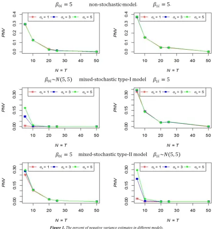
25, and 50. The simulation results are summarized in figures 1 and 2. Specifically, Figure 1 presents the percent of
negative variance (PNV) estimates of Ar. While the results for
the power of Swamy’s test are presented in Figure 2.
Figure 1 indicates that the values of PNV are not appearing
when = ≥ 10 if the parameters are stochastic. However,
if one or more of the parameters is non-stochastic, the values
of PNV are close to zero when = ≥ 50. Moreover, the
values of PNV are increasing when the value of /0 is
increased.
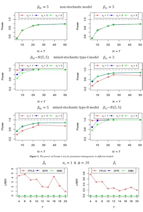
Figure 2 indicates that when the parameters are stochastic
the power of test is very high (close to one) when = ≥
20. However, if one or more of the parameters is
non-stochastic, the power of test is still low even if = ≥ 50.
Moreover, the power of test is increasing when the value of
/0 is decreased.
From figures 1 and 2, conclude that if the sample size ( and/or ) less than 20, the efficiency of stochastic parameter estimators ( PQR̅O , ̅OPQRPS, and ˆŠr•PQRPS) is very affected. Therefore, the efficiency of these estimators in small samples will be examined.
5.2. Second Study: The Performance ofEstimators in Small Samples
In this study, the model in (19) was generated as follows:
1. The values of the independent variable, , were
generated as independent normally distributed random variable with mean 5 and standard deviation 10. The
values of were allowed to differ for each
cross-sectional unit. However, once generated for all N
cross-sectional units the values were held fixed over all Monte Carlo trials.
2. The parameters, 9 and , were generated as in
assumption 4: = 9, = ̅ + @ , where the
vector of ̅ = 5, 5 , and @ were generated as
multivariate normal distributed with mean zero vector and a variance-covariance matrix A∗= D <EFG H; > =
0, 1. The values of G were chosen to be fixed for all >
and equal to 0 or 25. Note that when G = 0, the
parameters are non-stochastic.
3. The errors, , were generated as in assumption
2: = $ , % + & , where the values of & =
& , … , & ∀ = 1, 2, … , were generated as multivariate normal distributed with mean zero vector and a constant variance-covariance matrix /0^ for all . The values of /0and $ were chosen to be: /0 equal
to 1 or 10, and $ equal to 0.35 or 0.95. The initial
values of are generated as
= & ¹1 − $ ⁄ ∀ = 1, 2, … , . The errors were allowed to differ for each cross-sectional unit on a given Monte Carlo trial and were allowed to differ between trials. The errors are independent with all independent variable.
4. The values of = 5 and were chosen to be 4, 6, ..., or 20 to represent small samples for the number of the cross-sectional units and time dimension.
5. The number of replications (¶) is 5000 for each
experiment, and all the results of all separate experiments are obtained by precisely the same series of random numbers.
To compare the small samples performance for the different estimators, the three different types of regression parameters (non-stochastic, stochastic, and mixed-stochastic) have been designed in this simulation study. To raise the efficiency of the comparison between these estimators, the relative efficiency ratio (RER) for each estimator has been calculated. The RER of any estimator, for a Monte Carlo experiment, is calculated by:
RER V ̅O ¼W
= ½.
U<7µ V ̅O ¼W¿½.
U<7µ V ̅O ¾W; > = 0,1
,
where
½. U<7µ V ̅O ÀW =• ∑ U<7•Á µ V ̅O ÀWÁ, for < = 6, Â,
where the subscript 6 indicates the estimator that it calculated the ratio, while  indicates the appropriate estimator in each model in this simulation study. For example, The RER value of FPLS estimate of 9̅ when the all regression parameters are stochastic is calculated as:
Step 1: Calculate the mean of variance for ¶ Monte Carlo trials for FPLS and SPRSC estimators:
½. U<7µ V ̅O9 ÃQ•PW =• ∑ U<7•Á µ V ̅O9 ÃQ•PWÁ,
½. U<7µ V ̅O9 PQRPSW =• ∑ U<7•Á µ V ̅O9 PQRPSWÁ,
where U<7µ V ̅O9 Q•PW and U<7µ V ̅O9 PQRPS W are obtained using feasible formulas for (13) and (4), respectively.
Step 2: Find the RER value: RER V ̅O9 ÃQ•PW =
½. U<7µ V ̅O9 ÃQ•PW ½. U<7¿ µ V ̅O9 PQRPSW
.
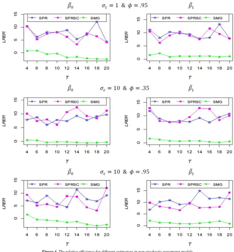
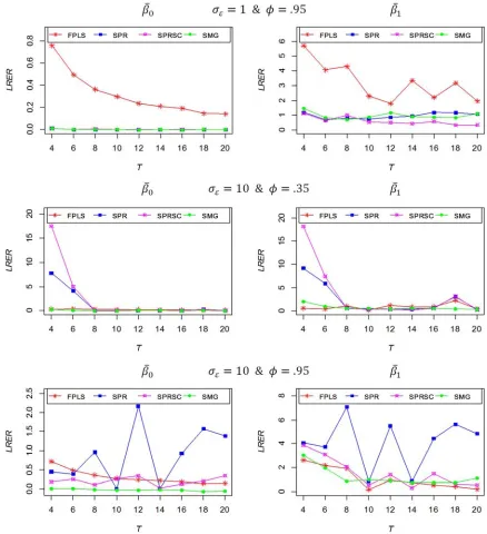
The simulation results are summarized in figures 3 to 6. Specifically, Figure 3 presents the natural logarithm of the RER (LRER) values of intercept and slope estimates for FPLS, SPR, and SMG estimators when the all regression parameters are stochastic (stochastic parameter model). While the results in case of the all regression parameters are
non-stochastic (non-stochastic parameter model) are
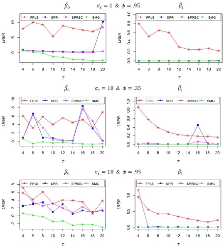
SPRSC, MSPRSC, and SMG estimators when the vector of regression parameters contains both stochastic and non-stochastic parameter (mixed-non-stochastic parameter model). Specifically, Figure 5 displays the results when the intercept parameter is stochastic and the slope parameter is non-stochastic, we refer to this model as Mixed-stochastic type-I
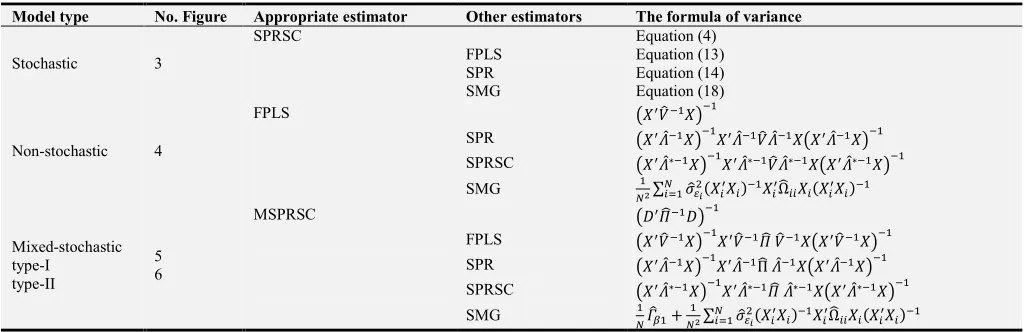
model. Figure 6 displays the inverse case; when the intercept parameter is non-stochastic and the slope parameter is stochastic, also we refer to this model as Mixed-stochastic type-II model. The different formulas of variances of estimators that used in this study are summarized in Table 1.
Table 1. The formulas of variances that used in the simulationstudy.
Model type No. Figure Appropriate estimator Other estimators The formula of variance
Stochastic 3
SPRSC Equation (4)
FPLS Equation (13)
SPR Equation (14)
SMG Equation (18)
Non-stochastic 4
FPLS ) ]r% +%
SPR ) TO% +% TO%]rTO% ) TO% +%
SPRSC ) TO∗% +% TO∗%]rTO∗% ) TO∗% +%
SMG
Ne∑ /yN 01 % Ω€ %
Mixed-stochastic type-I
type-II
5 6
MSPRSC )‡ Ä€% ‡+%
FPLS ) ]r% +% ]r% Ā ]r% ) ]r% +%
SPR ) TO% +% TO%Π€ TO% ) TO% +%
SPRSC ) TO∗% +% TO∗%Ä€ TO∗% ) TO∗% +%
SMG
NAr‰ Ne∑ /y0N 1 % Ω€ %
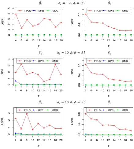
Figure 3 indicates that the values of LRER for SPR and SMG are very close and almost equal zero for all simulation situations (for every value of /0 and $), this means that the efficiency of SPR and SMG is close to the efficiency of
SPRSC estimator even if /0 10 and $ .95, then SPR
and SMG are good alternatives estimators for SPRSC in stochastic parameter models. But FPLS is inefficient estimator (highest LRER) for this model even if /0 1 and
$ .35.
Figure 4 indicates that SPR and SPRSC estimators are
greater in LRER than SMG for every value of /0 and $, this
means that SMG estimator is more efficient than SPR and SPRSC estimators and it is a good alternative estimator for FPLS in non-stochastic parameter models.
Figures 5 and 6 indicate that FPLS is inefficient estimator (highest LRER) for this model for every value of /0 and $. Also, SPR and SPRSC estimators are greater in LRER than SMG in most situations, especially the parameter is non-stochastic. Then SMG estimator is more efficient than SPR and SPRSC estimators and it is a good alternative estimator for MSPRSC in mixed-stochastic parameter models.
6. Conclusion
In this paper, GLS (FPLS, SPR, SPRSC, and MSPRSC) and SMG estimators of panel data models are examined when the errors are first-order serially correlated and the regression parameters are stochastic, non-stochastic, or
mixed-stochastic. Efficiency comparisons for these
Figure 6. The relative efficiency for different estimators in mixed-stochastic parameter type-II models.
Appendix
A. 1 Proof of Lemma 1
a. Show that V ̅OP•´W = ̅:
By substituting O % into (17), it can get:
̅O
P•´ N∑N % N∑N % N∑ ÇN % È. (20)
Taking the expectation for (20) and using assumption 1, it can get:
V ̅OP•´W N∑N ̅.
Under assumption 4: = ̅ + @. By adding
O
to the both sides:O = ̅ + @ + É, (21)
where É = O − = % . From (21), it can get:
N∑N O = ̅ +N∑ @N +N∑ ÉN ,
̅O
P•´ =
Š
+ @Š
+ ÉŠ
, (22)where @̅ =N∑ @N and É̅, =N∑ ÉN . From (22) and using assumptions 1 to 4, it can get:
U<7 VÊ€”½œW = U<7 @̅ + U<7)É̅+ =NA +Ne∑N
/
&2 % Ω % .By using consistent estimators of A,
/
&2, and Ω that defined above, it can get:U<7µ V ̅OP•´W =NAr∗+Ne∑ /yN 01 % Ω€ %
.
(23)
A. 2 Proof of Lemma 2:
Since plim
→¤
% and plim
→¤
% Ω€% are finite and positive definite for all , therefore:
plim →¤ O = plim →¤ O∗= , plim →¤$r = $ , plim →¤
/
t&2 =/
&2, and plim →¤Ω€ = Ω , (24)and then:
plim →¤
/
t&2 ) Ër% +% = plim→¤/
t&2 % Ër % = 0. (25)Using (24) and (25) in (5), it can get:
plim →¤Ar∗=N% V∑N −N∑N ∑N W = A†. (26)
Using (24)-(26) in (23) and (4), it can get:
plim
→¤U<7µ V ̅OP•´W = Nplim→¤Ar ∗+
Ne∑ plimN →¤
/
t&2 % Ër % =NA†, (27)plim
→¤U<7µ V ̅OPQRPSW = plim→¤) Λ€
∗% +% = Y∑ AN †% [% =
NA†. (28)
Similarly, using the results in (24)-(26) in case of SPR estimator:
plim
→¤U<7µ V ̅OPQRW = plim→¤l) Λ€
% +% Λ€% Λ€∗ Λ€% ) Λ€% +% n =
NA†. (29)
From (27)-(29), it concludes that:
plim
→¤U<7µ V ̅OPQRPSW = ÂÍ Î→¤U<7µ V ̅OPQRW = plim→¤U<7µ V ̅OP•´W =NA †.
References
[1] Dielman, T. E. (1983). Pooled cross-sectional and time series data: a survey of current statistical methodology. The American Statistician 37 (2):111-122.
[2] Dielman, T. E. (1989). Pooled Cross-Sectional and Time Series Data Analysis. New York: Marcel Dekker.
[3] Livingston, M., Erickson, K., Mishra, A. (2010). Standard and
Bayesian random coefficient model estimation of US Corn– Soybean farmer risk attitudes. In Ball, V. E., Fanfani, R., Gutierrez, L., eds. The Economic Impact of Public Support to Agriculture. Springer New York.
[5] Swamy, P. A. V. B. (1970). Efficient inference in a random coefficient regression model. Econometrica 38:311-323. [6] Swamy, P. A. V. B. (1973). Criteria, constraints, and
multicollinearity in random coefficient regression model. Annals of Economic and Social Measurement 2 (4):429-450. [7] Swamy, P. A. V. B. (1974). Linear models with random
coefficients. In: Zarembka, P., ed. Frontiers in Econometrics. New York: Academic Press.
[8] Rao, U. G. (1982). A note on the unbiasedness of Swamy's estimator for the random coefficient regression model. Journal of econometrics 18 (3):395-401.
[9] Dielman, T. E. (1992). Misspecification in random coefficient regression models: a Monte Carlo simulation. Statistical Papers 33 (1):241-260.
[10] Dielman, T. E. (1992). Small sample properties of random coefficient regression estimators: A Monte Carlo simulation. Communications in Statistics-Simulation and Computation 21 (1):103-132.
[11] Beck, N., Katz, J. N. (2007). Random coefficient models for time-series–cross-section data: Monte Carlo experiments. Political Analysis 15 (2):182-195.
[12] Youssef, A. H., Abonazel, M. R. (2009). A comparative study for estimation parameters in panel data model. Working paper, No. 49713. University Library of Munich, Germany. [13] Mousa, A., Youssef, A. H., Abonazel, M. R. (2011). A Monte
Carlo study for Swamy’s estimate of random coefficient panel data model. Working paper, No. 49768. University Library of Munich, Germany.
[14] Poi, B. P. (2003). From the help desk: Swamy’s random-coefficients model. The Stata Journal 3 (3):302-308.
[15] Abonazel, M. R. (2009). Some Properties of Random Coefficients Regression Estimators. MSc thesis. Institute of Statistical Studies and Research. Cairo University.
[16] Abonazel, M. R. (2016). Generalized random coefficient estimators of panel data models: Asymptotic and small sample properties. American Journal of Applied Mathematics and Statistics 4 (2): 46-58.
[17] Abonazel, M. R. (2017). Generalized estimators of stationary random-coefficients panel data models: Asymptotic and small sample properties, Revstat Statistical Journal (in press). Available at:
https://www.ine.pt/revstat/pdf/GENERALIZEDESTIMATOR SOFSTATIONARY.pdf
[18] Elhorst, J. P. (2014). Spatial Econometrics: From Cross-Sectional Data to Spatial Panels. Heidelberg, New York, Dordrecht, London: springer.
[19] Anh, V. V., Chelliah, T. (1999). Estimated generalized least squares for random coefficient regression models. Scandinavian journal of statistics 26 (1):31-46.
[20] Murtazashvili, I. and Wooldridge, J. M. (2008). Fixed effects instrumental variables estimation in correlated random coefficient panel data models. Journal of Econometrics 142:539-552.
[21] Hsiao, C., Pesaran, M. H. (2008). Random coefficient models. In: Matyas, L., Sevestre, P., eds. The Econometrics of Panel Data. Vol. 46. Berlin: Springer Berlin Heidelberg.
[22] Boot, J. C., Frankfurter, G. M. (1972). The dynamics of corporate debt management, decision rules, and some empirical evidence. Journal of Financial and Quantitative Analysis 7 (04):1957-1965.
[23] Feige, E. L., Swamy, P. A. V. B. (1974). A random coefficient model of the demand for liquid assets. Journal of Money, Credit and Banking 6 (2):241-252.
[24] Boness, A. J., Frankfurter, G. M. (1977). Evidence of Non-Homogeneity of capital costs within “risk-classes”. The Journal of Finance 32 (3):775-787.
[25] Westerlund, J., Narayan, P. (2015). A random coefficient approach to the predictability of stock returns in panels. Journal of Financial Econometrics 13 (3):605-664.
[26] Srivastava, V. K., Giles, D. E. A. (1987). Seemingly Unrelated Regression Equations Models: Estimation and Inference. New York: Marcel Dekker.
[27] Swamy, P. A. V. B. (1971). Statistical Inference in Random Coefficient Regression Models. New York: Springer-Verlag. [28] Judge, G. G., Griffiths, W. E., Hill, R. C., Lütkepohl, H., Lee,
T. C. (1985). The Theory and Practice of Econometrics, 2nd ed. New York: Wiley.
[29] Hsiao, C. (2014). Analysis of Panel Data. 3rd ed. Cambridge: Cambridge University Press.
[30] Rosenberg, B. (1973). A survey of stochastic parameter regression. Annals of Economic and Social Measurement 2: 381-397.
[31] Pesaran, M.H., Smith, R. (1995). Estimation of long-run relationships from dynamic heterogeneous panels. Journal of Econometrics 68:79-114.
[32] Baltagi, B. H. (2013). Econometric Analysis of Panel Data. 5th ed. Chichester: John Wiley and Sons.
[33] Abonazel, M. R. (2014). Some Estimation Methods for Dynamic Panel Data Models. PhD thesis. Institute of Statistical Studies and Research. Cairo University.
[34] Youssef, A. H., El-sheikh, A. A., Abonazel, M. R. (2014). Improving the efficiency of GMM estimators for dynamic panel models. Far East Journal of Theoretical Statistics 47:171–189.
[35] Youssef, A. H., El-sheikh, A. A., Abonazel, M. R. (2014). New GMM estimators for dynamic panel data models. International Journal of Innovative Research in Science, Engineering and Technology 3:16414–16425.
[36] Youssef, A. H., Abonazel, M. R. (2017). Alternative GMM estimators for first-order autoregressive panel model: an improving efficiency approach. Communications in Statistics-Simulation and Computation 46 (4): 3112–3128.