Information Theory optimization algorithm for efficient service orchestration in distributed systems

(1)

# PREPRINT

# RESEARCH TITLE

Information Theory optimization algorithm for efficient service orchestration

in distributed systems

Matheus Santana Lima Harvard Extension School [email protected]

July 2020, version 0.01

# ABSTRACT

Distributed Systems architectures are becoming the standard computational model for processing and transportation of information, especially for Cloud Computing environments. The increase in demand for application processing and data management from enterprise and end-user workloads continues to move from a single-node client-server architecture to a distributed multitier design where data processing and transmission are segregated. Software development must considerer the orchestration required to provision its core components in order to deploy the services efficiently in many independent, loosely coupled - physically and virtually interconnected - data centers spread geographically, across the globe. This network routing challenge can be modeled as a variation of the Travelling Salesman Problem (TSP). This paper proposes a new optimization algorithm for optimum route selection using Algorithmic Information Theory. The Kelly criterion for a Shannon-Bernoulli process is used to generate a reliable quantitative algorithm to find a near optimal solution tour. The algorithm is then verified by comparing the results with heuristic solutions in 3 test cases. A statistical analysis is designed to measure the significance of the results between the algorithms and the entropy function can be derived from the distribution. The tested results shown an improvement in the solution quality by producing routes with smaller length and time requirements. The quality of the results proves the flexibility of the proposed algorithm for problems with different complexities without relying in nature-inspired models such as Genetic Algorithms and Simulated Annealing. This algorithm can be used by orchestration applications to deploy services across large cluster of nodes by making better decision in the route design.

# Keywords

Traveling Salesman Problem, Information Theory, Artificial Intelligence, Computational Complex Theory, Kolmogorov-Complexity, Kelly criterion and Logarithmic utility

# INTRODUCTION

Distributed Information Systems (DS) are growing in popularity across the software industry as it provides more computational and data transmission capacity for applications and become an essential infrastructure that is needed to address the increase in demand for data processing.

DS are used as a cost-efficient way to obtain higher levels of performance by using a cluster of low-capacity machines instead of a unique – single point of failure - large node. A DS is more tolerant to individual machine failures and provides more reliability than a monolithic system.

(2)

Parallel computation such as Cloud Computing and High-Performance Computing (HPC) are applications of distributed computing. (Marinescu, 2013)

The Cloud Computing market is very consolidated as the cost to deploy, expand and operate a global infrastructure and network is very large. As of 2020 there are 3 major companies: Amazon AWS, Microsoft and Azure. Companies can reduce their IT costs by orchestrating efficiently their workloads across different data centers by their respective weight impact, defined as a utility function with the Euclidian distance between nodes (and its respective influence on network latency) or the financial utilization time-rate cost for a given set of machines. The Figure 1 from Atomia (Alguacil, 2016) illustrate the data centers coverage for the major cloud providers across the globe as of 2016.

Figure 1 A map for the 3 largest Cloud Computing providers by market share of 2016.

The components of a DS are located in many different machines over a network. The communication and orchestration of process are done by sending and receiving messages. The service exposed are defined by the aggregation of components and its interactions provide the software functionality. Systems such as Service-Oriented Architecture (SOA), peer-to-peer(P2P) and Micro-Services are examples of distributed applications.

(3)

There are many algorithms proposed in the literature to solve the routing problem such as 2opt, ant colony, greedy algorithm, genetic algorithm (GA) and simulated annealing (SA) but very limited work is found using Algorithmic Information Theory to find the boundaries of decision problems in Turing Machines. In this paper we propose a variation of the TSP by defining the decision problem for the candidate solution as a Shannon-Bernoulli process that follows a log-normal distribution for the cost distance variable (i.e. created by a utility function for the TSP).

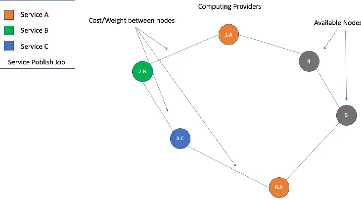
An orchestration job has to deploy efficiently S types of services (or tasks) in many different computing resources such as a cluster of containers or a pool of (physical or virtual) machine nodes connected over a distributed network with different weights (or costs) between each pair of nodes. This job is a process that needs to run on all M (unique) resources points. The cost to use each node can be defined as the (round-trip) network latency between the nodes in the network or the financial cost associated to the proportional quantitative utilization rate for each resource in a given time period. As more Computational Capacity is added, choosing the shortest route to multiple target nodes will be more computationally complex. Figure 2 demonstrate the deployment of services {A, B, C} for nodes {1, 2, 3, 4, 5} in a cluster of machines connected over a common network.

Figure 2 Computing Provider’s distributed over a network of machines with the respective published Service’s and Available nodes

# BACKGROUND

(4)

The Traveling SalesmanProblem was introduced by William Hamilton and Thomas Kirkman. It also known as the messenger problem. The problem asks given a list of cities and the distance between each pair of nodes what is the shortest route that visits all cities exactly once and returns to the original city at the end. There are several researches dedicated to address this routing problem and it has applications in mathematics, computer science, statistics and logistics.

The computational complexity of an algorithm shows how much resources are required to apply an algorithm such as how much time and memory are required by a Turing machine to complete execution and can be interpreted as a measure of difficulty of computing functions. A measurement of computation complexity is the big O notation. It can be defined as: Let two functions f and g such as f(n) is O(g(n)) if there are positive numbers c and N such that

𝑓(𝑛) <= 𝑐𝑔(𝑛) for all 𝑛 >= 𝑁

and is used to estimate the function growth tax (asymptotic complexity).

The TSP problem is an important combinatorial optimization problem. As most of the decision problems, it is in the class of NP-hard problems.

(5)

Figure 3 A sample cost matrix for 4 nodes and the Euclidian distance between each pair of nodes.

Table 1 Solution sample of valid and invalid candidates for a given string schema.

The graph can be represented as a matrix where each cell value is defined as the respective cost (distance) w between nodes v and u. For N nodes the distance matrix is defined as D = w(v,u) for all (unique) pair of N. The goal of the TSP is to find a permutation π that minimizes the distance between nodes. For symmetric instances the distance between two nodes in the graph is the same in each direction, forming an undirected graph. For asymmetric instances the weights for the edges between nodes can be dynamic or non-existent.

The weigh value of the edge is defined as the distance of the tour (roads) between cities.

For symmetric TSP, as the number of nodes (or cities) increases in the graph G, the number of possible tours growth choice also increase and is exponential. If we consider N nodes, the function of the input size is

(6)

This is the number of elements (states) an algorithm must evaluate to decide (to halt) the problem and is very large thus requiring considerable time and computational resources even for small instances of the problem.

A strategy to address this limitation is to accept near-optimal solutions by setting constrains in the problem using heuristics methods (approximations). Algorithms such as 2opt, GA and SA define

𝑎−𝑝𝑟𝑖𝑜𝑟𝑖 knowledge about the distribution of the solution space and then repetitively try to improve the quality. It works by following some heuristic (approximation) function schema while trying to avoid a local minimal. As the heuristics (for TSP and NP problems in general) are a best effort strategy to find a (good) near-optimal solution (by enforcing space and time boundaries), it does not guarantee that the solution found is the best candidate to the problem and therefore an program can never be sure that if by running more time the overall solution cost could be improved, unless the entire solution space to the problem is evaluated. This limitation is set by the definition of NP-hard class.

Computational Complexity Theory Problems in the NP class can be solved by a non-deterministic polynomial algorithm. Any given class of algorithms such as P, NP, coNP, regular etc. must have a lower bound that index the best performance any problem in the class can have. This bound can be described as the total amount of input items (or symbols) a machine must process (before halting), and the respective output items produced following a Probability Distribution Function and a given finite Alphabet. A strategy to find a solution to the decision problem is to find a function that reduce or transform a problem from a domain in which there is no know solution to a constrained domain with a known solution.

This allows the algorithm to search the solution space and decide if any solution is a valid (yes-instances) or invalid (no-(yes-instances) and its computable by a polynomial-time algorithm.

This strategy allows us to map instances of the Hamiltonian circle problem to a decision version of the Traveling Salesman Problem and can be described as a decision problem to determine if exists a Hamiltonian circuit in a given complete graph with positive integer weights hose length is not greater than a given positive integer m. Each valid (yes-instance) in the TSP problem is mapped to a valid instance in the Hamiltonian problem space and this transformation can be done in polynomial time.

(7)

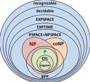
Figure 4 Diagram Representation for the many categories of Computational Complexity

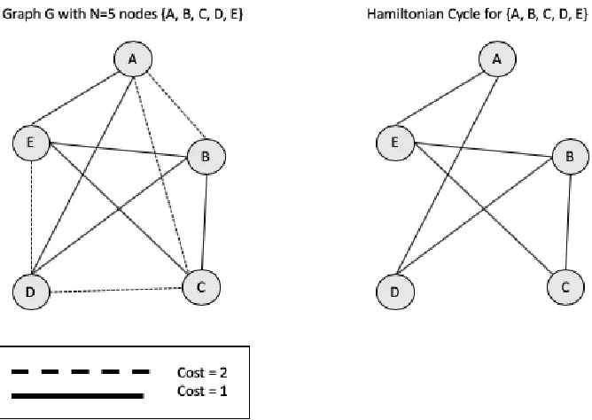
Hamiltonian Graph. A Hamiltonian cycle (or circuit) can described as a "path" that contains all nodes and the elements in this set are not repeated, with exception to the final vertex. This means that a Hamiltonian cycle in G with start node v has all other nodes exactly once and them finishes at node v. A graph G is Hamiltonian if it has a Hamiltonian cycle. A Hamiltonian cycle with minimum weight is an optimal circuit and therefore is the shortest tour in the TSP Problem.

The Figure 5 provides an example of Hamiltonian circuit for a Graph G with 5 nodes {A, B, C, D, E}. The Table 2 shows the cost matrix for the super graph G

Table 2 Cost Matrix for Graph G with 5 nodes

Cost Matrix A B C D E

A 0 2 2 1 1

B 2 0 1 1 1

C 2 1 0 2 1

D 1 1 2 0 2

(8)

Figure 5 Hamiltonian Cycle from a Super Graph

Although heuristics methods define special cases for the TSP problem and produces near-optimal solutions with short length (weight) Hamiltonian cycles it does not guarantee that the results are the shortest circuit possible. The algorithms to solve the TSP are grouped in 2 categories: exact (Brute-force, greedy) and approximation algorithms (Heuristics such as Simulated Annealing and Genetic Algorithm).

Nature inspired models. Researchers have proposed algorithms inspired by natural events and structures like the heating of metals and the growing behavior of biological organisms. Those methods do not iterate over the entire solution space but rather a portion in order to find the local minimum. They start with an initial random solution and tries to improve the solution quality over each interaction until some input Threshold parameter factor T is reached like a maximum number of interactions; maximum number of candidate solutions; no further improvements found after several iterations; the rate of decay in a dependable temperature probabilistic function or a minimum quality threshold is achieved.

Therefore heuristics (approximation) methods can be interpreted as a non-deterministic way to address the error rate between the known solutions and the unknown solutions in polynomial time (i.e. Entropy reduction methods). Although such algorithms do not have to traverse the entire solution space it must decide - or “bet” - when a random candidate solution with negative gain will be accepted (i.e. candidate with worst solution quality than current know best solution) in the hopes that eventually it would lead to the shortest distance (i.e. a better solution quality).

(9)

density function associated with the stochastic process that generates the solutions at random (following a Bernoulli process), thus we can bound the limits of the search space to a log-normal distribution.

The advantage of this method is that by relying on the statistical analysis of the solution space instead of the computational complexity of the problem we can have equal or better quality than the traditional algorithms without relying on computationally complex implementations that have a higher time and space constrains.

Therefore, this paper attempts to provide an algorithm to solve the TSP using for the decision rule the entropy measured for the solution cost distribution H(X) and by maximizing the expected value of the logarithm of cost/weight/distance variable, defined as the utility function g(X). This is equivalent to maximize the expected geometric growth rate.

## CURRENT APPROACH # Literature Review

2opt, k-opt. Croes proposed the 2-opt algorithm (Croes, 1958), a simple local-search heuristic, to solve the optimization problem for the TSP. It works by removing two edges from the tour and reconnects the two paths created. The new path is a valid tour since there is only one way to reconnect the paths. The algorithm continues removing and reconnecting until no further improvements can be found. k-opt implementations are instances of 2-opt function but with k > 2 and can lead to small improvements in solution quality. However, as k increases so does the time to complete execution.

In his work (Glover, 1998) proposed the Tabu Search method and it can be used to improve the performance of several local-search heuristics such as 2opt. As neighborhood searches algorithms like 2opt can sometimes converge to a local optimum, the Tabu search keeps a list of illegal moves to prevent solutions that provide negative gain to be chosen frequently. In 2opt the two edges removed are inserted in the Tabu list. If the same pair of edges are created again by the 2opt move, they are considered Tabu. The pair is kept in the list until its pruned or it improves the best tour. However, using Tabu searches increases computational complexity to O(n3), as additional computation is required to insert and evaluate the elements in the list.

The Figure 6 show the 2-opt moves from (Emir Zunic, 2017).

Figure 6 Generating 2-opt moves

(10)

Tour Improvement algorithms. All algorithms in the first group stops when a solution is found such as brute-force and Greedy Algorithm. In the second group, after a solution is found by some heuristics, it tries to improve that solution (up to certain computation and/or time constraints) such as implemented by 2opt, Genetic Algorithm and Simulated Annealing. He concluded by showing that the computational time required is proportional to the desired solution quality.

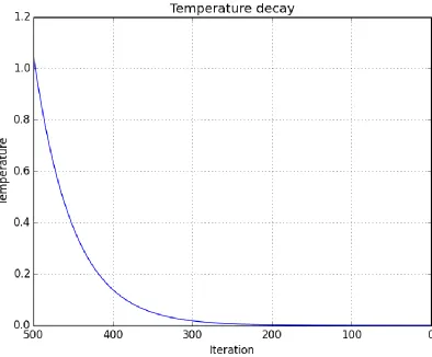
Simulated Annealing (SA). Simulated Annealing are heuristics with explicit rules to avoid local minimal. It can be described as a local random search that temporarily accepts moves with negative gain (i.e. were produced by solutions with worst quality than current). These methods simulate the behavior of the cooling process of metals into a minimum energy crystalline structure.

This concept is analogous to the search of global maximum and minimum. The probability of accepting a solution is set by a probability function of a temperature parameter variable t. As the temperature decreases over time the probability changes accordingly. Figure 7 demonstrates the simulated decay in the temperature function over the number of interactions in an algorithm.

(11)

The acceptance probability is defined as p(x) = 1 if f (y) <= f (x) and when otherwise

p(x) = e^[−(f (y)−f (x))/t] where t is the input temperature.

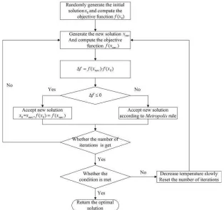
The SA algorithm specifies the neighborhood structure and the cooling function. Figure 8 from (Zhan, 2016)represents the SA algorithm flowchart.

Figure 8 Simulated Annealing Algorithm Flowchart

Metropolis Algorithm. Let f(X) be a function with output proportional to a given target distribution function r. The function r is the proposal density. At each iteration of the algorithm it attempts to move around the sample space. For each move it decides sometimes to accept a given random solution or stay in place. The probability of the solution of the new proposed candidate is with respect to the current know best solution. If the proposed solution is more probable than the know existing point, we automatically accept the new move. Else if the new proposed solution is less probable, we will sometimes reject the move and the more the decrease the probability, more likely we will accept the new move. Most of the values returned will be around the P(X) but eventually solutions with lower probability will be accepted. This characterizes can be interpreted as a generalization of the methods proposed by Simulated Annealing and Genetic Algorithms.

(12)

using a list-based cooling method to dynamically adjust the temperature decreasing rate. This adaptive approach is more robust to changes in the input parameters. In his work (Kah Huo Leong, 2016) proposed a biological inspired bee system to optimize the routing in Railway systems. They conclude that the average solution results are better or equivalent than the traditional SA and GA methods alone.

The quality of the solution can be improved by allowing more time for the algorithm to run. (Steiglitz, 1968) observed that the performance of 2-opt and 3-opt algorithms can be improved by keeping an ordered list of the closest neighbors for each city-node and thus reducing the amount of solutions to search.

Genetic Algorithm (GA). Genetic Algorithms was first introduced by (Holland, 1975) based on natural selection theory, as a stochastic optimization method in random searches for good (near-optimal) solutions. This approach is analogous to the "survival of the fittest" principle presented by Darwin. This means that individuals that are fitter to the environment are more likely to survive and pass their genetic information features to the next generation.

In TSP the chromosome that models a solution is represented by a "path" in the graph between cities. GA has three basic operations: Selection, Crossover and Mutation. In the Selection method the candidate individuals are chosen for the production of the next generation by following some fittest function In the TSP This function can be defined as the length (weight) of the candidate solutions tour. In Figure 9 we have a representation of genes and Chromosomes.

Figure 9 Chromosome for a sample of individual candidate solutions.

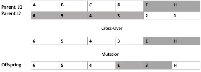
In Figure 10 is demonstrated an example of two parents under the Mutation and Crossover operators to generate a new offspring.

Figure 10 Offspring representation for the Genetic Algorithm Mutation and Crossover operators.

(13)

probability to improve solution in the future. In other words, the heuristic accepts solutions with negative gain hoping that eventually it may lead to a better solution.

Several researches have studied the performance trade off of selection strategy and how the input parameters affect the quality of solution and the computational time. (Razali, 2011) in his work explores different selection strategies to solve the TSP and compare the performances quality and the number of generations required. It concludes that tournament selection is more appropriate for small instance problems and rank-based roulette wheel can be used to solve large size problems.

(Goldberg, 1991) compared the quality of the solution and the convergence time on many selection methods such as proportional, tournament and ranking. They conclude that ranking and tournament have produced better results that proportional selection, under certain conditions to convergence. In his work (Zhong, 2005) explored proportional roulette wheel and tournament method. He concluded tournament selection is more efficient than proportional roulette selection.

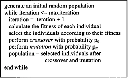
The Figure 11 contains the pseudo-code for a Genetic Algorithm from (K.P. Ferentinos, 2002)

Figure 11 Basic genetic algorithm.

## ALTERNATIVE APPROACH

Information Theory (IT) quantifies the amount of information in a noisy communication channel and is measured in bits of entropy. IT is based in probability theory and statistical distributions. Entropy quantifies the amount of uncertainty in a random Bernoulli variable created by a Bernoulli process thus information can be interpreted as a reduction in the overall uncertainty about a set of finite states. Mutual information is a measure of common information between two random variables and it can be used to maximize the amount of information shared between encoded (sent) and decoded (received) signals. In Table 3 we have the relationship between Information and Entropy. As we increase our knowledge about the states following a probabilistic function distribution, we reduce entropy, as there is less uncertainty about possible state outcomes.

Table 3 Relation between the level of uncertainty and knowledge about possible string outcomes

(14)

High Low 0000 1 0 1*1*1*1 = 1 Medium Medium 0001 0.75 0.25 0.75*0.75*0.75*0.25 = 0.105

Low High 0011 0.5 0.5 0.5*0.5*0.5*0.5=0.0625

Information Theory as an approximation method. Information Theory has applications in a range of fields and is used as a mathematical framework for encoding and decoding of information such as in adaptive systems, artificial intelligence, complex systems, network theory, coding theory, etc. IT quantifies the number of bits required to describe a given data using a statistical distribution function for the input data.

Entropy of a random sequence. Entropy is a measure of uncertainty of a random variable. It is the average rate at which information is produced by a stochastic process. (Shannon, 1948) defined the entropy H as a discrete random variable X with possible values as outcomes draw from a probability density function P(X). Figure 12 demonstrate the variation in entropy H(X) vs a Bernoulli distribution. In Equation 1 the entropy function is defined as:

Equation 1 Shannon Entropy Formula

Figure 12 Entropy H(X) vs Probality Pr(X=1)

(15)

As an example if g(X1 = 001 = 1) = c1 and g(X2 = 010 = 2) = c2 are the costs of two routes between a set of nodes in a super-graph G*, we can use this function to determine the arithmetical and logical relationship between them and decide if c1 is worst, better, less, greater or equal to c2. Therefore g(X1) < g(X2). The probability density function pdf(Y) can be used to calculate the entropy of the distribution of the cost values. An exponential utility is a special case used to model when uncertainty (or risks) in the outcome between binary states and in this case the expected utility function is maximized depending on the degree of risk preference.

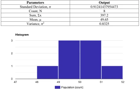
Figure 14 demonstrate an example of a normal distribution for cost function g(X) = {50, 51, 49, 49.3, 50.5, 50.3, 49.1, 48} and the probability P(X<48). Figure 13 shows the histogram for g(X). Table 4 demonstrate the calculation for the mean, standard deviation and variance for g(X), thus we have:

Table 4 Statistical metrics for function g(X) distribution

Parameters Output

Standard Deviation, σ 0.91241437954473

Count, N 8

Sum, Σx 397.2

Mean, μ 49.65

Variance, σ2 _0.8325

(16)

Figure 14 The normal distribution with mean 49.65 and standard deviation 0.91. The P (X<48; X < min g(X)) = 0.0349.

Kolmogorov Complexity. The Kolmogorov complexity (Kolmogorov, 1968) of a string w from language L denoted by Kc_L(w) is the shortest program from alphabet L which produces w as output and halts. The conditional Kolmogorov complexity of string x relative to word w is defined by Kc_L(w|x) and is the length of the shortest program that receives x as input and produces w as output.

Complexity of a string and shortest description length. Let U be a Universal computer (Universal Turing Machine). The Kolmogorov complexity Kc(x) of a string x of a computer U is

Kc (x) = min length(p) When p: U (p) = x

It is the minimum length program p that output variable x and halts. It’s the small possible program. Let C be another computer. If this complexity is general there is a universal computer U that simulates C for any string x by a constant c on computer C. Thus

Kc (x) U <= Kc (x) C + c

Measuring the randomness of a string. Let Kc (x|y): The conditional Kolmogorov complexity of Xn given Y. Consider for example we want to find the binary string with higher complexity between three variables X1(010101010101010), X2(0111011000101110) and Y (01110110001011). In Table 5 we have the representation and minimal encoding using Xn and Y. Therefore, we can see X1 and X2 can be encoded as combinations of Y and thus Kc(X1|Y) > Kc (X2| Y). This relationship is defined as

Kc (X, Y) = Kc(X|Y) + Kc(Y) = Kc(Y|X) + Kc(X)

Table 5 Example of representation of strings X1 and X2 using substring Y.

(17)

Y 01110110001011 Substring

X1 010101010101010 01 (#7 pairs of bits) + 0 (#1 single bit)

X2 011101100010110 Y + 0

In Figure 15 from (Maier, 2014) we can see a comparison between a series of strings and the correspondent automata state machine and the regular expression patterns (i.e. regex).

Figure 15 Examples of representations of a given input string set using regex and an automaton.

The expected value of the Kolmogorov complexity of a random sequence is close to the Shannon entropy. This relationship between complexity and entropy can be described as a stochastic process drawn to a i.i.d on variable X following a probability mass function pdf(x). The symbol x in variable X is defined by a finite alphabet. This expectation is

E(1/n) Kc(X^n|n) => H(X)

Kelly criterion and the uncertainty in random outcomes. The Kelly strategy is a function for optimal size of an allocation in a channel. It calculates the percentage of a resource that should be allocated for a given random process. It was created by John Kelly (Kelly, 1956) to measure signal noise in a network. The bit can be interpreted as the amount of entropy in an expected event with two possible (binary) outcome and even odds. This model maximizes the expectation of the logarithm of total resource value rather than the expected improvement for the utility function from each trial (in each clock unit iteration in a Turing Machine)

(18)

Similarly, the log-normal Salesman’s can improve his strategy in the long run by quantifying the total of available inside information in the channel (or a tape in the Turing machine) and maximizing the expected value of the logarithm of the value function (defined by Traveled Euclidean distance) for each execution clock. Using this approach, he can reduce his uncertainty (entropy H(X)) while optimizing his rate of distance reduction (solution quality improvement) at each execution time.

The Figure 16 demonstrate the Kelly criterion value over the Expected Growth Rate

Figure 16 Maximization of entropy in random events

Kelly uncertainty distribution. Let E(Y) be the expected value of random variable Y, H(Y) be the measured entropy for the pdf(Y) distribution and K*(E(Y),H(Y)) = f* be the maximization of the expected value of the logarithm of the entropy of the utility function Y=g(X) . This fraction is known as the Kelly criterion and can be understood as the level of uncertainty about a given data distribution of the random variable X relative to a probability density function pdf(Y) of a measured respective cost distribution found at the sample. It’s a measurement of the amount of useful encoded information.

The value of f* is a fraction of the cost-value of g(X) on an outcome that occurs with probability p and odds b. Let the probability of finding a value which improves g(X) be p and in this case the resulting improvement is equal to 1 cost-unit plus (1+) the fraction f. The probability of decreasing quality for Y is (1-p). Therefore, the expected value for log variable (E) is differed in Equation 2 as:

(19)

The maximization of the expected value f* is defined by the Kelly criterion formula in Equation 3

Equation 3 Kelly criterion formula

Where f* is the optimal fraction, b is the net odds, p is the probability of improving quality (win) in Y=g(X) and the q is the probability of decreasing (loss) quality q=(1-p).

For example, consider a program with a 60% chance of improving the utility function g(X) thus p=0.6 (win) and q=0.4 (lose). Consider the program has a 1-to-1 odds of finding a sequence which improves g(X) and thus b=1(1 quality-unit increase divided by 1 quality-unit decrease). For these parameters the program has a 20%(f*=0.20) of certainty that the outcomes produce values that improve the expected value of g(X) over many trials.

Consider another sample case for a fair coin with probability of success (winning) P (1) = 0.5(50%) and failure(losing) P (0) = 0.5(50%). Table 6 demonstrate the amount improved (+) and worsen (-) for each scenario:

Table 6 Yield Returns from Bernoulli process P(1) and P(0)

Probability Output Value

Success (1) Gain (True) + 2 units

Failure (0) Lose (False) - 1 unit

The Total Expected Outcome (TEO) is defined by:

TEO = (50% * 2 units) + (50% * 1 unit) = 0.5 units

The Kelly criterion can be calculated alternatively as:

Total Value Allocated (TVA) = Edge/Odds

TVA = TEO/Amount Earned if Success = 0.5 units / 2 units = 25%

Therefore, there are 25% bits of useful information in the noisy channel.

# METHOD

(20)

Tour improvement – heuristics - algorithms such as 2opt and Simulated Annealing (SA) are used as a benchmark for the proposed Quantitative Algorithm (QA). 3 test cases are used to analyses the solutions generated by each algorithm. The 2opt algorithms produces solutions with smaller total distance but required more time units as the number of nodes increase. SA and QA have a maximum number of allowed interactions, but QA produces better solution quality than SA for the same time period.

The test samples are grouped in 10, 30 and 50 nodes. Each point represents a machine in a data center (i.e. computing and network provider) that can deploy a given service S. The distance cost in this case is the illustrative round-trip network and processing delay. This weight is the length of time to send a signal t(s*) plus the time to reply acknowledging of that the same signal t(s*) was received.

To avoid bias and miss interpretation in the research, the first tour loaded in the computer memory is randomly flushed using a statistical function in Python programming language. The function swaps all elements (using a normal distribution) of the initial tour list, created after reading the list of input nodes.

The solutions found from SA and QA heuristics algorithms were analyzed for accuracy and reliability of the output. We have compared the required time and solution improvement between each program. Each algorithm was measured with a trial with sample N=60.

# RESULTS – PROPOSED MODEL

(21)

Figure 17 Flowchart for the Quantitative TSP Algorithm interpretation using Information Theory

Table 7 Proposed algorithm to solve the TSP

Step Procedure Block

0 List of nodes $L[] <= Parse TSP input file Parameter

1 Set maximum number of iterations $max_int Parameter

2 Set s0 as the initial tour created with $L[] Parameter

(22)

Set Probability of Failure P(0)=$q=1-p

4 Set Decay rate value to $decay_rate=0.01(1%) Parameter

5 Set expected cost quality increase E_Q(+Cost)=$e1

Parameter

6 Set expected cost quality decrease E_Q(-Cost)=$e0

Parameter

7 Randomly Flush solution $s0 Parameter

8 Set $first_cost = tourDistance($s0) Parameter

9 Set $min_Tour = $s0 Parameter

10 Set $minCost = tourDistance($s0) Parameter

11 The following steps will be repeted for $max_int times ($i=0; $i<=$max_int)

Main

11 Set $s_new = Create new random solution from $s0

Main

11 if (tourDistance($s_new) < tourDistance($s0)) then

{ if(tourDistance($s_new) < $minCost) then $minCost = tourDistance($s_new); $minTour =

$s_new) }

Main - Decision Module - New shortest solution found

11 elif kelllyCriterion($b) == True then $s0 = $s_new Main - Decision Module - New solution cost is greater than current know solution - Call

Decision Module

11 Calculate the ratio $b = $e1/$e0 Decision Module - Kelly

Criterion Calculate the net-odds 11 Calculate the Kelly fraction $f_k = ($p*($b+1) -

1)/$b

Decision Module - Kelly Criterion

11 Calculate $p = $p - $decay_rate Decision Module - Kelly

Criterion - Decrease Success Probability

11 Pick number $uniformRandom =

random_float(0,1)

Decision Module - Kelly Criterion - Pick random float

number with function

11 Pick number $bernoulli_trial =

Bernoulli_Sequence(Simbols=[0,1], $p_1=0.01, $p_0=0.999)

Decision Module - Kelly Criterion -

Pick random number with weighted distribution. The weigh is the possibility of

each output result. 11 if ($uniformRandom < $f_k or $bernoulli_trial ==

1) then Return True Else Return False

Decision Module - Kelly Criterion

(23)

12 Output the near optimal solution found Halt Execution

Table 8 Overview of the mathematical model with parameters and constraints.

Mathematical Model Category

L : List of nodes Parameter

max_int: Maximum number of iterations (positive) Parameter

s0: Initial tour created with L (path sequence) Parameter

P(1)=p: Probability of Success Parameter

P(0)=1-q: Probability of Failure Parameter

decay_rate: Decay probability rate (for each iteration) Parameter

e1: Expected cost quality increase (total cost reduction) Parameter

e0: Expected cost quality decrease (total cost increase) Parameter

first_cost: Sarting solution cost Parameter

min_Tour: Minimal tour solution Parameter

minCost: Minimal cost Parameter

b: Ratio of quality improvement, b=e1/e2 Parameter

Z: Standard normal variable with u and v > 0 be two real numbers with parameters u and v

Parameter

f* = (p*(b+1) - 1)/b with parameters p=P(1), decay_rate and b Constraint 1 - Kelly Distribution

X = e^(u+(v*Z))

Constraint 2 - Log-Normal Distribution

P(X=1) = p = 1 - P(X=0) = 1-q Constraint 3 -

Bernoulli Distribution

(24)

alternative solution has a negative gain (i.e. new proposed solution is worse than current best-known encoded candidate).

Solutions to the TSP routing problem are explored by algorithms such as 2opt, Simulated Annealing (SA), Greedy and Genetic Algorithm (GA). In this paper we proposed a Quantitative Algorithm (QA) that does not rely on naturally inspired schemas but rather provides a statistical interpretation as a distribution of signals by a stochastic (log normal) process.

This stochastic process is defined as an ordered list of random variables {Xn} for a given trial of length N. N is a set of non-negative integers and Xn is defined as a target measurement for a specific instance of time.

The utility function is used to find the near optimal route that have the minimum traveling distance to multiple target node destination while returning to the starting node at the end. There are 2 constraints to be considered in the model presented in this paper: Simulated Entropy Uncertainty and Bernoulli Process.

## CONSTRAINT 1

Simulated Uncertainty. The first constraint is limited by the entropy. The input parameters for the Kelly function f* are the Wining probability P_W and the expected net-odds b for the Bernoulli trial B. The value of P_W is decreased by a fixed rate of 1% (0.01) at each interaction. The value b is measured as the ratio of average improvements of the positive interactions i+ divided by the average reduction of the negative interactions i-. The result of this function is the percentage of the useful side information available in a noisy channel.

In Table 9 we have an example for the Kelly criterion calculation

Table 9 Example calculation for the Kelly criterion for P (1) = 90, 50 and 10 and net-odds b=1

P (Win/Cost Decrease) P (Lose/Cost Increase) Expected (Averaged) Cost Gain (Quality Improvement) Expected (Averaged) Cost Loss (Quality Worsening) Win/Loss Ratio b (Output) Kelly Percentage f*

90 10 +100 -100 +100/|-100|=1 0.8

50 50 +100 -100 +100/|-100|=1 0

10 90 +100 -100 +100/|-100|=1 -0.8

(25)

Figure 18 Decision Criterion 1 is implemented as the IF statement of the – simulated - Kelly Criterion and the Bernoulli Log-Normal Distribution with output A.

## CONSTRAINT 2

Bernoulli Process. The second constraint is defined by a Bernoulli process as a finite sequence of independent and random Bernoulli variables (i.i.d). This module will return as output the value “True” at 1% of the time for 100 interactions (N=100) and it will accept unlikely (risky) solutions with negative gain to eventually provide improvements bets for the solution quality under some degree of freedom. The process is defined as a trial with two binary states either “True/Success” (1) or “False/Failure” (0) with domain 0 <= p <= 1

P (Xi = 1) = p P (Xi = 0) = 1 – p

E(X) = p

Variance Var (X) = p – pˆ2

In Figure 19 we can see a Bernoulli distribution with P (0) = 80% probability of output a Failure state

(26)

Figure 19 P(X) for the Bernoulli distribution with P(1)=0.2 and P(0) = 1 - P(1) = 0.8

Examples of Bernoulli trials are show in Table 10

Table 10 Examples of random events and the respective binary outcome

Event Outcome

Play a game Win/Lose

Coin toss Head/Tail

Processing a request On time/Late

Defect in equipment’s Good/Defect

Buy-Sell an asset Profit/Deficit

Optimizing traveling cost Reduction/Increase

(27)

Figure 20 Decision Criterion 2 is implemented as a OR gate using for the input (a) Bernoulli Distribution Trial (B) and (b) The IF statement of the – simulated - Kelly Criterion and the Bernoulli Log-Normal Distribution (A).

# DISCUSSION - COMPUTATIONAL RESULTS

The research evaluates the performance of the proposed algorithm through a series of test cases and statistical analysis. The new method is tested against the traditional method Simulated Annealing. Each test case was run for a trial with population size of N=60. In the statistical analysis section, the t-test was used to compare the means between the sample groups. The null hypothesis is that there is no difference between the means of the two populations.

# TEST CASES

The test cases are a set with 20, 30 and 50 nodes. The network latency between each node is bounded by the geographic distances between the machines made available by the computing service provider. The proposed algorithm was used to find the near optimal tour required before returning to the first service endpoint. In Table 11, Table 12, Table 13 we present one sample from the 180 trials to show the comparisons between QA and SA. Each table shows the first initial tour, the optimal solution found, and the time resource required (in seconds) for each algorithm for a sample single execution.

Table 11 Test case with 20 nodes

Node#20 (x, y):

(28)

4 256 141 5 256 157 6 246 157 7 236 169 8 228 169 9 228 161 10 220 169 11 212 169 12 204 169 13 196 169 14 188 169 15 196 161 16 188 145 17 172 145 18 164 145 19 156 145 20 148 145

# Quantitative Algorithm

First solution path: ['1', '20', '8', '7', '17', '13', '2', '3', '16', '9', '15', '11', '14', '10', '6', '19', '4', '5', '18', '12']

Total distance cost from the first(starting) solution: 1145.7617186058662

Best solution Path: ['6', '5', '1', '2', '3', '4', '9', '15', '16', '17', '18', '19', '20', '14', '13', '12', '11', '10', '8', '7']

Total distance cost for the best solution found: 332.1144088148687

Node#30 (x, y):

(29)

12 204 169 13 196 169 14 188 169 15 196 161 16 188 145 17 172 145 18 164 145 19 156 145 20 148 145 21 140 145 22 148 169 23 164 169 24 172 169 25 156 169 26 140 169 27 132 169 28 124 169 29 116 161 30 104 153

# Quantitative Algorithm

First solution path: ['20', '24', '23', '9', '2', '6', '21', '15', '27', '1', '11', '14', '29', '25', '5', '28', '13', '7', '18', '22', '26', '4', '19', '12', '3', '17', '10', '30', '8', '16']

Best solution Path: ['4', '9', '12', '13', '14', '24', '23', '25', '22', '26', '27', '28', '29', '30', '21', '20', '19', '18', '17', '16', '15', '11', '10', '8', '7', '6', '5', '1', '2', '3']

Node#50 (x, y):

(30)

8 228 169 9 228 161 10 220 169 11 212 169 12 204 169 13 196 169 14 188 169 15 196 161 16 188 145 17 172 145 18 164 145 19 156 145 20 148 145 21 140 145 22 148 169 23 164 169 24 172 169 25 156 169 26 140 169 27 132 169 28 124 169 29 116 161 30 104 153 31 104 161 32 104 169 33 90 165 34 80 157 35 64 157 36 64 165 37 56 169 38 56 161 39 56 153 40 56 145 41 56 137 42 56 129 43 56 121 44 40 121 45 40 129 46 40 137 47 40 145 48 40 153 49 40 161 50 40 169

(31)

First solution path: ['38', '48', '39', '40', '9', '26', '28', '29', '33', '43', '41', '14', '12', '23', '1', '17', '20', '5', '49', '7', '35', '22', '18', '31', '6', '19', '13', '36', '2', '16', '42', '15', '4', '32', '25', '46', '8', '47', '50', '27', '37', '24', '34', '3', '10', '30', '45', '21', '44', '11']

Best solution Path: ['49', '48', '47', '41', '42', '43', '44', '45', '46', '40', '39', '38', '37', '36', '35', '34', '33', '32', '31', '30', '29', '21', '20', '19', '18', '17', '16', '9', '5', '1', '2', '3', '4', '6', '7', '8', '10', '11', '12', '15', '13', '14', '24', '23', '25', '22', '26', '27', '28', '50']

(32)

(33)

Table 14, Table 15, Table 16 compares the results between the proposed algorithm and the heurists methods. They demonstrate that the result generated by the QA algorithm achieves solutions with better quality than the SA heuristic algorithm by finding optimal solutions with smaller total cost. The QA algorithm converges more quickly than the 2opt algorithm for large instances of the problem. The results suggest the proposed Quantitative Algorithm is likely to perform better and generate consistent results as other traditional heuristics methods applied to the TSP. Additionally it provides an Information Theory modelling for Computationally Complex domains such as the NP class of problems in Turing Machines.

(34)

Table 14 Difference Scores Calculations for n=10 Nodes and N=60 trials.

t-Test: Two-Sample Assuming Unequal Variances Cost Variable

QA SA

Mean 336.552862 339.645729

Variance 6.35307736 18.1161823

Observations 60 60

Hypothesized Mean Difference 0

df 96

t Stat _-4.8431338

P(T<=t) one-tail _2.4468E-06

t Critical one-tail _1.66088144

P(T<=t) two-tail _4.8935E-06

t Critical two-tail 1.98498431

The result is significant at p < .05.

The 60 iterations who executed the QA algorithm (M = 336.552, Var = 6.353) compared to the 60 iterations in the SA algorithm (M = 339.645, Var = 18.116) demonstrated significantly better cost reduction, with value p = 4.8935E-06.

t-Test: Two-Sample Assuming Unequal Variances Execution Time Variable

QA SA

Mean 28.1821012 34.06591929

Variance 43.5437993 69.06678708

Observations 60 60

df 112

t Stat _-4.2948228

P(T<=t) one-tail _1.8689E-05

P(T<=t) two-tail _3.7379E-05

(35)

(36)

Table 15 Difference Scores Calculations for n=30 Nodes and N=60 trials

t-Test: Two-Sample Assuming Unequal Variances Cost Variable

QA SA

Mean 455.9177842 500.1505

Variance 917.1905283 3396.48698

Observations 60 60

df 89

t Stat

-5.216694386

P(T<=t) one-tail 5.88396E-07

P(T<=t) two-tail 1.17679E-06

The 60 iterations who executed the QA algorithm (M = 455.917, Var = 917.190) compared to the 60 iterations in the SA algorithm (M = 500.150, Var = 3396.486) demonstrated significantly better cost reduction, with value p = 1.17679E-06.

QA SA

Mean 45.3019303 53.1616159

Variance 83.6019137 82.7521257

Observations 60 60

df 118

t Stat _-4.7202404

P(T<=t) one-tail _3.2683E-06

P(T<=t) two-tail _6.5365E-06

(37)

(38)

Table 16 Difference Scores Calculations for n=50 Nodes and N=60 trials.

t-Test: Two-Sample

Assuming Unequal

Variances Cost Variable

QA SA

Mean 901.7845936 960.3116942

Variance 8917.028193 18189.17941

Observations 60 60

Hypothesized Mean

Difference 0

df 106

t Stat -2.753583529

P(T<=t) one-tail 0.003468798

t Critical one-tail 1.659356034

P(T<=t) two-tail 0.006937597

The 60 iterations who executed the QA algorithm (M = 901.784, Var = 8917.028) compared to the 60 iterations in the SA algorithm (M = 960.311, Var = 18189.179) demonstrated significantly better cost reduction, with value p = 0.006937597.

QA SA

Mean 67.6962824 78.4087974

Variance 215.812669 334.607097

Observations 60 60

df 113

t Stat _-3.5368778

P(T<=t) one-tail _0.00029419

P(T<=t) two-tail _0.00058839

(39)

The 60 iterations who executed the QA algorithm (M = 67.696, Var = 215.812) compared to the 60 iterations in the SA algorithm (M = 78.408, Var = 334.607) demonstrated significantly better time to complete execution, with value p = 0.00058839.

These findings can be expanded to other complex problems and it scales linearly to the search space sample. The proposed method is also resistant to the time and space constraints and it has a constant number of maximum iterations. In this paper we have introduced a new interpretation for the entropy rate for a binary program that implements a given NP problem.

The results can be used by many real-world applications such as the optimization of routing messages over a network and the orchestration of services across a distributed system such as provided by Cloud Computing environments and micro-services-oriented architectures. Besides it is also a future reference on the subject of Information Theory, Computational Complex Theory and Logarithmic utility in optimization routing, deployment, scheduling and planning. The research demonstrated that the proposed concepts have statistically significant results with better solution quality in tour planning. The model provides a new interpretation of entropy in problems encoded in Turing Machines and has the potential to change the traditional interpretation of the limits of Computing Theory.

The results are statistically significant (with p-value < 0.05), and we can conclude the proposed algorithm has better solution quality with reduced computational requirements and better cost improvement.

## STATISTICAL CASE STUDY

In order to test the performance in solving the TSP we have created trials with sample size N=60 for each test case with different number of nodes n={10, 30, 50} and then compared the results obtained from a traditional heuristic (SA) and the proposed algorithm (QA).

Table 17 demonstrate the two-tailed t-test for two independent samples of costs with Significance Level of 0.05. This is a two-sided test for the null hypothesis with two independent means have the identical expected value. This test measures if the average expected cost value differs significantly across the measured samples. If the p-value is small than the significance level of 0.05 (5%) then we can reject the null hypothesis of equal average means.

Table 17 Comparison matrix for the two-tailed t-test independent means p-values for the test cases with nodes with n=20, 30, 50 and sample size N=60

20-node 30-node 50-node

Cost variable t-test

for N=60 QA-SA. QA-SA. QA-SA.

p-value 4.89351E-06 1.17679E-06 0.0069376

(40)

Time variable t-test

for N=60 QA-SA. QA-SA. QA-SA.

p-value 3.73787E-05 6.53652E-06 0.00058839

The Table 17 shows that results are statistically significant (with p-value < 0.05) for test cases n={20, 30, 50}, and we can conclude the proposed Quantitative Algorithm (QA) has better solution quality with reduced computational requirements and better cost improvement than heuristic Simulated Annealing (SA).

# CONCLUSION

Service scheduling and network routing has many applications and is related to the optimization problem modeled by the Traveling Salesman Problem. It’s possible to improve performance by reducing the cost of transmission of information across many distributed systems locations. A new interpretation and verified optimization algorithm and statistical model based in Information Theory is presented in this paper and it demonstrated how it can be used to solve the TSP. The results support the idea that the proposed method can be used reliably to generate solution under a given degree of freedom. The algorithm can be expanded to large scale problems without the high requirements of computational resources utilization imposed by the brute-force and traditional heuristics methods such as Simulated Annealing and Genetic Algorithms. The algorithm can be adapted to any case of the routing problem. The research can be used as a framework for future works and extend the implications of Information Theory and Kolmogorov-Complexity in solving TSP and NP Problems in general.

The advantage of this approach is that it is independent of the computer encoding the problem and the time and space complexities are additive up to a limit that is linearly proportional to the input size. Other heuristics methods assume a predefined knowledge about the data structure and thus are biased towards this encoded schema. The implications of this interpretation is that by reducing the NP problems to a matter of modularization of encoded and decoded random signals in an communication noisy channel, we can find near optimal solutions that are statistically significant and are guaranteed to produce the best rate of improvement in the long run over many trials(i.e. simulation iterations) even though the problems itself is computationally complex and the alternative sequential brute force algorithm would require exponential time to solve. This mathematical model can be interpreted as a generalization of heuristics methods.

The findings in this paper unifies critical areas in Computing Science, Mathematics and Statistics that many researchers have not explored and provided a new interpretation that advances the understanding of the role of entropy in decision problems encoded in Turing Machines.

# REFERENCES

Bibliography

(41)

Cover, T. M. (2012). Elements of information theory. John Wiley Sons.

Croes, G. A. (1958). A method for solving traveling salesman problems. Operations Research. Deb., D. E. (1991). A Comparative Analysis of Selection Schemes Used in Genetic Algorithms.

Proceedings of the World Congress on Engineering. Vol II .

E. H. Aarts, J. H. (1988). A quantitative analysis of the simulated annealing algorithm: a case study for the traveling salesman problem. Journal of Statistical Physics.

Emir Zunic, A. B. (2017). Design of Optimization System for Warehouse Order Picking in Real Environment. XXVI International Conference on Information, Communication and Automation Technologies (ICAT).

Glover, L. M. (1998). Tabu Search. Handbook of Combinatorial Optimization. Springer: Boston, MA .

Goldberg, D. E. (1991). A comparative analysis of selection schemes used in genetic algorithms. Foundations of genetic algorithms: Elsevier.

Hasegawa, M. (2011). Verification and rectification of the physical analogy of simulated annealing for the solution of the traveling salesman problem. . Physical Review E, vol. 83.

Holland, J. H. (1975). Adaptation In Natural And Artificial Systems. University of Michigan Press. Jinghui Zhong, X. H. (2005). Comparison of Performance between Different Selection Strategies on Simple Genetic Algorithms. Proceedings of the World Congress on Engineering. Vol II.

K.P. Ferentinos, K. A. (2002). Heuristic optimization methods for motion planning of autonomous agricultural vehicles. Journal of Global Optimization.

Kah Huo Leong, H. A.-R.-C. (2016). Bee Inspired Novel Optimization Algorithm and Mathematical Model for Effective and Efficient Route Planning in Railway System. Kelly, J. (1956). A new interpretation of information rate. Bell System Technical Journal.

Kim, S. J. (1991). Fast parallel simulated annealing for traveling salesman problem on SIMD machines with linear interconnections. Elsevier Parallel Computing.

Kolmogorov, A. N. (1968). Logical basis for information theory and probability theory. IEEE Trans. Inf. Theory.

Maier, A. (2014). Identification of Timed Behavior Models for Diagnosis in Production Systems. Faculty of Electrical Engineering, Computer Science and Mathematics University of Paderborn.

Marinescu, D. C. (2013). Cloud computing: theory and practice. Morgan Kaufmann. Nilsson, C. (2003). Heuristics for the Traveling Salesman Problem. Linköping University.

Raskhodnikova, S. (2016). CMPSC 464: Introduction to the Theory of Computation Spring 2016.

Retrieved from The Pennsylvania State University :

http://www.cse.psu.edu/~sxr48/cmpsc464/

Razali, N. &. (2011). Genetic Algorithm Performance with Different Selection Strategies in Solving TSP. International Conference of Computational Intelligence and Intelligent Systems (ICCIIS'11).

Sandor P. Fekete, H. M. (2002). Solving a Hard problem to approximate an Easy one: heuristics for maximum matchings and maximum traveling salesman problems. Journal of Experimental Algorithms,.

Shannon, C. E. (1948). A mathematical theory of communication. Bell Labs Technical Journal. Shi-hua Zhan, S. L.-j. (2016). List-Based Simulated Annealing Algorithm for Traveling Salesman

(42)

Steiglitz, K. &. (1968). Some Improved Algorithms for Computer Solution of the Traveling Salesman Problem.

Thorp, E. O. (1997). The Kelly Criterion in Blackjack Sports Betting, and the Stock Market. The 10th International Conference on Gambling and Risk Taking, Montreal, June 1997, published in: Finding the Edge: Mathematical Analysis of Casino Games.

Yang., P. T. (1993). An improved simulated annealing algorithm with genetic characteristics and the traveling salesman problem. Journal of Information and Optimization Sciences.

Zhan, S.-h.-j. (2016). List-Based Simulated Annealing Algorithm for Traveling Salesman Problem. Information.

Zhong, J. H. (2005). Comparison of performance between different selection strategies on simple genetic algorithms. International conference on computational intelligence for modelling, control and automation and international conference on intelligent agents, web technologies and internet commerce (CIMCA-IAWTIC'06) , Vol. 2, pp. 1115-1121. Zhou, A.-H. &.-P. (2018). Traveling-Salesman-Problem Algorithm Based on Simulated

Annealing and Gene-Expression Programming. Information. 10. 7. 10.3390/info10010007. Zhou, A.-H. &.-P. (2019). Traveling-Salesman-Problem Algorithm Based on Simulated

Annealing and Gene-Expression Programming. MDPI Information.

(Alguacil, 2016) (Glover, 1998)

(Raskhodnikova, 2016) (Emir Zunic, 2017) (Jinghui Zhong, 2005) (Shi-hua Zhan, 2016) (Yang., 1993)

(Thorp, 1997) (Shannon, 1948) (Nilsson, 2003) (Razali, 2011)

(Sandor P. Fekete, 2002) (Kolmogorov, 1968) (Kelly, 1956)

(Kim, 1991) (Hasegawa, 2011) (Holland, 1975)

(K.P. Ferentinos, 2002) (Deb., 1991)

(Croes, 1958) (Cover, 2012) (E. H. Aarts, 1988) (Zhan, 2016) (Maier, 2014)

(43)

Table 18 Execution Results for 20 nodes (n=20) with samples size N=60

20-node

Trial N=60 Initial Random Tour Cost Best Tour Cost Found Total Execution Time

0 QA SA QA SA QA SA

1 1195.634925 1108.393775 336.620892 339.439482 30.12948538 39.6077362

2 986.9352715 1177.732299 338.5615264 344.758321 30.26399596 32.3809037

3 900.0458995 1054.1641 334.8573413 345.966652 34.91276873 38.7632731

4 916.5463351 1057.927051 335.3011739 341.855037 27.23480984 38.4763941

5 966.1553232 1253.494224 336.620892 332.114409 29.91621914 32.1631082

6 1194.232179 1064.387485 335.8914965 338.044106 31.12498264 33.1915936

7 1036.191977 1029.253756 338.5615264 340.135251 31.81935215 32.060559

8 963.2410995 999.9887981 339.3638244 339.439482 54.49795967 65.4112282

9 1145.761719 1050.78347 332.1144088 340.059594 25.79352437 50.170809

10 1085.090655 1073.381069 337.2219503 337.316661 27.91745513 35.5128518

11 1147.417441 1012.068389 343.0294931 334.857341 25.94175636 31.4301689

12 965.8459042 958.2459652 334.8573413 335.301174 24.29773869 28.3900081

13 1128.489942 1283.781151 335.9022323 339.231552 29.54066219 37.4386245

14 1131.818667 928.6586146 337.0140207 335.902232 47.45874454 40.282868

15 1229.658241 1153.404679 335.9022323 346.41498 40.86180719 40.4422965

16 884.1357153 1138.13307 332.7154672 338.561526 34.48849958 49.9608527

17 1235.918025 1052.377384 335.9022323 336.620892 28.82108637 37.7635394

18 783.6900544 929.1934876 335.8914965 338.561526 31.23878077 42.0187519

19 1130.320419 1174.181378 337.0140207 342.439171 30.00009195 34.7658014

20 989.3865301 951.2563694 343.5134562 339.363824 35.36053606 40.5407622

21 904.2377617 1063.30281 335.9022323 338.741826 29.65111817 38.7390394

22 869.7243065 1029.595623 335.3011739 338.561526 28.38350387 32.86863

23 1116.176649 953.0821731 334.8573413 338.561526 31.87757207 36.2553472

24 1110.200886 931.6046509 337.3166611 345.685585 43.94790548 40.1406831

25 1064.184077 1139.258709 334.8573413 338.119763 41.20329418 45.7096829

26 887.1252702 940.9695223 335.3011739 345.685585 25.25219875 45.1240136

27 1040.447342 1308.425282 336.4925548 336.620892 23.90627663 28.4887706

28 1263.036989 1297.030551 337.2219503 339.231552 26.12993897 31.0484482

29 1115.022094 1055.582523 337.0140207 335.902232 29.95108272 58.9338429

30 998.9318306 981.3689839 335.9022323 348.044562 35.33063453 44.3207047

31 1127.712215 1066.313009 336.4129623 339.342884 28.56060964 43.9690071

32 945.3399049 1133.277072 335.3011739 338.561526 25.08187038 34.241621

33 1079.60359 913.4123438 338.0441064 334.857341 23.84379763 28.6076721

34 913.3758632 1151.462443 332.1144088 334.932998 24.00100185 28.4874175

(44)

36 1147.723302 1130.778705 338.0441064 343.649497 23.43391117 27.3482798

37 971.3903556 1076.686391 336.620892 332.715467 23.04826988 27.2579731

38 998.2103312 887.1398159 332.1144088 339.439482 23.30005102 27.9801567

39 1162.280089 924.1853956 337.9177195 335.301174 23.55994665 28.0173068

40 1054.008142 869.5783019 345.095262 348.044562 24.4069206 28.0580326

41 1062.958346 1092.610068 337.3166611 334.857341 23.58406409 30.9849236

42 1316.550471 1132.915517 335.9022323 332.715467 24.49907442 27.7148466

43 944.5629418 1096.900034 334.8573413 338.561526 27.42394148 29.689707

44 1090.841136 973.9952212 336.620892 345.879822 23.22344759 30.1561858

45 985.9883167 915.8312807 338.0441064 343.428117 23.68698814 27.5134631

46 1193.337578 1001.967642 332.7154672 337.22195 23.15058773 27.6503922

47 1085.046538 1056.207841 336.4129623 339.439482 22.89809065 27.6979532

48 1170.592904 1204.896611 332.7154672 335.301174 22.811833 27.1470865

49 888.3716219 1119.310235 332.7154672 353.222205 23.53460078 27.1795784

50 957.744169 896.1779984 339.4394815 337.917719 22.97475352 27.4758247

51 1105.010107 1023.615603 338.0441064 338.710086 22.86918458 27.2797519

52 868.7296417 1001.961386 336.4925548 341.484758 23.09712953 27.1193013

53 1147.110698 1261.361139 336.620892 338.561526 23.20182619 27.8441451

54 1007.496906 1076.417337 336.4129623 339.231552 22.91703718 27.7154546

55 888.3254017 1028.532428 334.8573413 337.014021 23.08894057 27.652091

56 1015.389387 1037.982865 338.5615264 335.301174 24.19610564 27.4061656

57 1118.083211 1218.690552 334.8573413 343.500897 23.50864635 27.9921575

58 1196.871246 1056.936272 334.8573413 343.428117 23.84533973 27.6875045

59 1172.5209 765.331396 339.3638244 340.059594 23.19705539 27.9977026

60 1225.40291 1041.148332 339.3638244 345.962516 32.50677825 27.3577434

Table 19 Execution Results for 30 nodes (n=30) with samples size N=60

30-node

Trial N=60 Initial Random Tour Cost Best Tour Cost Found Total Execution Time

0 QA SA QA SA QA SA

1 2114.861664 2138.958342 424.5873682 464.700899 42.98706438 59.0712779

2 1941.575116 2007.049171 475.6796776 472.590934 39.46565883 52.120306

3 1950.142483 1989.063029 488.989852 504.453757 38.60825704 47.8920127

4 1902.474244 1796.927917 424.3794386 506.801158 48.13539106 61.4913984

5 1580.54924 2121.678062 510.318469 472.980497 44.92054756 44.2866884

6 2040.501524 1887.043741 474.6886065 433.933129 43.33821167 48.5092938

7 1933.189429 2005.284134 426.0105826 478.033092 43.31067901 54.8387858

8 1791.060214 2174.057473 429.9694289 462.536112 40.27118746 50.435126

(45)

10 2159.279821 2101.511052 439.9631361 526.162767 43.91304872 51.6482356

11 2037.032939 1964.471053 436.517103 507.74012 37.68801916 48.1148758

12 2057.901751 1892.015046 467.0236214 562.704654 52.46498072 51.1041011

13 1930.750408 1831.163179 460.014352 426.528003 52.34054281 79.7551805

14 1596.34284 1709.164989 484.0191023 571.764133 41.91429676 57.815061

15 1989.991866 1932.746628 453.6891305 428.101727 52.06071529 63.1093559

16 1532.819374 2294.07567 432.8197583 443.083125 45.44243764 61.380042

17 1933.611183 2091.996596 453.529067 595.347046 40.35533853 50.0510586

18 1928.551184 1860.347264 495.9653506 580.368162 43.90844072 46.7043453

19 1892.952203 2098.647235 491.0938606 468.450763 45.20533055 53.5513851

20 1727.389612 1746.213002 428.8730412 587.027872 39.56974309 50.744991

21 1840.460231 2052.640373 486.8539675 510.278944 55.44163731 51.324384

22 1734.505095 1843.716782 491.0156727 427.122371 40.87608984 57.7772876

23 1804.725607 1840.418372 447.2951117 486.01134 57.19451948 55.1076989

24 1900.969989 1597.14205 460.1507211 662.168972 47.51163171 69.8538226

25 1902.159287 1982.433073 433.0617383 477.980165 52.9507134 52.5828033

26 1861.379571 1732.215165 478.1275476 481.88559 63.18074776 61.506958

27 1632.125705 1705.527663 551.6573018 534.398358 45.71926259 59.901718

28 1724.804881 2004.34791 464.0476771 533.121258 45.68037277 57.0611448

29 1711.276107 1851.488894 426.6765623 565.016049 43.55173205 53.7347876

30 1798.24361 2147.552334 467.8403795 491.540871 39.89643796 48.881184

31 1505.540858 2286.236266 427.122371 592.196033 48.98996233 48.1386252

32 1868.889925 1772.226931 427.4357473 488.765595 47.68942928 50.6868412

33 1986.199157 1831.914237 423.8687085 530.861945 54.60683943 70.0300942

34 1893.774487 2191.409802 476.6245181 482.210099 56.77093291 69.9386231

35 2254.034678 2057.794281 450.6222049 470.823818 50.39574996 56.2931122

36 1641.972013 1951.754928 456.9229002 470.823818 57.52063273 67.2678736

37 2190.641527 1892.120281 427.1980282 479.691631 45.58968535 54.0853191

38 2059.180754 1991.897847 446.6225652 443.410875 43.33406437 68.1481031

39 1816.734006 1938.160932 423.2676502 457.649743 43.01746808 48.3186617

40 2009.362159 2057.941367 442.9039608 449.980838 42.63856604 48.0714487

41 1619.209653 1977.29523 430.5704872 625.975132 63.20465673 72.4023792

42 1803.072488 2008.969722 436.3291255 434.210099 38.81750628 49.0113726

43 1905.327122 2139.748939 431.6159736 422.823818 90.17018865 57.4507498

44 1396.063861 1510.800171 427.122371 446.937846 46.57496965 56.7508254

45 1961.970303 2085.66334 461.2238488 423.868709 40.88945298 47.0390539

46 2016.906558 1945.01613 431.6159736 482.392057 37.00943786 41.2652409

47 1615.747074 1679.767432 438.5243978 540.930956 34.94234454 41.9965412