Formal Specification and Verification of Real-Time Systems using Graph Grammars

(1)

Veriﬁcation of Real-Time Systems

using Graph Grammars

Leonardo Michelon

1

, Simone André da Costa

1,2

and Leila Ribeiro

1

1_{Instituto de Informática}

Universidade Federal do Rio Grande do Sul Av. Bento Gonï£¡alves, 9500 91501-970 - Porto Alegre - RS - BRAZIL

{lmichelon, scosta, leila }@inf.ufrgs.br 2_{Departamento de Informática} Universidade Federal de Pelotas

Campus Universitario, s/n 96010-900 - Pelotas - RS - BRAZIL

{simone.costa }@ufpel.edu.br

Abstract

The importance of real-time systems has enormously increased in the last decade. Application areas that typi-cally need real-time models include railroad systems, in-telligent vehicle highway systems, avionics, multimedia and telephony. To assure that such systems are correct, additionally to prove that they provide the required func-tionality, time constraints must be satisfied. There are al-ready formal specification methods for real-time systems, but most of them are difficult to use by software devel-opers, that are usually not very familiar with mathemat-ical notation but rather specify systems using the object-oriented paradigm. In this paper we propose a formal approach to specify and analyze real-time systems that has an object-oriented flavor. This approach is based on Object-Based Graph Grammars (OBGGs), a formal de-scription technique suitable for the specification of asyn-chronous distributed systems, and intuitive even for non-theoreticians. We extend OBGGs to enable explicit mod-eling of time constraints, and define the semantics of the specifications via transition systems. Finally, we translate timed OBGGs to Timed Automata, a formal notation that is wide spread in the area of real-time systems modeling and allows the automatic verification of properties.

Keywords: Real-time computing, Formal specifica-tion and verificaspecifica-tion, Graph grammars, Timed automata.

1. I

NTRODUCTION

One of the goals of software engineering is to aid the development of correct and reliable software systems. Formal speciﬁcation methods play an important role in accomplishing this goal [7]. Besides providing means to prove that a system satisﬁes the required properties, formal methods contribute to its understanding, revealing ambiguities, inconsistencies and incompletions that could hardly be detected otherwise.

The use of a formal speciﬁcation method is even more important in the design of real-time systems, frequently used in critical security environments. A real-time system is a system in which performance depends not only on the correctness of single actions, but also on the time at which actions are executed [27, 26]. Application areas that typ-ically need real-time models include railroad systems, in-telligent vehicle highway systems, avionics, multimedia and telephony. To assure that such systems are correct, additionally to prove that they provide the required func-tionality, we have to prove that the time constraints are satisﬁed.

1.1. FORMALSPECIFICATION OFREAL-TIMESYS

-TEMS

(2)

prominent methods for real-time speciﬁcation. A timed automaton extends a usual automaton by adding several clocks to states and time restrictions to transitions (and states). It enables us to specify both the discrete behavior of control and the continuous behavior of time. Process calculi models including time [21, 2, 6] have also been proposed, adding a set of timing operators to process alge-bras. They offer a level of abstraction based on processes: a system is viewed as a composition of (interacting) pro-cesses. Timed Petri nets [28] and time Petri nets [5] are extensions of the classical Petri nets adding time values to transitions/tokens or time intervals to transitions, respec-tively.

Although the models discussed above may be ade-quate for some aspects of a system, they stress the rep-resentation of the control structure, lacking a comprehen-sive representation of data structure and its distribution within a system. Object-oriented models provide such abstraction by joining descriptions of data and processes within one object. Distribution and concurrency ap-pear naturally by viewing objects as autonomous entities. Object-oriented approaches are widely accepted for spec-ification and programming. Thus, various Unified Mod-eling Language (UML)-based approaches have already been proposed to model time information. HUGO/RT [18] is an automated tool that checks if a UML state ma-chine interacts according to the scenarios specified by a sequence diagram (extended with time constraints). For this verification, state machines are compiled into Timed Automata and sequence diagrams into Observer Timed Automaton. After the translations, the model-checker Up-paal [3] is called to check if the Observer Timed Automa-ton describes a reachable behavior of the system. Di-ethers and Hunh [9] propose a similar approach through the Vooduu tool. Nevertheless, these tools restrict the specification of a real-time system. First of all, because they are based on UML state machines and therefore do not offer clocks or priorities, useful concepts for real-time modeling. Besides, even though the proposals intent to be faithful to the UML informal specification, following its semantic requirements, the translation of state machines is not based on a formal semantic. In [20] a transla-tion of timed state machines into a real-time specificatransla-tion language TRIO was proposed, but TRIO is not directly model checkable.

The approach in [19] adds time information to UML classes. Attributes of type Timer, for the deﬁnition of clocks for classes, and a notation similar to timed au-tomata, to analyze and evaluate clocks in UML state diagrams, are syntactically introduced. A translation from UML into Promela, the input language of the SPIN model-checker, is extended to give semantics to the dia-grams. The main difﬁculty in using this approach is that, since Promela does not have built-in time constructors,

clocks and time constrains have to be encoded and, since the semantics is deﬁned by the Promela code, it might be quite difﬁcult to understand for users not very familiar with this language.

The Omega project also aims to model and verify real-time systems. An extension of a UML subset with real-time constructs was proposed in [16], and in [22] part of UML was mapped into Communication Extended Timed Au-tomata (input language for the validation tool). Static properties are described as Observer Automata and dy-namic properties by UML Observers. This is a very inter-esting approach, although the user has to learn a variety of different languages and diagrams to completely specify and verify a system.

1.2. OURCONTRIBUTION

In this paper, we propose extending the formal description technique Object-Based Graph Grammars (OBGGs) [11, 23] to specify real-time systems. OBGG is a visual formal specification language suitable for the specification of asynchronous distributed systems. The basic idea of this formalism is to model the states of a system as graphs and describe the possible state changes as rules (where the left- and right-hand sides are graphs). The behavior of the system is described via applications of these rules to graphs modeling the actual states of a sys-tem. Rules operate locally on the state-graph, and there-fore it is possible that many rules are applied at the same time. OBGGs are appealing as specification formalism because they are formal, they are based on simple but powerful concepts to describe behavior, and they have a nice graphical layout that helps non-theoreticians under-stand an object-based graph grammar specification. Due to the declarative style (using rules), concurrency arises naturally in a specification: if rules do not conflict (do not try to update the same portion of the state), they may be applied in parallel (the specifier does not have to say explicitly which rules shall occur concurrently).

OBGGs can be analyzed through simulation [12] and verification (using the SPIN model-checker) [10]. Com-positional verification (using an assume-guarantee ap-proach) is also provided [24]. Moreover, there is an ex-tension of OBGGs to model inheritance and polymor-phism [15]. However, OBGGs do not provide explicit time constructs, and therefore are not suited to model and analyze real-time systems. Here we propose a mapping from a timed extension of OBGG specifications to Timed Automata. This way, we can use the available (Timed Automata) verification tools to check properties of timed OBGGs.

(3)

temporal logic. The main contributions of this paper are: (i) the proposal of a timed extension to OBGG; and (ii) the translation of the extended OBGG to Timed Automata, leading to automatic veriﬁcation of properties. The paper is organized as follows: Section 2 presents OBGGs and its timed extension; Section 3 describes the semantics of timed OBGGs; Section 4 reviews Timed Automata; the translation of timed OBGGs to Timed Automata is de-scribed in Section 5; Section 6 analyzes the example; and ﬁnal remarks are in Section 7.

2. O

BJECT

B

ASED

G

RAPH

G

RAMMARS Object based graph grammar (OBGG) is a formal vi-sual language suited to the specification of object-based systems. We consider object-based systems with the fol-lowing characteristics: (i) a system is composed of var-ious objects. The state of each object is defined by its attributes, which may be pre-defined values or refer-ences to other objects. An object cannot read or mod-ify the attributes of other objects; (ii) objects are in-stances of classes. Each class includes the specification of its attributes and of its behavior; (iii) objects are au-tonomous entities that communicate asynchronously via message passing. An OBGG specifies a system in terms of states and changes of states, where states are described by graphs and changes of states are described by rules.

Now, the definitions used for the description of Timed Object-Based Graph Grammars (TOBGGs) are pre-sented. Each formal definition is preceded by an informal description of its meaning. The formal definitions are necessary to follow the translation of TOBGG to Timed Automata, described in Section 5. For the comprehension of the other contributions of this paper, it is possible to skip the formal definitions. Examples of main concepts can be found in Subsection 2.2.

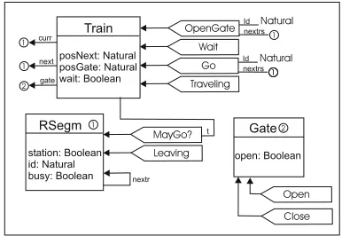
Graph, Graph Morphism. A graph consists of a set of vertices partitioned into two subsets, of objects and values (of abstract data types), and a set of edges partitioned into sets of message and attribute edges. Values are allowed as object attributes and/or message parameters. Messages, modeled as (hyper)edges, may also have other objects as parameters and must have a single target object. These connections are expressed by total functions assigning to each edge its source and target vertices. Figure 1 illustrates a graph for an object-based system. Values of abstract data type Natural are allowed, for example, as attributes of theTrainobject and as parameters of theOpenGatemessage. TheTrain object also has references toGateandRSegm objects as attributes. MessageOpenGate has theTrainobject as target and as sources a reference toRSgmobject and

Train

posNext: Natural posGate: Natural wait: Boolean

nextrs Id Natural

1 OpenGate

nextrs Id Natural

1 Go Wait

Traveling

curr

next gate

1

2

1

RSegm

station: Boolean id: Natural busy: Boolean

Gate

open: Boolean

1 ₂

MayGo? Leaving

t

Open

nextr

Close

Figure 1. Type Graph

Natural values. Agraph morphismexpresses a structural compatibility between graphs: if an edge is mapped, the corresponding vertices, if mapped, must have the same sources/target vertex; if a vertex is mapped, the attributes must be the same.

Letf : A → B be a partial function and let f• be the corresponding total function f• : dom(f) → B, s.t, f(x) = f•(x), ∀x ∈ dom(f). LetSpec be an al-gebraic speciﬁcation, including sort N at and the usual operations and equations for natural numbers, and U :

Alg(Spec)→ Setbe the forgetful functor that assigns to each algebra the disjoint union of its carrier sets. It is assumed that the reader is familiar with basic notions of algebraic speciﬁcation (see, e.g., [14]).

DEFINITION1 (GRAPH,GRAPH MORPHISM) Given an

algebraic speciﬁcation Spec, a graph G = (VG, EG,

sG, tG, AG, aG) consists of a set VG of vertices

parti-tioned into sets oVG and vVG (of objects and values,

respectively), a setEG of (hyper)edgespartitioned into

setsmEGandaEG(of messages and attributes,

respec-tively), a totalsourcefunctionsG : EG → VG∗,

assign-ing a list of vertices to each edge, a totaltargetfunction tG:EG→oVGassigning an object-vertex to each edge,

an attribution functionaG:vVG→ U(AG), assigning to

each value-vertex a value from a carrier set ofAG.

A (partial) graph morphism g : G → H is a tu-ple(gV, gE, gA), where the ﬁrst components are partial

functionsgV = goV ∪gvV with goV : oVG → oVH

and gvV : vVG → vVH and gE = gmE ∪gaE with

gmE :mEG →mEH andgaE :aEG →aEH; and the

third component is a total algebra homomorphism such that the diagrams below commute. A morphism is called total if all components are total. This category of graphs and partial graph morphisms is denoted here byGraphP

(4)

dom(EG) EH

VG∗ VH∗

g_E•_/_/

_

sG

_

sH

g∗_V

/

=

dom(EG) EH

oVG oVH

g_E•_/_/

_

tG

_

tH

g_V∗

/

=

dom(vVG) vVH

U(AG) U(AH)

g_V•_/_/

_

aG

_

aH

U(g_A) // =

OB-Graphs. AnOB-graph is a graph equipped with a morphismtypeto a fixed graph of types [8]. Since types constitute the static part of the definition of a class, we call the graph of types asclass graph. Two restrictions are imposed to a class graphto guarantee that it corre-sponds to a class in the sense of the object paradigm: the first is that there are no data values in a class graph (they are represented by the name of data types); and the sec-ond imposes that each class can have exactly one list of attributes. A morphism between OB-graphs is a partial graph morphism that preserves the typing.

DEFINITION2 (OB-GRAPHS) Let Specbe a

speciﬁca-tion. A graph C is called a class graph iff (i) AC

is a ﬁnal algebra1 _over _{Spec, (ii) for each object}

ver-tex v ∈ oVC there is exactly one attribute hyperedge

(ae ∈ aEC) with target v. An OB-graph over C is

a pair OGC = (OG, typeOG) whereOG is an graph called instance graph and typeOG : OG → C is a total graph morphism, called the typing morphism. A morphism between OB-graphsOGC₁ andOGC₂ is a par-tial graph morphismf :OG₁ → OG₂such that for all x∈ dom(f),typeOG1(_x) = _typeOG2 ◦_f(_x)_{. The}

cat-egory of OB-graphs typed over a class graphC, denoted byOBGraph(C), has OB-graphs overC as objects and morphisms between OB-graphs as arrows (identities and composition are the identities and composition of partial OB-graph morphisms).

The operational behavior of the system described by a graph grammar is determined by the application of grammar rules to the graphs that represent the states of the system (starting from an initial state).

Rule.A rule of an object-based grammar consists of (the numbers in parenthesis at the end of each item correspond to conditions in Deﬁnition 3):

• a ﬁnite left-hand side L: describes the items that must be present in a state to enable the application of the rule. The restrictions imposed to left-hand sides of rules are:

1_{An algebra in which each carrier set is a singleton.}

– There must be exactly one message vertex, called trigger message – this is the message handled/deleted by this rule (cond. 2).

– Only attributes of the target object of the trigger message should appear – not all the attributes of this object should appear, only those neces-sary for the treatment of this message (cond. 3).

– Values of abstract data types may be variables that are instantiated at the time of the appli-cation of the rule. Operations deﬁned in the abstract data type speciﬁcation may be used (cond. 6 and 7).

• a ﬁnite right-hand side R: describes the items that will be present after the application of the rule. It may consist of:

– Objects and attributes present in the left-hand side of the rule as well as new objects (created by the application of the rule). The values of attributes may change, but attributes cannot be deleted (cond. 4 and 5).

– Messages to all objects appearing inR.

• a condition: this condition must be satisﬁed for the rule to be applied. This condition is an equation over the attributes of left- and right-hand sides.

DEFINITION3 (RULE) LetC be a class graph,Specbe

a speciﬁcation andX be a set of variables forSpec. A

ruleis a pair(r, Eq)whereEqis a set of equations over Specwith variables inXandr= (rV, rE, rA) :L→R

is aC-typed OB-graph morphism s.t.

1. LandRare ﬁnite;

2. a message is deleted:∃!e∈mEL, calledtrigger(r),

trigger(r)∈dom(rE);

3. only attributes of the target of the message may ap-pear inL: (aEL = ∅)∨((∃!e ∈aEL)∧tL(e) =

tL(trigger(r)));

4. attributes of existing objects may not be deleted nor created: ∀o∈oVL.(∃e∈aEL.tL(e) =o⇒ ∃e ∈

aER.tL(e) =rV(o));

5. objects may not be deleted:∀o∈oVL.o∈dom(rV);

6. the algebra ofris a quotient term algebra over the speciﬁcationSpecNat including a set of equations Eqand variables inX;

(5)

8. the algebra homomorphism component ofr(rA) is

the identity (rules may not change data types).

We denote byRules(C)the set of all rules over a class graphC.

Object-Based Graph Grammar (OBGG). An object-based system is composed of:

• atype graph: a graph containing information about all the attributes of all types of objects involved in the system and messages sent/received by each kind of object.

• aset of rules: these rules specify how the objects will behave when receiving messages. For the same kind of message, we may have many rules. Depending on the conditions imposed by these rules (on the values of attributes and/or parameters of the message), they may be mutually exclusive or not. In the latter case, one of them will be chosen non-deterministically to be executed. The behavior of an object when receiv-ing a message is speciﬁed as an atomic change of the values of the object attributes together with the creation of new messages to any objects.

• aninitial graph: this graph speciﬁes the initial val-ues of the attributes of the objects, as well as mes-sages that must be sent to these objects when they are created. The messages in this graph can be seen as triggers of the execution of the object.

DEFINITION4 (OBJECT-BASED GRAPH GRAMMAR)

An object-based graph grammar, short OBGG, is a tuple(Spec, X, C, IG, N, n)whereSpecis an algebraic speciﬁcation,Xis a set of variables,Cis a class graph, IGis aC-typed graph, calledinitial or start graph,Nis a set of rule names,n:N→Rules(C)assigns a rule to each rule name.

2.1. TIMEDOBGG

Originally, the Graph Grammar formalism does not include the concept of time. Here we incorporate time to the model in order to model real-time systems. There are several choices of where to put the time in a graph grammar: rules, messages, and objects. We have decided to put time stamps on the messages describing when they are to be delivered/handled. In this way, we can program certain events to happen at some speciﬁc time in the fu-ture. Rules do not have time stamps, that is, the applica-tion of a rule is instantaneous. Our idea is that the time assigned to messages models the amount of time these messages need to arrive at their destinations. This choice was made because we intend to have a formalism suitable for reactive systems, that are typically distributed systems with asynchronous communication. In such systems, the

most time consuming operation is communication (that is, transmission times are usually much bigger than compu-tation times), and therefore it is adequate to assume that computations (rule applications) are instantaneous, and that communication (message exchange) consumes time. Moreover, we adopt relative time: time stamps are not to be understood as absolute time speciﬁcations of when an event should occur, but rather as an interval of time rela-tive to the current time in which the event should occur.

Syntactically a Timed Object Based Graph Grammar (TOBGG) is an OBGG with an additional time represen-tation at the messages. The time stamps of the messages have the format: tmin, tmax, with tmin ≤ tmax, wheretminandtmaxare the minimum/maximum num-ber of time units, relative to the current time, within which the message should be handled. The possible time-stamps are:

• : this message must be handled in at leasttmintime units and at most intmaxtime units, i.e., in interval [tmin+current time, tmax + current time].

• : if tmin is omitted, the current time is assumed as the minimum time for this message, i.e., the message must be handled in interval[0 +

current time, tmax+current time].

• : iftmaxis omitted, inﬁnite is assumed (i.e., this message has no time limit to be deliv-ered). It must be handled in interval [tmin + current time, +∞).

• : iftmax=tmin, this message must be handled in a speciﬁc time during the simulation, i.e., in interval[t+current time, t+current time].

• : iftmin,tmax and the bar| are omitted, the message can be delivered from the current time on, and has no time limit to be handled, i.e., it must be handled in interval[0 +current time, +∞).

• : this notation is equivalent to having

(6)

Now, we define timed OBGGs, short TOBGGs using (typed and attributed) hypergraphs. LetSpecNatdenotes an algebraic specification including sort N at and the usual operations and equations for natural numbers. Timed Graph, Timed Graph Morphism. A timed graph consists of a graph with two partial functions, which assign a minimum/maximum time to each mes-sage. Atimed messagehas the minimum/maximum time defined. A (partial) timed graph morphism is a graph morphism that is compatible with time, that is, if a timed message is mapped, the time of the target message must be the same.

DEFINITION5 (TIMED GRAPH,TIMED GRAPH MORPHISM)

Let SpecNat be a speciﬁcation, a timed graph

T imG = (G, tG_min, tG_max) consists of a graph G and partial functionstG_min, tG_max:mEG →N, assigning

a minimum/maximum time to each message edge of G. A timed message is a message m ∈ mEG such that

tG_min(m)andtG_max(m)are deﬁned. For timed messages m, we require thattG_min(m)≤tG_max(m).

A(partial) timed graph morphismg : G → H is a graph morphism g = (gV, gE, gA), such that, the

dia-grams below commute. A morphism is called total if both components are total. The category of timed graphs and partial timed graph morphisms is denoted byTimGraphP

(identities and composition are deﬁned componentwise).

dom(gE)∩dom(tmax) mEH

N N

g_E• _/_/

_

t_maxG•

_

tH_max

id // =

dom(gE)∩dom(tmin) mEH

N N

g_E• _/_/

_

t_minG•

_

tH_min

id // =

Timed OB-Graph. The deﬁnition of timed OB-graph is analogous to the untimed case.

Timed Rule. Atimed rule is a rule with an additional requirement: the message in the left-hand side should not have a speciﬁc time stamp, i.e., tmin andtmax are un-deﬁned. This means that the aim of the rules shall be to specify how to handle a message, and not when it should be delivered.

DEFINITION6 (TIMED RULE) Lettimedrule(r:L→R,

Eq)be a rule according to Deﬁnition 3. Thentimedrule

is a(timed) ruleif the following condition is satisﬁed:

1. tL_min(trigger(r)) and tL_max(trigger(r))are unde-ﬁned.

Timed Object-Based Graph Grammar (TOBGG).The deﬁnition of TOBGG is analogous to Deﬁnition 4, consid-ering timed graphs and timed rules.

2.2. EXAMPLE: RAILROADSYSTEM

In this section we model a simple railroad system us-ing graph grammars. This example is similar to the one presented in [17] (and in many other papers that propose new specification and verification techniques for real-time systems). In a railroad system, the most important issue that should be guaranteed is that trains do not crash. This is typically achieved by interlocking systems, that only allow trains to enter regions of tracks in which there are no other trains. We kept the example simple to be able to explain in detail how the semantical model - that de-scribes the computations of the system - is constructed. Nevertheless the specification method as well as relevant properties of railroad controlling system can be suitably illustrated in this example.

The railroad system is composed of instances of three entities: Train,GateandRSegm. We model a system in which there are trains traveling along a railroad (com-posed of railroad segments), and at some places there are gates. The model shall assure that two trains can not be at the same railroad segment at the same time, and addition-ally if there is a gate to enter some region of the railroad, this gate shall be opened when a train passes. This ap-parent simple behavior involves intense exchange of mes-sages since this system is inherently asynchronous. Now we show the model for each component of this system.

Train Entity: the graph grammar of the Train En-tityis depicted in Figure 1 (type graph), Figure 2 (initial graph template TrainIni) and Figure 3 (rules). The type graph shows that each train has six attributes: its current position (curr), a reference to the position the train can move to (next), a reference to a gate (gate), the identiﬁer of the next position (posNext), the identiﬁer of the gate (posGate), and a state attribute that describes whether the train is moving or waiting (wait).

Train

posNext: _ posGate: _ wait: false curr

Rsegm

Gate

nextr

Rsegm

station: _ id: _ busy: _

Rsegm

nextr

Gate

open: false

Traveling

TrainIni 10 RSegIni GateIni

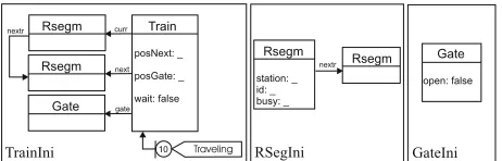
Figure 2. Initial Graphs Templates

(7)

Train wait: false

Traveling

Train wait: false

MayGo? t

R1-T

Train wait: false

Traveling

Train wait: true

R2-T

Wait

10

Train wait: b

Wait

Train wait: false

MayGo? t

R3-T

Train

posNext: n posGate: g next

Rsegm:N

Go

R4-T

n<>g

curr

Rsegm:C

Rsegm:X nextrs_xid

Rsegm:N curr

Rsegm:X

Rsegm:C

Train

posNext: x posGate: g

Traveling

10 next

Leaving

Train

posNext: n posGate: g wait: false Gate

Gate

Go

R5-T

n=g Rsegm:X nextrs_x id

Train

posNext: n posGate: g wait: true Gate

Gate

OpenGate Rsegm:Xnextrs

id

x

3 2

Open

Train

posNext: n posGate: g wait: true next

Rsegm:N

R6-T

curr

Rsegm:C

Rsegm:X

Rsegm:N curr

Rsegm:X

Rsegm:C

Train

posNext: x posGate: g wait: false

Traveling

10 next

Leaving OpenGate

nextrs id

x

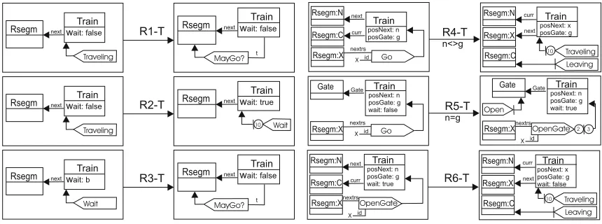
Figure 3. Train Rules

Gohave parameters. The initial graph templateTrainIni in Figure 2 describes that initially a train must be con-nected to two instances ofRSegm, one ofGate, and has a pendingTravelingmessage (this message will trigger the movements of the train). The attribute wait is ini-tialized tofalse. To create an object of this class, four arguments are need to instantiate this template: a natu-ral number (posGate), two railroad segments (currand next) and one gate (gate).

The behavior of the Train entity is modeled by the rules shown in Figure 3. RuleR1-Tdescribes that, when receiving a messageTraveling, a train tries to travel to the railroad segment pointed by itsnextattribute. This is modeled by the messageMayGo? at the right-hand side of the rule asking permission to enter this segment. Rule R2-Tchooses to wait at least 10 time units before trying to travel. Since both rules delete the same message, for each message, one will be non-deterministically chosen to be applied. RuleR3-Tmodels that, when receiving a Waitmessage, the train asks permission to enter the next railroad segment. RuleR4-Tdescribes the movement of a train: it updates its attributes, sends aTravelingmessage to itself to be received in (at least) 10 time units (simulat-ing the time needed to reach the end of this segment) and sends a message to the segment it was in to inform that this train is leaving. Note that this rule has a condition n<>g, expressing that this movement may only occur if there is no gategto enter the next positionn. If there is a gate, messageGowill be treated by ruleR5-T, that re-quires the gate to open immediately (theOpenmessage is scheduled to arrive exactly in the next time unit (with-out delay)). The application of ruleR5-Talso generates a messageOpenGate, that shall arrive between 2 and 3 time units (the time needed for the gate to open), and will trigger ruleR6-T, that will then move the train to the next position.

Railroad Segment Entity: this graph grammar is depicted in Figure 1 (type graph), Figure 2 (initial graph template RSegIni) and Figure 4 (Railroad Segment Rules). The type graph describes that each railroad seg-ment keeps the information about its identiﬁer (attribute id: Natural), its neighbour (the referencenextr), its state (busy:Boolean) and the knowledge whether it is a station or not (station:Boolean). The initial graph is given by two consecutiveRSegminstances. Instances ofRSegm can react to messagesMayGo?, telling a train that it can either move to it (ruleR2-R) or that it should wait at least 10 time units (ruleR1-R), and to messagesLeaving, up-dating itsbusyattribute (rule R3-R).

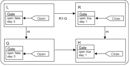
Gate Entity: the speciﬁcation of theGate Entityis shown in Figure 1 (type graph), Figure 2 (initial graph template GateIni) and Figure 4 (Gate Rules). The type graph indicates that gates have one attributeopenthat de-scribes whether the gate is opened or closed. By rule R1-G, if the gate is requested to open, its closure is scheduled to occur between 5 and 8 time units, i.e. all open requests cause a delay in closing the gate. By ruleR2-G, if the gate is opened and there is a close request, attributeopen is modiﬁed to false.

3. S

EMANTICS OF

T

IMED

O

BJECT

B

ASED

G

RAPH

G

RAMMARS

(8)

R1-R

Train

nextr

Rsegm

R2-R not(b) or s

R3-R Rsegm

busy:true station:false

Gate

open: false _Open R1-G

Train

MayGo? t

Rsegm

busy:true station:false

Train

Wait 10

Rsegm

busy:b id: x station:s

MayGo?

t _Train

nextr

Rsegm Rsegm

busy:not(b) id: x station:s

Go

nextrs id _x

Rsegm

busy:b

Leaving

Rsegm

busy:false

Gate

open: true 5 _Close

Gate

open: true _Close R2-G

Gate

open: false

Railroad Segment Rules Gate Rules

8

Figure 4. Railroad Segment Rules and Gate Rules

Rule Application, Computation. Given a rulerand a stateG, we say that this rule is applicable in this state if there is a matchm, that is, an occurrence of the left-hand side of the rule in the state. We denote suchrule applica-tionbyG(=r,m⇒)H.GraphsGandH are calledinputand

outputgraphs of this rule application. A rule application means that all items that are in the left-hand side of the rule and not in the right-hand side will be deleted from

G, and all items that are in the right-hand side ofr but not in its left-hand side will be included inG(formally, this effect can be described by a pushout in suitable cat-egories of graphs). In a graph, there may be various ver-tices/edges with the same types. This means that the same rule may be applicable to a graph using different matches. Acomputation of a graph grammaris a sequence of rule applications starting with the initial graph of the grammar, and in which the output graph of one rule application is the input graph of the next one. We say that a graph (or state) Gisreachableif there is a computation in which the output graph of the last rule application isG.

DEFINITION7 (RULE APPLICATION,COMPUTATION)

Let OBGG = (Spec, X, C, IG, N, n) be an object-based graph grammar,(r : L → R, Eq)be a rule, and G be a typed graph over C. A match for r in Gis a total morphism m : L → G in OBGraph(C). A rule

application G (=r,m⇒) H using rule rand match m is a pushout in the category OBGraph(C). The morphism r :G→His called derived rule.

L R

G H

r _/_/

_

m

r //

(P O)

A(ﬁnite) computationofOBGGfromIGtoH, de-noted byIG =∗⇒ H, is a sequence of rule applications Gi(r=i,m⇒i)Gi+1,i∈ {0, . . . , n},n∈N, whereG0=IG, Gn = H and ri ∈ Rules(C)for all i ∈ {0, . . . , n}.

Inﬁnite computations are deﬁned analogously, with i ∈

N. The class of all computations ofOBGG is denoted by CompOBGG. The class of all reachable graphs in

CompOBGG is deﬁned by StateOBGG = {G | G =

IG∨IG=∗⇒G∈CompOBGG}.

An example of a rule application is shown in Figure 5.

Gate

open: false

stay: 0 R1-G

Open Gateopen: true

stay: 1 Close

Gate

open: false stay: 0

Gate

open: true stay: 1

m m

L R

G H

Open Close

Figure 5. Example of a Rule Application

(9)

consideration any time restrictions. In order to deﬁne the transition system that gives semantics to a timed object-based graph grammar, we make an extension of the usual semantics, including clocks on states and allowing only rule applications that respect time restrictions.

Time is handled in the following way: a clock is assigned to each timed message, that is, to each message that is generated with some time constraint (minimum and/or maximum delivery time). This clock is initialized with zero, and, as time advances, the clock eventually reaches the minimum/maximum time. One requirement that is imposed on the semantic model is that all clocks advance simultaneously. This requirement implies that the relations among delivery times of messages in a state are preserved in the subsequent states, and this assures that the time constraints of the system are adequately modeled. Note that this does not impose a serious restriction in practice, since we are just assuming that clocks count the time in the same units and never stop until they are deallocated (in particular, this does not mean that we have a global notion of time).

Timed State. In the semantical model proposed here, states are described by tuples(G, ClocksG, mcG, valG), whereGis a timed object-based graph,ClocksGis a set of clock names, a functionmcGassociates a clock with each timed message ofG, and a functionvalGassociates a time (natural number) with each clock.

DEFINITION8 (TIMED STATE) Given a timed object

based graph grammarT OBGG= (Spec, X, C, IG, N, n) and a timed graph G over C. The tuple SG =

(G, ClocksG, mcG, valG) is called a timed state if (i)

ClocksG is a set of clock names; (ii) the partial

func-tionmcG :mEG → ClocksG, calledclock assignment function, is injective and total on timed messages of G; (iii) the total functionvalG : ClocksG →N, called in-terpretation or value function, assigns a time with each clock ofSG.

Timed Computations. A state change of a TOBGG can be obtained in two ways: by an application of a rule of a TOBGG or by elapse of time. In both cases, time restric-tions must be obeyed: in the case of rule applicarestric-tions, it must be assured that a message will be treated only within its delivery time (this is guaranteed by suitable deﬁnition of match for timed rules); in the case of time elapse, the maximum treatment time of all messages should not be violated (this is guaranteed by forbidding computations that would lead to inconsistent states, that is, states that do not satisfy the time restrictions). A timed computa-tion is deﬁned by a sequence of such state changes (cor-responding to rule application or time elapse). Therefore, by construction, a timed computation guarantees that time

restrictions will never be violated.

DEFINITION9 (TIMED RULE APPLICATION) Let

T OBGG = (Spec, X, C, IG, N, n)be a timed object-based graph grammar, (r : L → R, Eq) be a rule, and SG = (G, ClocksG, mcG, valG) be a timed

state. A match for r in SG is a total morphism

m:L →GinOBGraph(C)such that iftrigger(r)is a timed message then (i)valG(mcG(mE(trigger(r)))) ≥

tG_min(mE(trigger(r))); (ii)valG(mcG(mE(trigger(r))))

≤tGmax(mE(trigger(r))).

A timed rule application SG (=r,m⇒) SH using

rule r and match m generates a timed state SH =

(H, ClocksH, mcH, valH) obtained as follows: H

is the graph resulting from application of rule r at match m in graph G; ClocksH = ClocksG −

{mcG₍_m

E(trigger(r)))} ∪ {ci|iis a message created

inH}; for each timed messagemsgofmEH

mcH(msg) =

mcG(msg), ifmsgwas preserved byr cmsg , ifmsgwas created byr

and for each clock namec∈ClocksH corresponding to

a messagemsgofH

valH(c) =

valG(c) , ifmsgwas preserved byr

0 , ifmsgwas created byr

DEFINITION10 (TIMED COMPUTATION) A (ﬁnite)

timed computation of a timed object-based graph grammar T OBGG = (Spec, X, C, IG, N, n)between timed statesSIG andSH, denoted bySIG =∗⇒SH, is a

sequence of transitionsSGi

lab

=⇒ SGi+1,i ∈ {0, . . . , n},

n∈N, whereG₀=IG,SGn=SHandlabcan be:

(ri, mi) : in this case, Gi (r=i,m⇒i) Gi+1 must be a rule application of rulerat matchm;

δ: a non-negative value corresponding to the elapse of time from state SG_i to state SG_i₊₁. In this

case, SG_i₊₁ is obtained as follows: Gi+1 = Gi,

ClocksGi+1 = ClocksGi, mcGi+1 = mcGi, valGi+1(_c) =_valGi(_c) +_{δ, for all}_c∈_Clocks_G

i+1.

This transition may only occur in case the following restriction is satisﬁed: for all timed messagemsgof Giwith corresponding clockcmsg,

t≤tGi

max(msg), where

valGi₍_c

msg)< t≤valGi+1(cmsg).

Inﬁnite computations are deﬁned analogously, withi∈N. The class of all timed computations of T OBGG is de-noted byCompT OBGG. The class of all reachable graphs

inCompT OBGGis deﬁned byStateT OBGG={G|G=

(10)

Rsegm id: 4 busy: false station: false Rsegm id: 2 busy: false station: false Rsegm id: 3 busy: false station: true Rsegm id: 1 busy: false station: true nextr nextr nextr nextr Train posNext: 0 posGate: 4 wait: false curr next Gate open: false IG Traveling 10

mc : Traveling->clock1IG val :clock1->0IG

Rsegm id: 4 busy: false station: false Rsegm id: 2 busy: false station: false Rsegm id: 3 busy: false station: true Rsegm id: 1 busy: false station: true nextr nextr nextr nextr Train posNext: 0 posGate: 4 wait: false curr next Gate open: false G1 MayGo? Rsegm id: 4 busy: false station: false Rsegm id: 2 busy: false station: false Rsegm id: 3 busy: false station: true Rsegm id: 1 busy: false station: true nextr nextr nextr nextr Train posNext: 0 posGate: 4 wait: true curr next Gate open: false G2 Wait 10 R1-T R2-T Rsegm id: 4 busy: false station: false Rsegm id: 2 busy: false station: false Rsegm id: 3 busy: false station: true Rsegm id: 1 busy: false station: true nextr nextr nextr nextr Train posNext: 0 posGate: 4 wait: false curr next Gate open: false G0 Traveling 10 12

mc :Traveling->clock1G0 val :clock1->12G0

mc : Wait->clock2G2 val :clock2->0G2

Rsegm id: 4 busy: false station: false Rsegm id: 2 busy: true station: false Rsegm id: 3 busy: false station: true Rsegm id: 1 busy: false station: true nextr nextr nextr nextr Train posNext: 3 posGate: 4 wait: true curr next Gate open: false G6 Wait 10 Rsegm id: 4 busy: false station: false Rsegm id: 2 busy: true station: false Rsegm id: 3 busy: false station: true Rsegm id: 1 busy: false station: true nextr nextr nextr nextr Train posNext: 3 posGate: 4 wait: false curr next Gate open: false G7 MayGo? R3-T

...

mc : Wait->clock3G6 val :clock3->10G6

Figure 6. (Part of the) Transition System for the Railroad System

Semantics of TOBGG.

Now, the semantics of timed object-based graph grammars can be deﬁned: it is a transition system in which states are timed states and transitions correspond to rule applications that respect time restrictions (mini-mum/maximum delivery times of the message handled by the rule), or transitions that update clocks (all clocks si-multaneously). The latter should also respect message de-livery time restrictions: a clock can only be updated if the maximum time of the corresponding message is not vio-lated. By construction, this transition system corresponds to the class of all timed computations of a TOBGG.

DEFINITION11 (SEMANTICS OFTOBGG) Given a

timed object-based graph grammarT OBGG= (Spec, X, C, IG, N, n), its semantics is the transition system T S= (IS, States, Lab, T ran)deﬁned by:

Initial State: IS = (IG, ClocksIG, mcIG, valIG)

whereClocksIG = {cmsg|msgis a timed message

ofIG}; mcIG(msg) = cmsg, for all timed

mes-sages msg of IG; valIG(c) = 0, for all clocks c∈ClocksIG.

States: The set of states contains all states S that are reached by timed computations that is StatesT OBGG(see Def. 10).

Transitions: A transitionS1=lab⇒S2is inT ranif there exists a timed computationtcompofT OBGG start-ing atISthat contains this transition.

Lab : is the set of all labels of transitions inT ran.

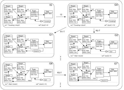
Figure 6 illustrates part of the transition system ob-tained for the Railroad System presented in Subsection 2.2. Rectangles represent states and arrows model tran-sitions (state changes). States are composed by a graph

(11)

R2-T. In the latter case,Travelingis the trigger message (it is consumed) and a timed messageWaitis created. The clock associated with this message,clock2, is initialized with zero.

To be able to perform automatic veriﬁcation of timed object-based graph grammars, we translate each TOBGG to an equivalent timed automaton, and use the existing tools to verify properties of timed automata to check the TOBGG. Since our semantic deﬁnition for TOBGG was highly inspired by timed automata, the comparison of the transition systems generated by TOBGG and timed au-tomata is straightforward.

4. T

IMED

A

UTOMATA

Timed Automata [1, 4] are used to specify and verify real-time systems. To express the behavior of a system with time restrictions, Timed Automata extend Nonde-terministic Automata with a ﬁnite set of clocks. In this model states and transitions are associated to clock con-straints. A clock constraint is a conjunction of atomic constraints, which compare clock variables with a con-stant value (a nonnegative rational value). Formally, letx

be a clock in a setClocksof clock variables andcbe a constant inQ, then the setφ(Clocks)ofclock constraints ϕis deﬁned by the grammar:

ϕ:=x≤c|c≤x|x < c|c < x|ϕ₁∧ϕ₂,

A clock constraint associated to a state (named in-variant) indicates how many time units the system may remain on a certain state. The constraint of a transition represents its activation conditions. Moreover, each tran-sition is associated to a set (possibly empty) of clocks that are reset with the occurrence of this transition.

DEFINITION12 (TIMEDAUTOMATON) A timed

au-tomatonT Ais a tuple(L, L0,Σ, Clocks, I, E), where: • Lis a set of states;

• L0⊆Lis a set of initial states; • Σis a set of labels;

• Clocksis a ﬁnite set of clocks;

• Iis a mapping that labels each statesinLwith some clock constraint inφ(Clocks);

• E ⊆ L×Σ×2Clocks×φ(Clocks)×L is a set of transitions. Each tuple(s, a, ϕ, λ, s)represents a transition from statesto a stateslabeled witha.ϕ is a clock constraint overClocksthat speciﬁes when the transition is enabled (it may be the empty con-straintε), and the setλ ⊆Clocksgives the clocks to be reset with this transition.

( a, ,{x} )e

( b,x>2,{ } )

s0 s1

_ x<4

Figure 7. Timed Automaton

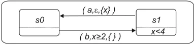
Figure 7 shows an example of a timed automaton wheres0 ands1represent the states of the system. The clock constraintx < 4in states1means that the system can remain in this state while the clock value xis less than four. The transitions are(s0, b, x ≥ 2,{ }, s1)and

(s1, a, ε,{x}, s0).

To each timed automatonT Awe can associate a cor-responding transition system [1]. The possible transitions are the ones speciﬁed in T A, and transitions that incre-ment the clocks (all clocks are increincre-mented simultane-ously). All transitions and reachable states must satisfy the time restrictions.

Formally, the semantics of a timed automatonAis de-ﬁned by associating a transition systemSAwith it. Each state ofSA is a pair(s, val), such thatsis a location of

Aandvalis a clock interpretation forClockssuch that

valsatisﬁes the invariantI(s). The set of all states ofA

is denoted byQA. A state(s, val)is an initial state ifsis an initial location ofAandval(x) = 0for all clocksx. There are two types of transitions inSA[1]:

Time elapse: for a state(s, val)and a real-valued time

δ≥0,(s, val)−→δ (s, val+δ)if for allδ≥δ ≥0,

val+δsatisﬁes the invariantI(s);

Automaton transition: for a state(s, val)and a transi-tion(s, a, φ, λ, s)such thatvsatisﬁesφ,(s, val)−→a

(s, val[λ:= 0]).

Thus,SAis a transition system with label-setΣ∪R.

5. T

RANSLATION OF

T

IMED

O

BJECT

B

ASED

G

RAPH

G

RAMMARS TO

T

IMED

A

U

-TOMATA

In this section we define formally how to obtain a timed-automaton that grasps this idea of behavior of timed OBGGs. If the initial state, the set of rules and the set of reachable states of a grammar are finite2_{, a finite}

timed automaton is generated. However, we can only deﬁne a timed automaton for grammars that reach states with a bounded number of messages (because the number of clocks in an automaton is ﬁxed). If we consider 2_{We assume that we have only one representative for each isomorphism}

(12)

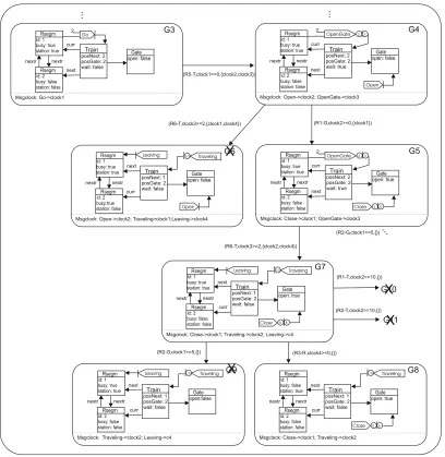
Rsegm id: 4 busy: false station: false Rsegm id: 2 busy: false station: false Rsegm id: 3 busy: false station: true Rsegm id: 1 busy: false station: true nextr nextr nextr nextr Train posNext: 0 posGate: 4 wait: false curr next Gate open: false IG Traveling Rsegm id: 4 busy: false station: false Rsegm id: 2 busy: true station: false Rsegm id: 3 busy: false station: true Rsegm id: 1 busy: false station: true nextr nextr nextr nextr Train posNext: 3 posGate: 4 wait: true curr next Gate open: false G6 Wait 10 Rsegm id: 4 busy: false station: false Rsegm id: 2 busy: true station: false Rsegm id: 3 busy: false station: true Rsegm id: 1 busy: false station: true nextr nextr nextr nextr Train posNext: 3 posGate: 4 wait: false curr next Gate open: false G7 MayGo? t Rsegm id: 4 busy: t station: false Rsegm id: 2 busy: false station: false Rsegm id: 3 busy:t rue station: true Rsegm id: 1 busy: false station: true nextr

nextr nextr nextr Train posNext: 4 posGate: 4 wait: false curr next Gate open: false G13 Go Rsegm id: 4 busy: t station: false Rsegm id: 2 busy: false station: false Rsegm id: 3 busy:t rue station: true Rsegm id: 1 busy: false station: true nextr

nextr nextr nextr Train posNext: 4 posGate: 4 wait: true curr next Gate open: false G14

OpenGate23 Open Rsegm id: 4 busy: t station: false Rsegm id: 2 busy: false station: false Rsegm id: 3 busy:t rue station: true Rsegm id: 1 busy: false station: true nextr

nextr nextr nextr Train posNext: 4 posGate: 4 wait: true curr next Gate open: true stay: 0 G15

OpenGate23 Close Rsegm id: 4 busy: t station: true Rsegm id: 2 busy: false station: false Rsegm id: 3 busy:t rue station: true Rsegm id: 1 busy: false station: true nextr nextr nextr nextr Train posNext: 2 posGate: 4 wait: false curr next Gate open: true stay: 0 G16 Traveling 10 Leaving TA

...

I(G14)clock2<=0 and clock3<=3 Msgclock: Go->clock1 I(G13)=clock1<=0 Msgclock:Open->clock2;OpenGate->clock3

Msgclock: Close->clock1;OpenGate->clock3 I(G15)clock3<=3 Msgclock: Close;->clock1;Traveling->clock2

(R5-T, clock1>=0; {clock2:=0,clock3:=0})

(R1-G, clock2>=0; {clock1:=0})

(R6-T, clock3>=2; {clock2:=0}) (R3-T, clock2>=10; {})

Msgclock: Wait->clock2

8 5

Close 58 10 Msgclock: Traveling->clock1

...

Rsegm id: 4 busy: false station: false Rsegm id: 2 busy: false station: false Rsegm id: 3 busy: false station: true Rsegm id: 1 busy: false station: true nextr nextr nextr nextr Train posNext: 0 posGate: 4 wait: false curr next Gate open: false G1 MayGo? Rsegm id: 4 busy: false station: false Rsegm id: 2 busy: false station: false Rsegm id: 3 busy: false station: true Rsegm id: 1 busy: false station: true nextr nextr nextr nextr Train posNext: 0 posGate: 4 wait: true curr next Gate open: false G2 Wait 10 Msgclock: Wait->clock2

(R1-T, clock1>=10; {})

(R2-T, clock1>=10; {clock2}) Rsegm id: 4 busy: false station: false Rsegm id: 2 busy: false station: false Rsegm id: 3 busy: false station: true Rsegm id: 1 busy: false station: true nextr nextr nextr nextr Train posNext: 0 posGate: 4 wait: false curr next Gate open: false G0 Traveling 10 Msgclock: Traveling->clock1 12

...

Figure 8. (Part of the) Timed Automaton for the Railroad System

ﬁnite-state systems (that are the ones that are possible to automatically verify), this imposes no restriction. To deﬁne this automaton, states are described by pairs

(G, msgclockG), whereGis a timed object-based graph andmsgclockGis deﬁned as follows:

Clock assignment function (msgclock): Given a graph

Gand a set of clocksClocks, the clock assignment functionmsgclockG : mEG →Clocksis a partial injective function that assigns a clock to each timed message of G(analogous to deﬁnition of function

mcin Def. 8);

x-tmessage bounded graph grammar: Grammar GG

isx-tmessage bounded, wherexis a natural number, if there is no reachable state ofGGin which there are more thanxtimed messages.

DEFINITION13 (TRANSLATION OFTOBGGTOTA)

Let T OBGG = (Spec, X, C, IG, N, n) be an

x-tmessage bounded timed object-based graph grammar. The translation of T OBGG to the timed automaton T A= (L, L0,, Clocks, I, E)is given by:

• L={(G, msgclockG)|Gis reachable inT OBGG andmsgclockGis a clock assignment function};

• L0= (IG, msgclockIG);

• =N×M or(timedOBGraph(C))3_;

• Clocks={clock₁, ..., clockx};

• I(G, msgclockG)is the conjunction of all formulas val(msgclockG(msg))≤tG_max(msg), withmsg∈ mEGandtGmax(msg)∈N;

• Eis the set of all transitions((G, msgclockG), a, ϕ, λ,(H, msgclockH))such that

3_Mor₍_timedOBGraph₍_C₎₎_{is the class of all morphisms in the}

(13)

Rsegm

id: 2 busy: false station: false

Rsegm

id: 1 busy: true station: true

nextr nextr

Train

posNext: 2 posGate: 2 wait: false curr

IG1

Rsegm

id: 2 busy: false station: false

Rsegm

id: 3 busy: false station: true

Rsegm

id: 1 busy: false station: true

nextr

Train2

posNext: 3 posGate: 1 wait: false

curr next

Gate

open: false IG2

Traveling 10

Msgclock: Traveling(Train1)->clock1;Traveling(Train2)->clock2 Msgclock: Traveling->clock1

Traveling 10

Train1

posNext: 2 posGate: 1 wait: false

curr

gate gate

Figure 9. Examples of Initial States

– ∃ a rule application G (=r,m⇒) H, let trigger(r) = msg and msgclockG(msg) = c;

– a= (r, m),

– ϕ=

⎧ ⎪ ⎪ ⎨ ⎪ ⎪ ⎩

(val(c)≥tG_min(msg)), iftL_min(msg) is deﬁned ε , iftL_min(msg)

is undeﬁned

– λis the set of clocks assigned to the timed mes-sages created by the rule application.

The clock constraint (invariant) (val(c) ≤ tmax(msg)) on states (I(s)) assures that the system may stay in statesat most until the clocks of all timed messages of s are less than their respective maximum time limits (because after this time, there will be at least one message in s that was not delivered in time). The clock constraint on transitionsϕassures that, if a message has a minimum time to be delivered (tL_min(msg)), it will not be processed before this time, if a message does not have such restriction, it may be processed at any time (the restrictions on maximum times for delivery are modeled by functionI, as described above). Moreover,λindicates which clocks shall be reset with the transitions, these are all the clocks used in the newly created timed messages in the target state of the transition.

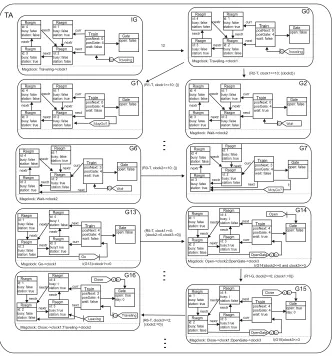
Now, this construction is illustrated by an example. Figure 8 shows a (partial) timed automaton (TA) that was obtained from translation of example in Subsection 2.2. The initial state ofTAis the stateIG.G1,G2,G6,G7, G13,G14,G15andG16are some states of the automa-tonTA(that are obtained with rules application fromIG). The time constraints were inserted following Deﬁnition 13. The complete timed automaton for this example has 36 states and 40 transitions. In the graph representations the matches are omitted.

Due to the construction of the timed automaton based on rule applications over reachable states of

T OBGG, this semantics is compatible with a tradi-tional semantics based on sequences of rule

applica-tions presented in Section 3: whenever there is a transi-tion((G, msgclockG),(r, m), ϕ, λ,(H, msgclockH))in the timed automaton, there is a corresponding transi-tion from graph G to graph H corresponding to ap-plying rule r using match m to graph G. The con-verse is also true because timed rule applications always respect the minimum/maximum delivery times of mes-sages, that is, a timed rule application SG (=r,m⇒) SH can always be translated to a corresponding transition

((G, msgclockG),(r, m), ϕ, λ,(H, msgclockH)), where the clock assignment functions are basically the same (up to renaming of the used clocks). Note that, in the TO-BGG transition system there is no limit in the number of created clocks, whereas in timed automaton there is a fixed set of clocks. Therefore, this full semantical com-patibility can be achieved only for grammars that do not generate an unbounded number of timed messages (since there is a clock for each timed message, such grammars would have to be translated to timed automata with infi-nite number of clocks, and this is not possible according do the definition of timed automata). The transitions that correspond to time elapse in both semantical models are defined basically in the same way: they must guarantee that maximum delivery times of messages will not be vi-olated. Thus, the resulting transition systems will have exactly the same time elapse transitions.

(14)

automa-Rsegm id: 2 busy: false station: false

Rsegm id: 1 busy: true station: true nextr nextr

Train

posNext: 2 posGate: 2 wait: false curr

G3

Msgclock: Go->clock1

Go

2

Rsegm id: 2 busy: false station: false

Train

posNext: 2 posGate: 2 wait: true curr

G4

Msgclock: Open->clock2; OpenGate->clock3

OpenGate

2

3 2

Open

(R5-T,clock1>=0,{clock2,clock3})

Train

posNext: 2 posGate: 2 wait: true curr

G5

Msgclock: Close->clock1; OpenGate->clock3

OpenGate

2

3 2

Close 5 8 Rsegm

id: 2 busy:true station: false

Train

posNext: 1 posGate: 2 wait: false next

curr

Gate open: false

G6

Msgclock: Open->clock2; Traveling>clock1;Leaving->clock4

Traveling

10

Open Leaving

(R1-G,clock2>=0,{clock1}) (R6-T,clock3>=2,{clock1,clock4})

X

Train

posNext: 1 posGate: 2 wait: false curr next

Gate open: true

G7

Msgclock: Close->clock1; Traveling->clock2; Leaving->c4

Close 58

Leaving 10 Traveling

Train

Gate open:false

G9

Msgclock: Traveling->clock2; Leaving->c4

Leaving 10 Traveling

X

Rsegm id: 1 busy: false station: true nextr nextr

Train

Gate open: true

G8

Msgclock: Close->clock1; Traveling->clock2

Close 58

Traveling

10 G10

X

G11

_X

(R3-R,clock4>=0,{}) (R2-G,clock1>=5,{})

(R1-T,clock2>=10,{})

(R2-T,clock2>=10,{})

...

(R6-T,clock3>=2,{clock2,clock4})

(R2-G,clock1>=5,{})

Figure 10. (Part of the) Timed Automaton for the Initial GraphIG1

ton has 123 states and 264 transitions. These numbers do not consider unreachable states and transitions.

6. V

ERIFICATION

For simulation and verification of properties of real-time systems we chose to use Uppaal (version 3.4.11) [3], a toolkit developed by Uppssala University and Aalborg University. Uppaal is a tool for validation (via graph-ical simulation) and verification (via automatic model-checking) that has timed automata as the input language and a subset of CTL as the specification language. The simulator can be used in three ways: the user can run the system manually and choose which transitions to

per-form, the random mode can be toggled to let the system run on its own, or the user can go through a trace (saved or imported from the veriﬁer) to see how certain states are reachable. The veriﬁer is designed to check a subset of CTL (Computation Tree Logic). The formulas to be checked must be in one of the following formats:

• A[]φ: for all paths,φalways hold;

• E <> φ: there exists a path where φ eventually holds;

• A <> φ: for all paths,φwill eventually hold;

(15)

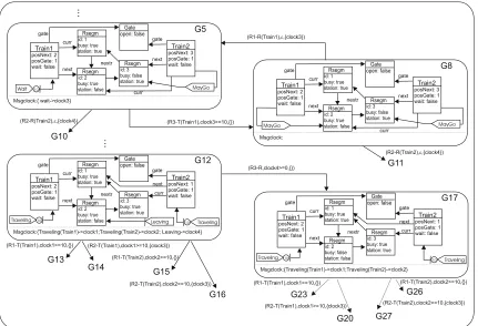
Rsegm id: 2 busy: true station: false Rsegm id: 3 busy: false station: true Rsegm id: 1 busy: true station: true nextr Train2 posNext: 3 posGate: 1 wait: false curr next Gate

open: false G5

MayGo Msgclock:{ wait->clock3} Train1 posNext: 2 posGate: 1 wait: false curr next Wait gate gate Rsegm id: 2 busy: true station: false Rsegm id: 3 busy: false station: true Rsegm id: 1 busy: true station: true nextr Train2 posNext: 3 posGate: 1 wait: false curr next Gate

open: false G8

MayGo Msgclock: Train1 posNext: 2 posGate: 1 wait: false curr next MayGo gate gate 10

(R1-R(Train1), ,{clock3})e

(R3-T(Train1),clock3>=10,{})

G10

(R2-R(Train2), ,{clock4})e

G11 Rsegm id: 2 busy: true station: false Rsegm id: 3 busy: true station: true Rsegm id: 1 busy: true station: true nextr Train2 posNext: 1 posGate: 1 wait: false curr next Gate

open: false G12

Leaving Msgclock:{Traveling(Train1)->clock1;Traveling(Train2)->clock2; Leaving->clock4} Train1 posNext: 2 posGate: 1 wait: false curr next Traveling gate gate 10 G13 (R1-T(Train1),clock1>=10,{}) Traveling 10 Rsegm id: 2 busy: false station: false Rsegm id: 3 busy: true station: true Rsegm id: 1 busy: true station: true nextr Train2 posNext: 1 posGate: 1 wait: false curr next Gate

open: false G17

Msgclock:{Traveling(Train1)->clock1;Traveling(Train2)->clock2} Train1 posNext: 2 posGate: 1 wait: false curr next Traveling gate gate

10 ₁₀ _Traveling

(R3-R,clock4>=0,{}) G14 (R2-T(Train1),clock1>=10,{clock3}) G15 (R1-T(Train2),clock2>=10,{}) G16 (R2-T(Train2),clock2>=10,{clock3}) ... ... (R1-T(Train1),clock1>=10,{}) (R2-T(Train1),clock1>=10,{clock3}) (R1-T(Train2),clock2>=10,{}) (R2-T(Train2),clock2>=10,{clock3}) G23 G20 G26 G27

Figure 11. (Part of the) Timed Automaton for the Initial GraphIG2

• φ− − > ψ: whenever φholds ψ will eventually hold.

where φe ψ are Boolean expressions that can refer to states, integer variables and clocks constraints. The word deadlockcan be used to verify deadlocks.

Safety properties mean that something bad will never happen. To check these properties in Uppaal, we use the formsA[]φorE[]φ. For example, the propertyA[] not deadlockwas checked for the railroad system of section 2.2 (with initial graph IG(Figure 8)) and was satisﬁed. This indicates the absence of deadlock for all paths of the system.

Reachability properties are the simplest forms of properties. They specify whether a given propertyφcan be satisﬁed in some reachable state. The formE <> φ

is used to check these properties. For example, we can check if there is one path in which stateG7of automaton TA in Figure 8 (that represents the situation when train asks permission to pass to the railroad segment identiﬁed with id 3) is reachable andclock2has a value less than 10 time units (E <> TA.G7 and clock2< 10). This property was checked and was not satisﬁed because when the system reaches stateG7, the value ofclock2must be already greater than 10 (this is the condition of the

transi-tion to reach this state).

Liveness properties are used to check if something good will eventually happen. These properties are ex-pressed by the forms A <> φ andφ− − > ψ. For example,TA.G13−−>TA.G16means that if stateG13 ofTAoccurs, thenG16will occur, too. This establishes that if the train can travel to a railroad segment that has a gate (situation represented by stateG13) the gate will eventually open and the train will travel to this segment (represented by stateG16). This property is satisﬁed by the example.

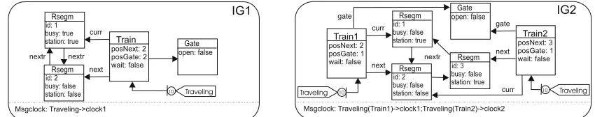
GraphIG1of Figure 9 illustrates a state with one train, two railroad segments and one gate. Considering this ini-tial state and the same rules for the behavior of trains, gate and railroad segments, we obtain a TOBGG whose corre-sponding timed automaton is partially depicted in Figure 10 . For this system, we veriﬁed the following properties:

• A[]not deadlock: the system never deadlocks, that is, in any reachable state, there is always a rule that can be applied.