© Swiss Journal of Economics and Statistics 2008, Vol. 144 (2) 117–151 Robert Aebia, Klaus Neusserb and Peter Steinerb,c
JEL-Classification: D31, C51
Keywords: income distribution, income dynamics, relative entropy
1. Introduction
Changes in the distribution of income in the US and elsewhere have kindled a lively debate on possible explanations. Special attention was given to the alleged decline of the middle income classes. Burkhauser, Cutts, Daly, and Jenkins (1999) addressed this issue by focusing on statistical inference and on measur-ing changes in the income distribution. They argue that sensible conclusions can only be drawn by comparing changes between years when the economy was in the same state with respect to the business cycle. Consequently, they compare the US income distributions at two peaks of the business cycle (i.e. in 1979 and 1989). Although they found significant increases in both tails of the distribution, the upper tail showed the largest gain by far. This picture is due to the fact that the authors looked at the problem from an absolute point of view in the sense that they did not control for economic growth.
The picture suggested by Burkhauser et al. (1999) remains incomplete, because their study does not shed any light on the underlying income process. An assessment of the increased inequality observed, however, must take into
* We thank Richard Burkhauser and Amy Cutts for providing us the data. We also want to thank the seminar and conference participants at the Institute for Advanced Studies in Vienna, Stanford University, ESEM 1999 and 2001, as well as Robert E. Leu and Edward Lazear for comments and suggestions.
a Institut de Recherche Mathématique Avancée, Université Louis Pasteur, 7 rue René Descar-tes, F-67084 Strasbourg Cedex, France.
b Department of Economics, University of Bern, Schanzeneckstrasse 1, Postfach 8573, CH-3001 Bern, Switzerland.
account the extent of mobility. Of course, this is easier said than done. The data attrition problem becomes severe because of the long time span between the two business cycle peaks. This makes it practically impossible to obtain a representative sample from a longitudinal database, like the Panel Study of Income Dynamics (PSID). In addition, income dynamics directly derived from panel data might be biased, because on average, individuals earn more when growing older.
To close this gap, we propose an alternative method that enables researchers to get estimates on the dynamics of income from cross-section information. To make our point clear, we will look at two closely related cases in the empirical section of this paper. First, we will adjust a theory based hypothesis of income dynamics in the light of cross-section information stated as income distributions observed at two points in time. We thus get estimates on the dynamics of income from cross-section information only. This proceeding enables researchers to shed light on the dynamics of income even in the absence of panel data information. Second, we draw the initial hypothesis on the dynamics of income from panel data. Here, our method is used to enhance the quality of regularly derived tran-sition matrices by incorporating information from cross-section databases, which usually cover a larger sample and therefore contain more information than panel data. In this case, our approach leads to a statistical test which can be used to draw inferences concerning the initial hypothesis. The test indicates whether the information inherent in the cross-section leads to statistically significant adjust-ments of the initial hypothesis. Because the adjustment is interpreted as a projec-tion, the adjusted dynamics, as seen from the initial hypothesis, is always “closer” to the true but unknown dynamics. We therefore always use the adjusted income dynamics to compute descriptive measures capturing important aspects of the evolution of the income distribution.
1 Aebi (1996, 1997) introduced the probabilistic approach into the mathematical literature. the advantage to avoid cumbersome optimization procedures, and automatically produces transition matrices.
Having presented our method in Section 2 of the paper, we apply our con-cepts to the same data as Burkhauser et al. (1999). Starting from three more or less plausible theory based hypotheses, we estimate transition matrices which map the 1979 into the 1989 income distribution. We also show how a transition matrix estimated from the PSID database must be adjusted in the light of the cross-section information contained in the very representative Burkhauser et al. (1999) sample. Finally, we discuss the properties of the adjusted transition matrices and their implications for the future development of the income distribution.
2. Methodological Foundations
2.1 A Probabilistic Model 1
Suppose we observe a large number of N distinguishable individuals, whose incomes develop independently, driven by the same unknown, discrete and time invariant Markov process. This means that the transition matrix P, representing the Markov process, doesn’t change over time. Starting with some initial income distribution at time 0 with density m0, the process is generating a time sequence of income-distributions represented by densities {mt}, t {1, 2, …}.
To simplify the presentation and in the face of empirical applications, these distributions are defined on a finite partition I {Ii}i 1, …, K of , making them discrete probability distributions mt. Thus, the income generating proc-ess conforms to a Markov chain with initial distribution m0. Consequently, {mt} {(mt,1, …, mt,K)'} is a sequence of (K v1)-vectors with properties:
mt,iu 0 i {1, …, K}, (1)
, 1
1, K
t i i
m
§
t {1, 2, …}.In the following, we assume that this sequence is observed at two points in time only, t and t1. Thus, incomes at the two points in time are distrib-uted according to the discrete probability distributions mt (mt,1, …, mt,K)' and
2 Even though this assumption seems to be unrealistic at first glance, it gets more plausible if we follow Champernowne (1953) and identify N as the number of incomes instead of individu-als. In Champernowne’s words, this means that “the incomes live on individually, although their recipients are transitory”. Alternatively, we could establish some “income class” 0. At t, class 0 consists of individuals that are present in t1 but not in period t (joining individu-als, “births”). At t1, only individuals that are present in period t but not in t1 belong to class 0 (leaving persons, “deaths”).
an individual income being in income class i in period t. In addition, it is sup-posed that no information concerning the true transition probabilities of the Markov process is available. We then ask the following questions: observing the cross-section distributions mt and mt1, what can be said about the individual dynamics (transition probabilities) and how should we modify any prior belief about individual dynamics?
If it were possible to observe the incomes of all individuals across time, it would be easy to count the number of individuals that are in income class i in period t and in income class j in period t1. Let’s denote these numbers by Jij and arrange them in a (K vK)-contingency table *:
, 1, ,
, 1
( ) with and [0, ]. K
ij i j K ij ij i j
N N
~
* J
§
J J (2)We will call this matrix income history matrix. * can be represented with the cor-responding 2-dimensional joint probability distribution (2-dimensional density matrix) D:
, 1, ,
(dij i j) K . N
*
D " (3)
Neither the true income history matrix *true nor the corresponding 2-dimensional density Dtrue are usually observable. It is solely known that they have to be com-patible with the observed true income distributions mt and mt1. In the following, we assume that nobody gets lost or is joining when passing from t to t1.2 Thus, each individual starting in some income class i must end up in some income class
j. Likewise, each individual ending up in some income class j must have started from some income class i. Thus, the income history matrix and the correspond-ing 2-dimensional density matrix have to meet the followcorrespond-ing restrictions:
, 1
{1, , }; K
ij t i j
N m i K
J ~
§
1,1
{1, , }; K
ij t j i
N m j K
J ~
, 1
{1, , }; K
ij t i j
d m ~i K
§
1,1
{1, , }. K
ij t j i
d m ~j K
§
In matrix notation and with the (Kv1)-vector L of elements 1, these restrictions simplify to:
1
1.
t t
t t
N m N m
m m
d
*L * L
d
L L
D D
(4)'
Because 6imt,i 1 and 6jmt1,j 1, the above conditions impose 2K 2 inde-pendent restrictions on * as well as on D, referred to as continuity restrictions or
initial and terminal conditions.
In general, these restrictions are fulfilled by an infinite number of income histories and corresponding 2-dimensional densities. All 2-dimensional density matrices compatible with the observed income distributions mt and mt1 con-stitute a convex subset D of the set of all 2-dimensional (KvK)-density matri-ces D (see Figure 1). Thus, the continuity restrictions can also be expressed in terms of set theory:
.
D D (4)''
The unknown true 2-dimensional density matrix, that is to be estimated, is an element of the set D. Because the true income generating process is unknown, a hypothesis or a model of this process is needed for periods t to t1. This hypothesis will be formulated in terms of a 2-dimensional density matrix
Dmod (dmod,ij )i,j 1, …, K. This model can be gained from empirical observations or theoretical reasoning and is generated either directly or even better, with a hypo-thetical transition matrix Pmod (pmod,ij)i,j 1, …, K. Because contrary to the 2-dimen-sional density, the transition matrix is time invariant by assumption, and because transition matrices are more common in economics, it seems convenient to gen-erate the hypothetical transition matrix Pmod in order to derive the density matrix
Dmod. Note that a given 2-dimensional density D unambiguously implies the cor-responding transition matrix P. Conversely, a given transition matrix P implies infinitely many corresponding 2-dimensional density matrices D. For each arbi-trarily chosen initial income distribution Pt (Pt,1, …, Pt,K)', Pt,ipmod, ij dmod, ij
3 Shortly, the solution is to take the observed true income distribution mt as initial distribution
of the hypothesis (see Section 2.2). Among other reasoning, this mixing of hypothesis and initial observation can be justified by the fact that the solution of the subsequent optimiza-tion problem has to comply with the continuity restricoptimiza-tions (4) anyway.
4 The field of application of the theory of large deviations is best outlined by means of a coin tossing thought experiment. Suppose a fair coin is going to be tossed N times. The probabil-ity of a rare event, e.g. more than 70% out of the N tosses yield head, decreases very fast when the number of tosses N is increased. The theory of large deviations is dealing with the speed at which the probability of such rare events tends to 0 when the number of observations (coin tossings N) is increased. In other words, this theory analyzes the behaviour in the tails of dis-tributions. The theory of large deviations could also be labelled as theory of rare events or is not distinct is identical with the indefiniteness of Pt, the initial distribution of the hypothetical dynamics of income. The solution to this problem of indefinite-ness is discussed in depth in Steiner (2004, pp. 33–36).3 With a chosen distri-bution Pt, the hypothetical 2-dimensional density matrix is given by
Dmod (dmod,ij )i,j 1, …, K (Pt,ipmod, ij)i,j 1, …, K diag(Pt)Pmod , (5)
where diag( Pt) is the diagonal matrix with the elements of Pt on the main diago-nal. Note that the hypothesis Dmod does not fulfill the continuity restrictions (4) in general. Dmod corresponds to the null hypothesis when it comes to statistical inference (see Section 2.3).
The continuity restrictions (4) are not sufficient to uniquely determine the income history * and the corresponding 2-dimensional density matrix, respec-tively. The problem to be solved could be described as follows:
Among all possibilities, we have to find the income history *opt or the corresponding 2-dimensional density matrix Dopt compatible with the continuity restrictions (4) on one hand and having maximal probability of being realized under the chosen hypothesis Dmod on the other.
This problem is going to be solved in two steps. First, we compute the probabil-ity for some distinct income history * to be realized under the chosen hypothesis
theory of analyzing the tail-distributions. The probability of realization of such rare events tends to 0 at an exponential rate. This exponential rate of convergence is of eminent interest in the theory of large deviations.
2.1.1 Probabilities of Income History Matrices
Assume that individual incomes evolve independently from each others. We will now compute the probability that a given income history *, compatible with restrictions (4), is going to be realized by N individuals from the viewpoint of the hypothesis Dmod. This given income history * can be realized in different ways by N individuals. At first, we will compute the number n(*) of distinct possibilities to realize *. This number corresponds to the number of possibilities to arrange N distinct individuals in subgroups of Jij persons. Elementary com-binatorics yields:
11 12
11
13
11 12
1 1 1
1
1 1 1 1
21
, 1
( )
! . !
K K K K
j ij Kj
K
j i j j
KK ij
i j N
N N
n
N N N
¨ ¸
¨ ¸¨ J ¸ J J
* © ¹©ª ºªJ J ¹©ºª J ¹º
¨ ¸ ¨ ¸
© J ¹ © J J ¹
© ¹ © ¹
© J ¹ © J ¹ J
ª º ª º
§
§§
§
"
" (6)
Because individuals are distinguishable, the history * could be realized by N
individuals in n(*) ways. From the viewpoint of hypothesis Dmod, we will now compute the probability Pr(*) of realization of one specific member out of these
n(*) possibilities. As usual with multinomial distributions, this probability is given by:
, mod, ij mod,
, 1 , 1
Pr( ) ( p )ij ( ) .ij
K K
t i ij
i j i j
d
J J
*
P
(7)Thus, each of the n(*) specific possibilities of realizing income history * has probability Pr(*) of being realized under hypothesis Dmod. From a macroeco-nomic point of view, we are not interested in any specific realization of history
5 See Schrödinger 1931 and Lanford 1973.
6 Chapter I in Ellis (1985) provides an insightful introduction to the concepts we will use subsequently.
mod mod,
, 1
, 1
mod,
, 1
!
Pr ( | ) Pr( ) ( ) ( ) !
( )
! .
!
ij
ij
K
N K ij
i j ij i j
K ij
ij i j N
n d
d N
J
J
* * *
J
J
D
(8)
2.1.2 Minimization and Optimally Adjusted Dynamics
Infinitely many income history matrices * or 2-dimensional densities D are com-patible with the continuity restrictions (4). Out of this set and from the view-point of the hypothesis, we have to unambiguously identify the most probable income history or 2-dimensional density respectively. To do this, we deploy the
fundamental hypothesis of statistical mechanics to the evolution of incomes. This general principle from particle physics means:
An observation on a macroscopic level (e.g. marginal distributions) is realized in the limit of infinitely many particles (e.g. individuals) by that microscopic ensemble (e.g. N-samples with N pf), which has maximal probability given the observation.5
Thus, we seek the income history which satisfies the continuity restrictions and which has, from the viewpoint of our hypothesis, the highest possibility of being realized.6
As already mentioned, the law of large numbers implies that every income history matrix that is compatible with the continuity restrictions has, from the perspective of our hypothesis, probability zero of being realized as N tends to infinity:
PrN(*|Dmod) p 0 , for Npf . (9)
7 We denote the natural logarithm throughout this paper with log. 8 Stirling’s formula is: ! ( )n 2 (1 ) with 0 for .
n n
n n e S Hn e p npg
9 The formula suggests generating hypothetical 2-dimensional densities Dmod without any zero
elements because computing the relative entropy of some arbitrary matrices with respect to such a hypothesis always yields non-infinite results. If the hypothesis contains 0’s, the opti-mally adjusted matrix has to inevitably exhibit 0’s at the same matrix-positions. Otherwise, the relative entropy that should be minimized by the method is going to be infinite. To exclude zero elements in hypotheses generated from real data, the technique to be used in these cases is 2-dimensional kernel estimation.
(1/N)log[PrN(*|Dmod)].7 Using Stirling’s formula for large factorials,8 this limit is given by:
mod mod
1
lim log Pr ( |N ) ( | ) with .
NpgN H N
* « »
* D ½ D D D (10)
The function H(D|Dmod) is known as relative entropy or Kullback-Leibler diver-gence of the 2-dimensional density D with respect to the hypothesis Dmod. It is defined as follows:
mod
mod,
, 1
0 ( | ) log with 0 log 0
0
and log . 0
K
ij ij
ij i j
ij ij
d
H d
d
d d
¨ ¸ ¨ ¸
© ¹
© ¹ © ¹ª º
ª º
¨ ¸
© ¹ g
ª º
§
D D
9 (11)
Because PrN(*|Dmod) converges exponentially fast to zero at rate (11) for large N, the function H(D|Dmod) is also called rate function.
mod
( )
mod
Pr ( | ) N N H .
N e
pg
* D|D
D (12)
The relative entropy has the following properties:
– H(D|Dmod) u0; nonnegative function of D.
– H(D|Dmod) 0 if and only if D Dmod.
10 Further properties of the relative entropy and a deeper discussion of its interpretation can be found among others in Kullback (1959) and Ellis (1985). By definition, a metric or distance function M(,) is nonnegative, symmetric in its arguments, fulfills the triangular inequality and has the property, that M(x,y) 0 if and only if x y.
– H(D|Dmod) has a global minimum in D.
– H(D|Dmod) { H(Dmod|D) ; no symmetry in its arguments.
The relative entropy does not define a metric in the space of probability distri-butions because it is not symmetric in its arguments and because it violates the triangular inequality.10 However, it is possible to give the relative entropy a geo-metric interpretation analogous to the common Euclidean distance. In particular and most relevant for this paper, the minimization of the relative entropy with respect to a given probability distribution Dmod over a convex subset D of prob-ability distributions can be viewed as a projection with properties similar to the projection in Euclidean or Hilbert spaces (Csiszár 1975). The relative entropy is some kind of “directed measure of distance” between two densities. This rela-tion is shown in Figure 1.
Figure 1: Geometry of the Csiszár Projection
. hypothesis
Dmod
H(Dtrue|Dmod)
H(Dtrue|Dopt) D
true
unknown “truth” Dopt
projection
H(Dopt|Dmod)
D–
D– = convex set of all twodimensional (KvK)-density matrices D with marginal densities mt and mt1
The analogy of the relative entropy and the Euclidian geometry becomes obvi-ous if we look at Figure 1 and note that the relative entropy fulfills the following analogon to the theorem of Pythagoras,
11 See Csiszár (1975) for a more detailed discussion.
where Dtrue is the true but unknown income dynamics in the form of a 2-dimen-sional density matrix. Dtrue could be replaced by any element of D, equation (13) is going to hold.11 In addition, Figure 1 shows that in terms of relative entropy, the optimally adjusted dynamics Dopt is at least as close to the true but unknown density Dtrue as the hypothetical dynamics Dmod.
From the viewpoint of our hypothesis, the relative entropy can be interpreted as a measure of probability of observing a certain income history matrix compat-ible with the given marginal distributions. The principle of statistical mechanics then advises us to take the “most probable” income history matrix subject to the continuity restrictions. We are thus led to consider the following “ill posed pure inverse problem” (Golan, Judge and Miller 1996):
Minimize H(D|Dmod ) over all 2-dimensional densities D subject to the continuity restrictions (4).
Of course, the set D of all 2-dimensional densities D compatible with restriction (4) contains infinitely many elements. If the convexity of the set D is taken in account, the 2-dimensional density Dopt (Dopt, ij)i,j 1, …, K, that is the most prob-able realization fulfilling restriction (4), can be determined as the Csiszár projec-tion of the hypothesis Dmod on D (Csiszár 1975). This projection is computed by minimizing the relative entropy over all elements of D with respect to Dmod:
mod
mod,
, 1
arg min ( | ) arg min log . K
ij
opt ij
ij i j
d
H d
d
¨ ¸
© ¹
©ª ¹º
§
D D
D D D
D D
(14)
If the minimizing problem (14) is solvable, the solution is going to be unique because the relative entropy H(|Dmod) is a nonnegative and strictly convex function.
In the words of the statistics literature, we have to find the minimum discrim-ination information under the hypothesis Dmod (Kullback 1959, p. 37). The solution is called the “minimum discriminant information adjustment” of Dmod
12 I.e. Dmod,ij 0 implies Dopt,ij 0. From (11) follows that the relative entropy of all matrices
D, not absolute continuous with respect to the hypothesis, is going to be infinite. To avoid this, Dopt must have zeros at the same positions as the hypothesis Dmod. Hence, it is
advan-tageous to generate the hypothesis without zero-elements to get the most realistic solution when adjusting the hypothesis to the observed marginal densities. This also proves beneficial in view of the iterative proportional fitting procedure (IPFP, see Section 2.1.3 and Deming and Stephan (1940)), which is going to be used as the solving algorithm. This algorithm is easier implemented and always yields a unique solution when using strictly positive hypoth-eses (Sinkhorn, 1967).
, ,
mod,
, 1 1 1
1, 1,
1 1
L log
,
K K K
ij
ij t i ij t i ij
i j i j
K K
t j ij t j
j i
d
d d m
d
d m
¨ ¸
¨ ¸
© ¹
© ¹
© ¹ O © ¹
ª º ª º
¨ ¸
© ¹
O
ª º
§
§
§
§
§
(15)where Ot,i and Ot1,j are the 2K Lagrangian multipliers associated with the con-straints (4). A solution to this optimization problem exists if and only if there is at least one income history matrix that satisfies the continuity restrictions (4). In addition, this matrix has at least the same zero entries as the hypothesis
Dmod (Csiszár 1975, corollary 3.3), i.e. the solution has to be absolute continu-ous with respect to the hypothesis.12 To solve the optimization problem, the set
D has to contain at least one element that is absolute continuous with respect to the hypothesis. The strict convexity of the relative entropy then implies the uniqueness of this solution. This solution Dopt is found by differentiating (15) with respect to dij and by setting the resulting derivatives equal to zero (first order conditions):
,
1 1,
opt, , mod, 1, ,
1,
, {1, , }, with
and .
t i
t i
ij t i ij t j t i
t j
d d i j K e
e
O
O
I I ~ I
I (16)
With It (It,1, …, It,K)' and It1 (It1,1, …, It1,K)', equation (16) can be writ-ten more compactly in matrix notation:
Dopt diag(It)Dmoddiag(It1). (16)'
From the viewpoint of the hypothesis, Dopt characterizes the most probable esti-mation of the true but unknown dynamics of income generation.
In the theory of quantum mechanics, the I’s are known as Schrödinger multipli-ers (Aebi and Nagasawa 1992). They indicate how to adjust “in the most probable way” the 2-dimensional density Dmod, representing our hypothesis about income dynamics, to satisfy the continuity restrictions (4). The Schrödinger multipliers adjust the probabilities Dmod, ij of our hypothesis downward, if It,iIt1,j 1, and upward, if It,iIt1,j! 1. The matrix ItIt1' may therefore reveal patterns of adjustment and indicates the entries, where our hypothesis is misspecified. In addition, the Schrödinger multipliers contain some kind of “time separability property” because the It,i depend only on the initial distribution mt, whereas the
It1,j depend only on the final distribution mt1 (see equations (15) and (16)). The relative size of It and It1 thus indicates whether the misspecification is primarily due to the initial or to the terminal restriction.
The Schrödinger multipliers are found after differentiating L (equation (15)) with respect to the Lagrangian multipliers (Ot,i and Ot1,j respectively) and set-ting the derivatives equal to zero. The resulset-ting equation system is the so-called
Schrödinger system:
, , mod, 1,
1
, , mod, ij 1,
1
1, , mod, 1,
1
, , mod, ij 1,
1
p 1, ,
p 1, , .
K
t i t i ij t j j
K
t i t i t j j
K
t j t i ij t j i
K
t i t i t j i
m d
i K
m d
j K
I I
I P I ~
¨ ¸
© I ¹I
ª º
¨ ¸
© I P ¹I ~
ª º
§
§
§
§
(17)This equation system shows that the Schrödinger multipliers are unique only up to a multiplicative constant. In the following we normalize the I’s such that
It,1 It1,1.
the 2-dimensional density and the corresponding transition matrix are related by Dopt,ij mt,ipopt,ij. The elements of Popt are therefore derived from the hypo-thesis Pmod as follows:
opt, , mod, 1,
opt, ,
, mod, 1,
1
, , mod, 1, mod, 1,
, , mod, 1, mod, 1,
1 1
. ij t i ij t j
K ij
t i
t i ij t j j
t i t i ij t j ij t j
K K
t i t i ij t j ij t j
j j d d p m d p p p p
I I
I I
I P I I
I P I I
§
§
§
(18)In matrix notation, equation (18) summarizes to:
i
i
1
opt 1 mod 1
mod,1 1, mod, 1,
1
1 1
( ) ( )
with , , .
t t
K K
j t j Kj t j t j j diag diag p p
I I
d
¨ ¸
© ¹
I © I I ¹
ª
§
§
ºP P
" (18)'
Note that Popt satisfies the definition of a transition matrix, i.e.
popt,iju 0 and K 1 opt, 1 ij j p
§ for all i.
Moreover, Popt is obtained from Pmod only through the Schrödinger multipliers It1,j related to the terminal restrictions. The adjustment factors are now given by
i 1
1, ,
1,
( t i t j i j) .
I I As with the 2-dimensional density, the optimally adjusted tran-sition matrix Popt results from multiplying each pmod,ij with its corresponding adjustment factor.
2.1.3 Iterative Proportional Fitting Procedure (IPFP)
13 Compared with Sinkhorn (1967, 1964), the analogies '1 diag(It) and '2 diag(It1)
hold.
14 A zero element in Pt produces a row of zeros in the hypothesis Dmod, which stops the IPFP
method in step 1.
of a (KvK)-contingency table with known and given marginal distributions
mtand mt1. This problem was first treated by Deming and Stephan (1940). They suggested the IPFP method to solve this optimization problem. The pro-ceeding is an iterative one:
1. By element-wise division of the observed initial distribution mt with Pt, the vector of row-sums of Dmod, we compute the vector Tt.
2. The first estimation of Dopt is computed according to D1 diag(Tt)Dmod. The row-sums of the resulting density D1 are identical with mt.
3. Element-wise division of the observed final distribution mt1 with Pt1, the vector of column-sums of D1, generates the vector Tt1.
4. The second estimation of Dopt is computed according to D2 D1diag(Tt1). The column-sums of D2 match mt1.
5. Like in step 1, Pt and Tt are computed where Pt is now the vector of row sums of D2 instead of Dmod. Concretely, steps 1 to 4 are repeated with the 2-dimen-sional density of the respective prior step until this process converges.
Sinkhorn (1967, 1964) proved that this process of alternated adjustments of the row- and column-sums of a positive matrix X to prescribed row- and column-totals respectively, always converges towards a positive matrix X '1X'2, where '1 and '2 are diagonal matrices. In addition, he proved that this conver-gence is unique and that both diagonal matrices are unique up to a multiplica-tive constant.
In our terminology, this means that applying the IPFP method to Dmod leads to convergence against the matrix diag(It)Dmoddiag(It1), that is, according to (16)', identical with Dopt, the sought-after solution of the optimization prob-lem (14).13 Thus, the IPFP method always converges for positive 2-dimensional densities Dmod. According to Dmod diag(Pt)Pmod, this implies that both, the hypothetical transition matrix Pmod as well as the chosen initial distribution Pt have to be positive to guarantee the convergence of the IPFP method, where
Pt!! 0 is essential for convergence.
14 The positiveness of the hypothetical
tran-sition matrix Pmod is not essential, but as we have seen earlier, there are reasons why positive hypotheses are advantageous.
likelihood estimates and that these estimates minimize the relative entropy (11) (Smith 1947; Ireland and Kullback 1968).
2.2 Choosing Best Possible Hypothetical Density Matrices
In the following, it is assumed that the hypothetical Markov chain is set by choos-ing the correspondchoos-ing transition matrix Pmod. As mentioned in Section 2.1, there exists an infinite number of 2-dimensional density matrices that are compatible with the given transition matrix Pmod and thus could be used as a starting point to determine optimally adjusted densities Dopt and corresponding transition matri-ces Popt respectively. All these hypothetical density matrices compatible with the chosen transition matrix Pmod constitute a convex set labeled Dmod(Pmod) :
mod( mod) { mod mod diag( )P mod and P!!0}.
D P D D P (19)
When it comes to pinpoint the hypothetical density Dmod, a problem of indeter-minacy arises. At this point, there are two questions of interest:
– Given the hypothetical transition matrix Pmod, how is the choice of the arbi-trary initial distribution Pt and thus the hypothetical 2-dimensional density
Dmod affecting the resulting adjusted dynamics Dopt ?
– Is it generally possible to solve this indeterminacy problem in a satisfactory way and if yes, how do we have to proceed?
Steiner (2004, pp. 33–36) proved that the optimally adjusted dynamics Dopt
and Popt, respectively, are not affected by the choice of the initial distribution
Pt!! 0. Given the hypothetical transition matrix Pmod, every Pt!! 0 and thus every corresponding hypothetical density Dmod yield the same optimally adjusted dynamics. In addition, he showed that of all members of the set Dmod(Pmod), the
hypothesis generated from the observed initial distribution mt lies, in terms of relative entropy, closest to the set D of all 2-dimensional densities D com-patible with restriction (4) and thus closest to the true but unknown dynam-ics Dtrue. Because it is the only hypothesis that lies this close to D, it is spe-cially labeled mod diag m( t) mod
D P to distinguish it from the other possible hypotheses.
Hence, Steiner suggests to determine the hypothetical dynamics in a two step procedure:
a priori. If no income panel is at hand, there is always the possibility to gener-ate the hypothetical transition matrix from theoretical reasoning. Besides the fact that theory based hypotheses are always open to criticism, they have the advantage to be at hand in any situation.
2. Pre-multiplication of the hypothetical transition matrix with the diagonal matrix generated from the observed initial distribution according to Dmod
diag(mt) Pmod.
2.3 Statistical Inference
From a statistical point of view, we do not only want to know how to best adjust our hypothesis to given data, but also whether these adjustments are significant in a statistical sense. Ireland and Kullback (1968) show how to test the statis-tical significance of these necessary adjustments of the hypothesis to the observed marginal distributions. If the hypothesis Dmod is generated directly from a sample of n individuals, the statistics
2
opt mod 2 2
2 n H(D |D ) ~F K (20)
is asymptotically F2-distributed with 2K2 degrees of freedom. According to Ireland and Kullback, the number of degrees of freedom is given as the difference in the numbers of degrees of freedom of the unrestricted model Dmod (K21) and the restricted model 2
((K 1) (2 K 2)).
D D Thus, the number of
degrees of freedom is equivalent to the number of restrictions in (4).
If the hypothetical transition matrix Pmod is generated from a sample of n indi-viduals and the hypothetical 2-dimensional density, incorporating the observed true initial distribution, is built according to mod diag m( t) mod,
D P the test statistics
2
opt mod 1
2 n H( | ) ~ K
D D F (21)
is asymptotically F2-distributed with just K 1 degrees of freedom. Again, the number of degrees of freedom is calculated from the difference of the respective numbers in the unrestricted and the restricted models. The number of degrees of freedom of the unrestricted model Dmod is (K21)(K1) K2K. The respective number of the restricted model DD is (K21)(2K2)
K22K1. Hence, we obtain the resulting K1 degrees of freedom in test statistics (21).
of the test statistic indicates that significant adjustments to the initial hypoth-esis are necessary. Because the adjusted matrix is always closer to the unknown true dynamics than the hypothesized one, we always use the adjusted transition matrix for the evaluation of income dynamics (e.g. mobility indices, projections in the future, etc.).
Of course, the literature proposes several alternative methods to extract infor-mation on transition probabilities from cross-section observations (for exam-ple Adelman, Morley, Schenzler, and Warning 1994; Golan, Judge, and Miller 1996; Kalbfleisch and Lawless 1984; Lee, Judge, and Zellner 1970). Our approach, however, has several important advantages over these alter-natives. First, because we observe the distribution only at two points in time, there are more unknown elements in the transition matrix P (respectively in the density D) than observations in the restrictions. We are thus facing an ill-posed inverse problem which precludes the application of least-squares estimation. In this situation the maximum entropy principle arises as a natural criterion (Golan, Judge, and Miller 1996). Second, our approach together with the IPFP guaran-tees that the resulting adjusted matrices Dopt and Popt are 2-dimensional densities and transition matrices respectively. Thus we can avoid cumbersome constrained minimization problems. Third, although our approach requires the specification of a hypothesized density Dmod, this is not restrictive because setting all elements of Dmod equal to 1/K 2 results in a non-informative prior. Finally, the minimization by the iterative proportional fitting procedure is robust and easy to implement.
3. Empirical Results
We are now in a position to apply the method described in the previous sec-tion to real data. In order to gain informasec-tion on the unobserved process of income dynamics from cross-section data, our approach needs the following two ingredients:
Income distributions observed at two points in time. These distributions are labeled m1979 and m1989 respectively. They are extracted from the Current Popu-lation Survey (CPS).
An initial hypothesis of the process of income dynamics. This hypothesis is stated in the form of a transition matrix Pmod or equivalently, by incorporating the information inherent in the initial distribution m1979, as a 2-dimensional density matrix Dmod.
adjusted 2-dimensional density Dopt. The adjusted transition matrix is then used to gain information on the process of income dynamics such as mobility meas-ures, projections into the future and measures of inequality.
For our empirical investigation we used the same data as Burkhauser et al. (1999). These data come from the Current Population Survey (CPS) and are based on pre-tax post-transfer household incomes measured in 1989 US dollars. In contrast to Burkhauser et al., we controlled for overall economic growth by adjusting the 1979 data with the mean of the 1989 data. The household income is converted to individual income using an equivalence scale with 0.5 elasticity (square-root scale). In all our calculations we also take into account the weight associated with each sample observation. For the sake of exposition, we have re-estimated the densities of the income distributions in 1979 and 1989 using the adaptive kernel density estimator described in Silverman (1986) and adopted by Burkhauser et al. (1999). The estimates are plotted in Figure 2. They clearly document the relatively large decline of the middle to upper middle income classes with a corresponding increase of the highest and lowest income classes.
Figure 2: Income Distribution in the US (Mean Adjusted), Individual Equivalent Pre-Tax Post-Transfer Household Income
0 10 000 20 000 30 000 40 000 50 000 60 000 70 000 3.5
3.0
2.5
2.0
1.5
1.0
0.5
0 ×105
As our approach is based on a finite state space, we partitioned the real line into K
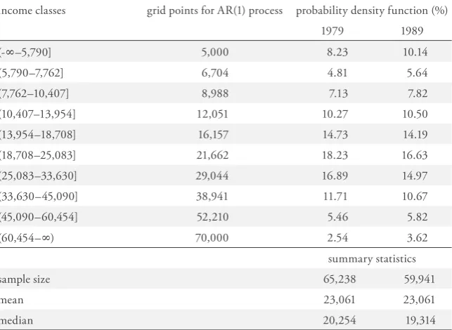
intervals. We have chosen K arbitrarily equal to 10 presuming that this is enough to capture the main characteristics of the income process. Furthermore we have fixed the boundaries of the intervals in such a way that they are of equal length on a logarithmic scale, except the first and the tenth interval, of course. The resulting partition is documented in Table 1 which also shows how the incomes are distributed into the income classes in the years 1979 and 1989.
Table 1: Income Classes and Corresponding Probability Density Functions
income classes grid points for AR(1) process probability density function (%)
1979 1989
(-g–5,790] 5,000 8.23 10.14
(5,790–7,762] 6,704 4.81 5.64
(7,762–10,407] 8,988 7.13 7.82
(10,407–13,954] 12,051 10.27 10.50
(13,954–18,708] 16,157 14.73 14.19
(18,708–25,083] 21,662 18.23 16.63
(25,083–33,630] 29,044 16.89 14.97
(33,630–45,090] 38,941 11.71 10.67
(45,090–60,454] 52,210 5.46 5.82
(60,454–g) 70,000 2.54 3.62
summary statistics
sample size 65,238 59,941
mean 23,061 23,061
median 20,254 19,314
15 Prais’ mobility index is defined as (Ktr(P)) (K1) (Prais 1955).
The critical issue is to specify a reasonable hypothesis Dmod. In order to encom-pass alternative views on the dynamics of the income process, we have investi-gated three “theory” and one empirically based specifications Pmod. We chose the observed initial distribution m1979 to transform the hypothetical transition matri-ces Pmod into the corresponding hypothetical 2-dimensional densities Dmod. Thus we are left with the specification of the hypothetical transition matrices Pmod.
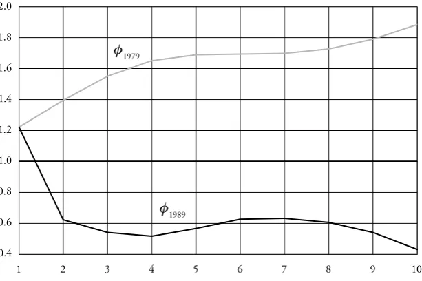
Each specification is presented in a separate table together with the corre-sponding adjusted transition matrix Popt. Each table is linked to a Figure where the associated Schrödinger multipliers I1979 and I1989 are plotted. Although the Schrödinger multipliers corresponding to the initial conditions are not necessary for the calculations of the adjusted transition matrices, they are nevertheless plot-ted to give a more complete picture and because we always have to compute them in an intermediate step of the iterative proportional fitting procedure (IPFP).
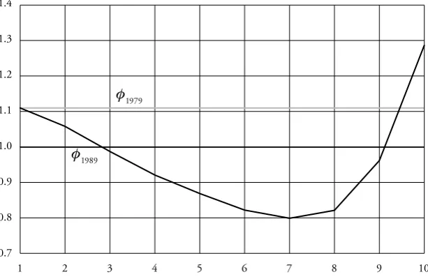
The first specification starts from a transition matrix P with maximum mobil-ity. These are transition matrices where the probability of attaining a certain income class is independent from the initial income class (Prais 1955). These transition matrices thus have equal rows so that their Prais’ mobility index equals 1.15 It can be shown that our entropy approach adjusts any transition matrix with maximum mobility in such a way that it becomes equal to a matrix with rows equal to Dmod. Moreover, using the normalization It,1 It1,1 and taking P equal to mt, the Schrödinger multipliers related to the initial restric-tion are constant and equal to
,1 1,1 ,1.
t mt mt
I
The Schrödinger multipliers related to the terminal restrictions then become
1, ,1 1,1 ( 1, , ).
t j mt mt mt j mt j
I
16 Of course, there are infinitely many 3-band transition matrices preserving a given density. Our construction follows the recommendation of Boyarsky and Góra (1997, 258). to be reduced whereas the probabilities of moving into the highest and lowest income classes have to be increased.
Figure 3: Schrödinger Multipliers for the Maximal Mobility Hypothesis
1 2 3 4 5 6 7 8 9 10
I1989
1.4
1.3
1.2
1.1
1.0
0.9
0.8
0.7
I1979
The second “theory” based hypothesis represents a more interesting specification. Suppose that individuals cannot move more than one class up or down from one year to the next. This implies that the one period hypothetical transition matrix is a 3-band matrix denoted by P3band. Suppose further that the observed distribution in 1979, m1979, is invariant to P3band.16 Taking P m1979 as before, the joint prob-ability density function D3band over the decade 1979 to 1989 is then given by
10
3band diag(m1979) 3band
D P (22)
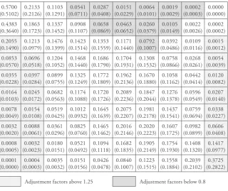
several interesting features. First the probability of staying in the lowest income class is with 0.51 relatively high. Even for the next two income classes, there is a substantial probability of falling back into the lowest class. From class three to five, the probability of moving up clearly outweighs the probability of falling down. This changes from class seven on where the chances of falling down are now higher than the chances of moving up further.
Table 2: Hypothesized and Adjusted Transition Matrix for the 3-band Hypothesis
0.5700 (0.5102) 0.2133 (0.2126) 0.1103 (0.1291) 0.0541 (0.0711) 0.0287 (0.0408) 0.0151 (0.0229) 0.0064 (0.0101) 0.0019 (0.0029) 0.0002 (0.0003) 0.0000 (0.0000) 0.4383 (0.3640) 0.1863 (0.1723) 0.1337 (0.1452) 0.0908 (0.1107) 0.0658 (0.0869) 0.0463 (0.0652) 0.0260 (0.0379) 0.0105 (0.0149) 0.0022 (0.0026) 0.0002 (0.0002) 0.2055 (0.1490) 0.1213 (0.0979) 0.1476 (0.1399) 0.1423 (0.1514) 0.1353 (0.1559) 0.1171 (0.1440) 0.0792 (0.1007) 0.0392 (0.0486) 0.0109 (0.0116) 0.0015 (0.0012) 0.0853 (0.0570) 0.0696 (0.0518) 0.1204 (0.1052) 0.1468 (0.1440) 0.1686 (0.1790) 0.1704 (0.1931) 0.1308 (0.1532) 0.0758 (0.0866) 0.0268 (0.0261) 0.0054 (0.0039) 0.0355 (0.0228) 0.0397 (0.0284) 0.0899 (0.0755) 0.1325 (0.1249) 0.1772 (0.1809) 0.1962 (0.2136) 0.1670 (0.1880) 0.1058 (0.1162) 0.0442 (0.0414) 0.0120 (0.0082) 0.0164 (0.0103) 0.0245 (0.0172) 0.0682 (0.0563) 0.1174 (0.1088) 0.1720 (0.1726) 0.2089 (0.2236) 0.1847 (0.2044) 0.1276 (0.1378) 0.0596 (0.0549) 0.0207 (0.0140) 0.0078 (0.0049) 0.0154 (0.0108) 0.0519 (0.0425) 0.1012 (0.0932) 0.1645 (0.1639) 0.2075 (0.2207) 0.1981 (0.2178) 0.1437 (0.1541) 0.0759 (0.0694) 0.0338 (0.0227) 0.0032 (0.0020) 0.0088 (0.0061) 0.0361 (0.0296) 0.0825 (0.0760) 0.1465 (0.1462) 0.2016 (0.2146) 0.2020 (0.2223) 0.1607 (0.1725) 0.0982 (0.0899) 0.0606 (0.0408) 0.0008 (0.0005) 0.0032 (0.0023) 0.0180 (0.0151) 0.0521 (0.0492) 0.1094 (0.1118) 0.1682 (0.1835) 0.1905 (0.2149) 0.1754 (0.1930) 0.1408 (0.1320) 0.1417 (0.0977) 0.0001 (0.0000) 0.0004 (0.0003) 0.0035 (0.0032) 0.0151 (0.0156) 0.0426 (0.0478) 0.0840 (0.1007) 0.1223 (0.1515) 0.1558 (0.1884) 0.2039 (0.2102) 0.3725 (0.2822)
Adjustment factors above 1.25 Adjustment factors below 0.8
hypothesized transition matrix in parenthesis
The Schrödinger multipliers plotted in Figure 4 as well as in Table 2 indicate how the hypothesis P3band10 has to be adjusted. In particular the probabilities of
17 Bartholomew’s mobility index is defined as i ij| |
i j
p i j
S
§ §
where S is the invariant dis-tribution of P (Bartholomew 1982).18 In Aebi, Neusser, and Steiner (2006) we show how both aspects of mobility, namely equi-librium and convergence mobility, can be captured simultaneously by one pair of interdepend-ent indices.
lowest three classes have to be strongly reduced. In addition, as the adjusted tran-sition matrix in Table 2 makes clear, even the probability of staying in the lowest class has to be increased. Compared with the initial hypothesis, this shows a strong movement towards segregation. This feature is also reflected in the slightly lower Prais’ mobility index which decreased from 0.8694 to 0.8546 (see Table 5). However, the Prais’ mobility-index considers the elements in the main-diagonal of a transition matrix only. If we take a look at the diagonal in Table 2, we can easily see that the decrease in mobility in the optimally adjusted transition matrix with respect to the hypothesis 10
3band
P happened because of the upward-adjustments in the upper two and in the lowest four income classes. The downward-adjustments in income classes 5 to 8 suggest that within these classes, mobility is actually increasing. So, the overall decreasing mobility happens because the decrease in mobility in the highest and lowest income classes outweighs the increase in the middle income classes. Besides Prais’ mobility index, we report two alternative mobility measures in Table 5. The first index is the well known measure by Bar-tholomew.17 While Bartholomew’s index measures mobility in equilibrium, the period mobility index measures mobility associated with convergence towards the ergodic state. Bartholomew’s index and the period mobility index are closely related and can be viewed as a pair of indices where each single index measures a different aspect of mobility.18 While Bartholomew’s index decreases during the process of adjustment of the hypothesis, the period mobility increases (see Table 5). This means that while there is less mobility in the ergodic state of the adjusted dynamics compared to the hypothesis, there is more mobility while the income distribution converges towards its equilibrium.
Our third “theory” based hypothesis is a Gaussian AR(1) model for the logged incomes:
2 1
unconditional variance of log(yt), Vlog(y), and V2: V2 (1-U2)·V
log(y). Given our ini-tial question, we take Vlog(y) as the estimated cross-section variance in 1979. Of course, we can not work with the AR(1) model directly, but we have to approx-imate it by a Markov chain, denoted by PAR. For this step we use the method proposed by Tauchen (1986) where the grid points are just the mid-points on a logarithmic scale of our income classes (see Table 1). This procedure leads to a family of transition matrices indexed by U, PAR(U). As for our previous hypoth-eses, we set P equal to m1979 to obtain the hypothesized 2-dimensional density
( ) : AR U D
1979
( ) ( ) ( ) AR diag m AR
U U
D P (24)
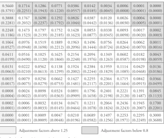
We estimated U by minimizing the relative entropy also over this parameter (see equation (14)). This resulted in an estimate of 0.764 for U. The corresponding transition matrix is displayed in Table 3 (values in parentheses). It is similar to the 3-band transition matrix but it shows less mobility as can be seen from Table 5. The chances to move out of low income classes as well as the chances to remain in the highest income class are higher.
Figure 4: Schrödinger Multipliers for the 3-Band-Hypothesis
1 2 3 4 5 6 7 8 9 10
0.6 0.7 0.8 0.9 1.1 1.2 1.3 1.4 1.5 1.6
1.0
I1989
Table 3: Hypothesized and Adjusted Transition Matrix for the AR(1) Model ( U 0.764) 0.5660 (0.3791) 0.1714 (0.2251) 0.1286 (0.1943) 0.0771 (0.1220) 0.0386 (0.0557) 0.0142 (0.0185) 0.0034 (0.0045) 0.0006 (0.0008) 0.0001 (0.0001) 0.0000 (0.0000) 0.3888 (0.2281) 0.1767 (0.2032) 0.1690 (0.2237) 0.1292 (0.1792) 0.0826 (0.1044) 0.0387 (0.0442) 0.0120 (0.0136) 0.0026 (0.0030) 0.0004 (0.0005) 0.0000 (0.0001) 0.2248 (0.1186) 0.1473 (0.1523) 0.1797 (0.2139) 0.1752 (0.2185) 0.1428 (0.1623) 0.0853 (0.0877) 0.0338 (0.0345) 0.0093 (0.0098) 0.0017 (0.0020) 0.0002 (0.0003) 0.1064 (0.0527) 0.0976 (0.0948) 0.1519 (0.1698) 0.1889 (0.2212) 0.1963 (0.2096) 0.1496 (0.1444) 0.0756 (0.0724) 0.0264 (0.0264) 0.0062 (0.0070) 0.0011 (0.0016) 0.0411 (0.0199) 0.0516 (0.0490) 0.1025 (0.1120) 0.1625 (0.1860) 0.2154 (0.2248) 0.2094 (0.1976) 0.1349 (0.1263) 0.0602 (0.0587) 0.0182 (0.0198) 0.0043 (0.0059) 0.0131 (0.0063) 0.0222 (0.0210) 0.0562 (0.0613) 0.1138 (0.1299) 0.1924 (0.2002) 0.2384 (0.2244) 0.1959 (0.1829) 0.1114 (0.1085) 0.0429 (0.0468) 0.0136 (0.0186) 0.0035 (0.0017) 0.0079 (0.0075) 0.0256 (0.0279) 0.0662 (0.0753) 0.1427 (0.1481) 0.2255 (0.2117) 0.2364 (0.2201) 0.1715 (0.1664) 0.0842 (0.0915) 0.0366 (0.0499) 0.0008 (0.0004) 0.0024 (0.0022) 0.0098 (0.0105) 0.0324 (0.0363) 0.0891 (0.0909) 0.1796 (0.1658) 0.2401 (0.2198) 0.2221 (0.2120) 0.1391 (0.1487) 0.0845 (0.1133) 0.0002 (0.0001) 0.0006 (0.0005) 0.0032 (0.0033) 0.0134 (0.0145) 0.0471 (0.0464) 0.1211 (0.1078) 0.2064 (0.1824) 0.2436 (0.2243) 0.1945 (0.2007) 0.1700 (0.2201) 0.0000 (0.0000) 0.0001 (0.0001) 0.0009 (0.0009) 0.0047 (0.0048) 0.0210 (0.0196) 0.0689 (0.0582) 0.1497 (0.1256) 0.2253 (0.1971) 0.2295 (0.2249) 0.3000 (0.3688)
Adjustment factors above 1.25 Adjustment factors below 0.8
hypothesized transition matrix in parenthesis
classes and in the highest classes has to be reduced. A look at Bartholomew’s index and the period mobility index shows that like in the 3-band hypothesis, equilibrium mobility is reduced and convergence mobility is increased as a result of the adjustment process.
Figure 5: Schrödinger Multipliers for the AR(1)-Hypothesis (U 0.764)
1 2 3 4 5 6 7 8 9 10
2.0
1.8
1.6
1.4
1.2
1.0
0.8
0.6
0.4
I1989
I1979
The three previously examined cases aimed at answering the question how to get information on the underlying process of income dynamics from cross-section information alone. The fourth example addresses a slightly different question: how to improve or update panel estimates of the income dynamics in the light of much more complete cross-section information. Somehow this seems to be the most natural application of our method. We take the estimated transition matrix from the PSID-panel as our starting point and seek for the most probable adjustment in the light of the larger and thus more complete information from the cross-section data used by Burkhauser et al. (1999).
19 Because our method shows the best result if there are no zero-entries in the hypothesized tran-sition matrices, we used 2-dimensional kernel density estimation to derive the PSID-model. out of 53,013. This type of data attrition is typical for panels over a long time span and demonstrates the usefulness of combining panel and cross-section infor-mation. We adjusted the PSID-data with the mean of the 1989 Burkhauser et al. data. Based on the reported incomes, we estimated a transition matrix defined on the same income classes as before.19 This matrix is labeled PSID model and reported in Table 4 (numbers in parentheses). The transition matrix estimated from the PSID data delivers a reasonable and perfectly valid specification. Unlike for the previous models, it is not possible to question a priori the PSID-model because it relies on actual data.
Table 4: Hypothesized and Adjusted Transition Matrix for the PSID Model
0.3753 (0.2817) 0.1513 (0.1655) 0.1160 (0.1407) 0.0953 (0.1221) 0.0868 (0.1018) 0.0630 (0.0690) 0.0503 (0.0534) 0.0443 (0.0469) 0.0160 (0.0170) 0.0018 (0.0018) 0.2769 (0.1987) 0.1427 (0.1492) 0.1539 (0.1785) 0.1316 (0.1610) 0.1051 (0.1178) 0.0765 (0.0801) 0.0564 (0.0573) 0.0381 (0.0385) 0.0149 (0.0151) 0.0039 (0.0038) 0.1812 (0.1248) 0.1183 (0.1188) 0.1629 (0.1814) 0.1626 (0.1910) 0.1534 (0.1651) 0.1106 (0.1112) 0.0576 (0.0562) 0.0286 (0.0278) 0.0145 (0.0142) 0.0103 (0.0096) 0.1265 (0.0859) 0.0897 (0.0888) 0.1318 (0.1446) 0.1597 (0.1849) 0.1841 (0.1953) 0.1571 (0.1558) 0.0891 (0.0856) 0.0371 (0.0355) 0.0155 (0.0150) 0.0095 (0.0087) 0.0833 (0.0563) 0.0580 (0.0572) 0.0980 (0.1071) 0.1379 (0.1590) 0.1872 (0.1977) 0.2083 (0.2056) 0.1418 (0.1358) 0.0595 (0.0567) 0.0206 (0.0197) 0.0055 (0.0050) 0.0477 (0.0322) 0.0355 (0.0350) 0.0676 (0.0738) 0.1132 (0.1304) 0.1825 (0.1927) 0.2338 (0.2307) 0.1808 (0.1730) 0.0942 (0.0898) 0.0346 (0.0331) 0.0102 (0.0093) 0.0349 (0.0239) 0.0190 (0.0190) 0.0382 (0.0423) 0.0795 (0.0930) 0.1406 (0.1506) 0.1949 (0.1951) 0.2075 (0.2014) 0.1634 (0.1579) 0.0838 (0.0815) 0.0381 (0.0353) 0.0266 (0.0185) 0.0086 (0.0087) 0.0179 (0.0202) 0.0490 (0.0582) 0.0878 (0.0955) 0.1461 (0.1485) 0.2236 (0.2204) 0.2238 (0.2196) 0.1430 (0.1411) 0.0735 (0.0691) 0.0223 (0.0157) 0.0042 (0.0043) 0.0094 (0.0107) 0.0356 (0.0425) 0.0667 (0.0731) 0.1332 (0.1364) 0.2140 (0.2125) 0.2235 (0.2210) 0.1695 (0.1686) 0.1217 (0.1153) 0.0029 (0.0020) 0.0012 (0.0013) 0.0087 (0.0100) 0.0288 (0.0348) 0.0535 (0.0592) 0.1101 (0.1139) 0.1131 (0.1135) 0.1349 (0.1347) 0.1603 (0.1610) 0.3865 (0.3697)
Adjustment factors above 1.25 Adjustment factors below 0.8
The Schrödinger multipliers in Figure 6 and the adjusted matrix reported in Table 4 indicate that the probabilities to stay in and to fall back to the lowest income class have to be increased considerably. Moreover, the probabilities to move up into higher income classes must be adjusted downwards for the low income classes. As for the previous specifications, the adjustment leads to a reduc-tion in Prais’ mobility index (see Table 5). Again, a look at the main diagonal shows that this decrease shows up because the rise in persistence in income classes 1 and 6 to 10 is larger than the rise in mobility in income classes 2 to 5. In con-trast to the 3-band and the AR(1) hypotheses, the adjustment results in a rise in both equilibrium and convergence mobility, as measured by Bartholomew’s index and the period mobility index, respectively.
Because the PSID-hypothesis is based on actual data (n 692 individuals), we can test for the appropriateness of this hypothesis. We treat the cross-sectional distributions m1979 and m1989 as known and equal to the true (population) dis-tribution. This is not an unrealistic assumption given the large sample size (see Table 1). The problem of adjusting the transition probabilities estimated from the PSID data can then be treated as the problem of estimating the cell proba-bilities of a contingency table for which the population marginal probaproba-bilities are known and fixed (Ireland and Kullback 1968; Aebi, Neusser, and Steiner
Figure 6: Schrödinger Multipliers for the PSID-Hypothesis
1 2 3 4 5 6 7 8 9 10
0.6 0.7 0.8 0.9 1.0 1.1 1.2 1.3 1.4
1999). In this case, the sample size n equals the number of observations from the PSID data, in our case 692. With this interpretation, the value of the test sta-tistic (21) becomes 11.51 (see Table 5) which does not lead to a rejection of the hypothesis that the PSID model is compatible with the cross-sectional observa-tions. Although the PSID model is not rejected, we still use the adjusted transi-tion matrix for further computatransi-tions because the adjusted matrix is at least as close to the true dynamics as the hypothesis.
As a final exercise we use the adjusted transition matrices to project the 1989 income distribution ten years into the future. The corresponding distributions in 1999, m1999, and the implied invariant distributions are reported in Table 6. For each distribution we also computed Atkinson’s inequality index, AH, and the generalized entropy index, GED. The maximum mobility transition matrix maps m1989 into itself so that the distribution is expected to remain unchanged.
Table 5: Summary Measures of the Four Hypotheses
maximal mobility
3-band-hypothesis
AR(1)-hypothesis
PSID-hypothesis Bartholomew’s mobility index a
hypothesized transition matrix 2.5957 1.5961 1.3835 1.6916 adjusted transition matrix 2.7750 1.5450 1.3317 1.7244 period mobility index b
hypothesized transition matrix 0.4904 0.0814 0.0363 0.2224 adjusted transition matrix 0.5246 0.0876 0.0380 0.2394 Prais’ mobility index c
hypothesized transition matrix 1 0.8694 0.8369 0.8683 adjusted transition matrix 1 0.8546 0.8313 0.8612
relative entropy 0.0077 0.0110 0.0203 0.0083
test statistic (distributed as F2
(9)) 11.51d
a Bartholomew’s index is defined as
§ §
iSi jp iij| j| where S is the invariant distributionof P.
b The period mobility index is the convergence index that corresponds to the equilibrium index given here by Bartholomew’s index (Aebi, Neusser, and Steiner 2006).
c Prais’ mobility index is defined as Ktr P( ) (K1).
The adjusted 3-band hypothesis implies a further increase in inequality. Note the increase of the size of the lowest three income classes as well as the increase in the top income class. In the long run, inequality is expected to increase even further although the size of the top income class shrinks below its 1989 level. This is due to the large increase of the size of the lowest income classes. Accord-ing to the adjusted 3-band hypothesis, we should see a large increase in the lower tail of the income distribution. The projections of the adjusted AR(1) model are quite similar to those of the adjusted 3-band hypothesis, both in the short and in the long run. The two hypotheses are remarkably similar concerning the direc-tion as well as the magnitude of the change. The adjusted PSID model produces similar results. Inequality is predicted to increase in the short as well as in the
Table 6: Projected and Steady State Distributions
Income class
observed distributions
projected distributions adjusted 3-band
model
adjusted AR(1) model
adjusted PSID model
m1979 m1989 m1999 SS m1999 SS m1999 SS
1 8.23 10.14 11.69 15.77 11.67 15.98 11.03 11.83
2 4.81 5.64 6.21 7.67 6.16 7.60 6.02 6.37
3 7.13 7.82 7.98 8.46 8.16 9.18 8.07 8.31
4 10.27 10.50 10.30 10.00 10.49 10.77 10.52 10.59 5 14.73 14.19 13.68 12.73 13.73 13.05 13.92 13.79 6 18.23 16.63 15.92 14.52 15.78 14.20 16.08 15.70 7 16.89 14.97 14.32 12.92 14.18 12.33 14.38 13.93
8 11.71 10.67 10.25 9.19 10.25 8.75 10.31 9.98
9 5.46 5.82 5.74 5.15 5.76 4.89 5.74 5.56
10 2.54 3.62 3.91 3.58 3.82 3.26 3.93 3.93
AH 0.5 0.0944 0.1080 0.1148 0.1271 0.1148 0.1266 0.1129 0.1160 GED 2 0.1993 0.2350 0.2522 0.2873 0.2526 0.2911 0.2483 0.2575
m1999 projected income distribution in 1999 based on the adjusted transition matrix with initial
income distribution m1989.
SS steady state or invariant distribution of the adjusted transition matrix. AH 0.5 Atkinson’s inequality index with H 0.5.
long-run. However, the raise in both inequality indices is considerably less pro-nounced. In contrast to the 3-band and the AR(1) hypothesis, the top income class is keeping its share in the long run.
4. Conclusion
This paper presents a method to estimate or adjust transition matrices using just cross-sectional observations at two points in time. The method has been applied to explain the development of the US income distribution, in particular the move-ment of the middle income classes. Irrespective of the prior specification, most of the mass corresponding to the middle income classes shifted downwards. These developments led to increased inequality which is expected to continue in the short as well as in the long-run. However, because we adjusted the 1979 data with the mean of the 1989 data to control for economic growth, our projections must be interpreted in relative terms. Therefore, our results do not contradict the pos-sibility that economic growth could “lift all boats”. But there is a clear tendency towards segregation in the US society.
Although the theory based models of income dynamics used in this paper are pretty simple, it is interesting to note that after applying our method to adjust the initial theory based models, the resulting projections point in the same direc-tion as the conclusions based on the empirically derived PSID-model. In order to make theory based models a serious alternative to empirical hypotheses, not just in qualitative but also in quantitative analysis, further investigations into theo-retic models of the underlying income dynamics are necessary.